
Singular Integral Neumann Boundary Conditions for Semilinear Elliptic PDEs


1
Department of Mathematics, Anand International College of Engineering, Jaipur 303012, Rajasthan, India
2
Nonlinear Dynamics Research Center (NDRC), Ajman University, Ajman AE 346, United Arab Emirates
3
Centre for Mathematics and Natural Sciences, Leipzig University of Applied Sciences, PF 30 11 66, 04251 Leipzig, Germany
*
Author to whom correspondence should be addressed.
Axioms 2021, 10(2), 74; https://0-doi-org.brum.beds.ac.uk/10.3390/axioms10020074
Submission received: 28 February 2021
/
Revised: 15 April 2021
/
Accepted: 21 April 2021
/
Published: 24 April 2021
(This article belongs to the Special Issue Special Functions Associated with Fractional Calculus)
Abstract
:In this article, we discuss semilinear elliptic partial differential equations with singular integral Neumann boundary conditions. Such boundary value problems occur in applications as mathematical models of nonlocal interaction between interior points and boundary points. Particularly, we are interested in the uniqueness of solutions to such problems. For the sublinear and subcritical case, we calculate, on the one hand, illustrative, rather explicit solutions in the one-dimensional case. On the other hand, we prove in the general case the existence and—via the strong solution of an integro-PDE with a kind of fractional divergence as a lower order term—uniqueness up to a constant.
1. Introduction
The aim of this article is to discuss (possibly singular) semilinear elliptic PDEs of the form
on bounded -domains subject to (possibly singular) integral Neumann boundary conditions
for a (possibly singular) kernel . Such integral boundary value problems occur in applications as mathematical models of nonlocal interaction between interior points and boundary points [1] and have been abstractly studied in the non-singular case by [2]. The linear case of Poisson’s problem and (non-integral) singular Neumann boundary conditions has been discussed in [3]; see [4] for the general linear case and [5] for nonlinear boundary conditions involving a measure. The existence of positive solutions to semilinear singular elliptic problems has been studied in [6] for homogeneous Dirichlet boundary conditions; for (non-integral) homogeneous Neumann boundary conditions, see [7]. For the semilinear problem (1) with (possibly singular) integral Neumann boundary condition (2), existence of very weak solutions , , with zero average has been shown in [8] under the assumptions on b that
- (A1)
- is a Carathéodory function; i.e., is measurable w.r.t. for every and continuous w.r.t. u for a.e. .
- (A2)
- b is bounded by with non-negative functions satisfying and for some , and ,
I.e., in the subcritical (w.r.t. ) and sublinear (w.r.t. u) case.
In this article, on the one hand, we discuss one-dimensional examples, which illustrate that without fixing the average the problem (1) and (2), has a one-dimensional continuum of solutions; on the other hand, we show that if the average is fixed, then problems (1) and (2), have a unique very weak solution under the additional assumption.
- (A3)
- is monotone w.r.t. u for a.e. with derivative bounded by a function satisfying ; particularly, we require .
2. Preliminaries
Let be a bounded domain. For an exponent , we denote the dual exponent by , and the Sobolev conjugate by for resp. Consider as arbitrary large for resp. Let for . Particularly, the dual of the Banach space of the p-integrable function u on can be identified with , the Sobolev embedding holds for , and the embedding is compact for due to the Rellich–Kondrachov theorem. Hereby, denotes the Sobolev space of functions u on having a p-integrable weak gradient , and functions in additionally satisfy Dirichlet boundary conditions on in the sense of traces [9]. Similarly, denotes the Sobolev space of functions u on having p-integrable second-order derivatives.
Let us exemplify the difference between strong, weak, and very weak solutions of linear elliptic partial differential equations (PDEs) by considering Poisson’s equation for a right hand side (r.h.s.) f. If , then is a p-integrable function; thus, for it makes sense to require almost everywhere (a.e.) in , and in this case, is called a strong solution Poisson’s equation. Correspondingly, , , is called the strong realization of the negative Laplacian.
However, if the r.h.s. is merely a distribution , then the existence of strong solutions cannot be guaranteed. However, weak solutions of Poisson’s equation subject to Dirichlet boundary conditions on may exist in the sense that
holds for every , and the operator defined on the left hand side (l.h.s.) is called the weak realization of the negative Dirichlet–Laplacian. Note that the l.h.s. arises from via partial integration using on . If the r.h.s. is an even worse distribution , then another partial integration leads to the notion of a very weak solution.
Definition 1.
A function is called a very weak solution of Poisson’s equation subject to Dirichlet boundary condition, if
is valid for every with on , and defined by letting be the l.h.s. of (4) is called the very weak realization of the negative Dirichlet–Laplacian.
Note that during partial integration the term arises, but as the derivative of v in direction of the outer normal vector along the boundary can be arbitrary, for functions f, validity of (4) ensures formally that u satisfies Dirichlet boundary conditions. Particularly, if , then holds with by Sobolev embeddings into Hölder spaces. Thus, if is a non-negative kernel not integrable over , but satisfying , then for the possibly non-integrable function on it still makes sense to consider very weak solutions of (4), where the definition of the r.h.s. makes sense due to
where for is used. This case is very similar to Brézis problem, where Poisson’s equation subject to Dirichlet boundary conditions on is considered for a measurable function satisfying . Brézis et al. [10] (see also [11]) have proved the existence and uniqueness of a very weak solution to this problem, and there is the notion of a very weak solution that prominently occurred for the first time. In this article, we are mainly interested in the very weak solution for the case of singular integral Neumann boundary conditions (instead of homogeneous Dirichlet boundary conditions) and semilinear (instead of linear) elliptic PDEs. To prove the existence and uniqueness, considering the above mentioned facts about Sobolev spaces, we used functional analytic methods like topological degree theory [12].
3. One-Dimensional Examples
In this section, we illustrate by one-dimensional examples—one example is linear but inhomogeneous; another one is sublinear but has vanishing r.h.s—that without fixing the average , the problem (1) and (2), has a one-dimensional continuum of solutions.
3.1. A Linear Example with Singular Right Hand Side
Example 1
(in [8]). In the one-dimensional case of the interval , where the boundary consists of two points, and for the kernel containing a parameter , , which is affine linear w.r.t. u and has a singularity of order as , Equation (1) reads as . In the special case , this is an inhomogeneous Cauchy–Euler ODE, and every solution has the form
Note that u does not admit a classical derivative at for parameters except for , or and . The integral Neumann boundary conditions (2) read in this example formally as and . In other words, the outflow through the boundary point 0 is given by the integral ; i.e., there is a nonlocal dependence of the outflow on a singularly weighted average of u over the domain, while there is no flow through the boundary point 1. Note that for every solution u of the form (5), the integral is infinite within the parameter range , except for , or and . Therefore, the integral Neumann boundary condition at the boundary point 0 reads formally as and thus is singular; i.e., there is an explosive inflow or outflow. Nonetheless, Equation (1) together with the singular integral Neumann boundary condition (2) at as well as the classical Neumann boundary condition at (corresponding to ) is satisfied for by the integrable functions for arbitrary in the very weak sense that
holds for every with . Thus, the very weak solutions of this singular integral boundary value problem form a one-dimensional affine linear subspace. Finally, fixing the average determines the constant C and hence the solution uniquely.
3.2. A Semilinear Example with Sublinear Kernel
Example 2.
Again, consider the one-dimensional case , now for the kernel with signed power , , which is sublinear for and has a singularity of order as . Then, Equation (1) reads as and is called an Emden–Fowler or Thomas–Fermi equation. As this equation is a second-order ODE, its general solution contains two constants. The boundary condition relates these constants by one equation. However, as the integral Neumann boundary condition is simply implied by integrating the ODE over Ω, it does not provide another equation for the constants. Hence, there is a one-dimensional continuum of solutions.
It remains to show that these solutions satisfy a singular Neumann BC at for and (and similarly for ). Elementarily, for implies due to that is positive near x; i.e., u is strictly convex near x. Hence, is strictly monotone increasing and, thus, due to negative for , so that is strictly monotone decreasing and positive for . In the weak formulation , put to obtain . As , we obtain , and, hence, tends to as due to Therefore, for and , every solution of on to the boundary value satisfies a singular Neumann boundary condition at .
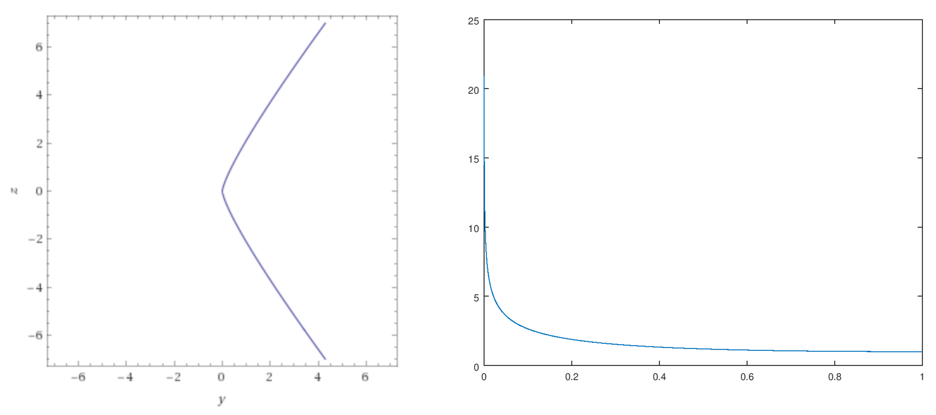
In the special case of , solutions can be more precisely described by , where solves the autonomous ODE and t is related to x by . This autonomous ODE can principally be solved by substituting , which leads to the first-order ODE . In the case , we obtain by separation of variables the equation with a constant . As holds, satisfies the implicit ODE . A phase plot of y is shown in the left of Figure 1 for , and a numerical solution u with and showing singularity at is plotted to the right in Figure 1.
4. Existence
In this section, for dimensions , let us briefly extend the proof of existence of very weak solutions from [8] to functions with an arbitrary pregiven average.
Theorem 1.
In the following, denote by
- D the subspacewhich has a compact embedding for .
- , the mixed fractional Sobolev space of order s and exponent q, which can be considered a space of functions v on such that is q-integrable over and is q-integrable over (particularly, ), where functions on are identified if they coincide a.e. on and a.e. on .
- ,the very weak realization of the negative Neumann–Laplacian .
- ,the realization of the nonlinearity and the integral Neumann boundary conditions, which may be singular.
Proof of Theorem 1.
Restrict A and B to the closed affine linear subspace of (of codimension 1) so that A becomes injective. By (A1) and (A2), is a bounded continuous mapping which becomes compact when viewed as mapping into due to the compactness of . Thus, we can view as a perturbation of A by a compact operator B. To conclude, regarding the existence of very weak solutions with , we may apply topological degree theory as in [8], but for this, we need to exclude the existence of solutions with an arbitrarily large -norm:
For with let be a strong solution of
subject to homogeneous Neumann boundary conditions on , where the constant is chosen such that the right hand side of (9) has zero integral. Thus, the compatibility condition is satisfied, and there exists a strong solution v of (9) subject to homogeneous Neumann boundary conditions, which is unique up to an additive constant. Moreover, such a solution v satisfies
with a constant independent of u, as holds by the definition of . Further, by the definition of v we have
due to and Jensen’s inequality . From (A2) we can conclude
with , and together with (10) both inequalities imply
As the right hand side tends to infinity for due to , the equation has no solution satisfying on the boundary of a sufficiently large ball around zero in . Therefore, like , also has a solution with . □
Remark 1.
Existence even holds in the linear case , , provided that or equivalently is sufficiently small.
5. Duality
To prepare the proof of uniqueness of very weak solutions to (1) and (2), let us consider in this section the affine linear case , where the sublinearity required in (A2) as well as the smallness condition mentioned in Remark 1 are not satisfied, but instead satisfies the same condition as in (A3); i.e., and and have average . Then problems (1) and (2) become linear and read (with w instead of u) as
The dual to this linear problem is
where , and
is a kind of fractional divergence of the function v with kernel .
Example 3.
Lemma 1.
Proof.
With the strong realization , , of the Neumann–Laplacian and the compact operator , we seek a solution of , i.e., a strong solution satisfying homogeneous Neumann boundary conditions. A problem closely related to (12) is
with . In fact, note that the weak formulation of this problem is the identification of a such that
for every . For with , the existence and uniqueness of the solution with follows Lax–Milgram and Poincáre inequality. In fact, the second term in (15) has the potential , and due to , the whole operator on the l.h.s. of the weak formulation has a coercive and weakly lower semicontinuous potential on .
Further, solving Poisson’s equation subject to inhomogeneous Neumann BC on , where is such that a (strong) solution exists. Then satisfies in with and on , i.e., (12), in a weak sense. Finally, due to and , the weak solution v is in fact a strong solution, and, by approximation, this also holds true under the regularity assumptions on in Lemma 1. □
6. Uniqueness
To prove the uniqueness of very weak solutions to (1) and (2), we additionally require b to satisfy (A3); i.e. the derivative is bounded by a function independent of u satisfying . As a consequence, the difference quotient is continuous w.r.t. for a.e. and thus a Carathéodory function.
Theorem 2.
Proof.
Let be two very weak solutions of (1) and (2), with identical averages . Let be a strong solution of
where
is a kind of fractional divergence of the function v with kernel , and is chosen such that there exists a solution v satisfying homogeneous Neumann boundary conditions on . Note that Lemma 1 guarantees the existence of such a strong solution. Now, test the difference between the equations solved by u and with the test function v to obtain
and due to , . Hence, holds. □
7. Conclusions
We were able to prove uniqueness up to a constant for very weak solutions to singular semilinear elliptic PDEs subject to singular integral Neumann boundary conditions. Our method to test for two very weak solutions of (1) and (2), with identical averages of the difference in the equations determined by the strong solution of a dual problem (which is an integro-PDE with a kind of fractional divergence as a lower-order term here), seems to be rather promising and may be applicable to show the uniqueness of very weak solutions for many other problems.
However, our results are still not optimal. For example, while we used an intermediate compact embedding , it seems to be an open question for which the direct embedding is compact. In fact, the embedding and interpolation properties of mixed fractional Sobolev spaces have not been studied in depth in the literature to date. Therefore, although there are some first steps, as in the Appendix B of [13], for example, how singular a domain-boundary kernel b can be without destroying the existence of solutions is an open question.
Author Contributions
Conceptualization, J.M. and P.A.; methodology, J.M.; software, G.S.; validation, J.M., P.A. and G.S.; formal analysis, J.M.; investigation, J.M.; resources, P.A.; data writing—original draft preparation, J.M.; writing—review and editing, J.M., P.A. and G.S.; visualization, G.S.; project administration, P.A.; funding acquisition, P.A. All authors have read and agreed to the published version of the manuscript.
Funding
This research was funded by the German DAAD/BMBF and the Indian DST for financial support within the DAAD-DST project PPP 2019 “Mathematical models of non-local interactions” grant number 57453186.
Acknowledgments
Jochen Merker is grateful to Jean-Michel Rakotoson, who suggested during the conference in Toulouse on the occasion of Peter Takáč’s birthday 2019 to prove uniqueness up to constants for solutions to semilinear elliptic PDEs with singular integral Neumann boundary conditions, and shared an idea of how to prove uniqueness under a kind of smallness condition.
Conflicts of Interest
The authors declare no conflict of interest.
References
- Avalishvili, G.; Avalishvili, M.; Gordeziani, D. On a nonlocal problem with integral boundary conditions for a multidimensional elliptic equation. Appl. Math. Lett. 2011, 24, 566–571. [Google Scholar] [CrossRef] [Green Version]
- Shakhmurov, V. Abstract elliptic equations with integral boundary conditons. Chin. Ann. Math. B 2016, 37, 625–642. [Google Scholar] [CrossRef]
- Merker, J.; Rakotoson, J.-M. Very weak solutions of Poisson’s equation with singular data under Neumann boundary conditions. Calc. Var. Partial. Differ. Equ. 2015, 52, 705–726. [Google Scholar] [CrossRef]
- Merker, J. On a generalization of Sobolev-Slobodecki spaces and an associated fractional derivative. In Proceedings of the International Conference on Fractional Differentiation and Its Applications (ICFDA), Amman, Jordan, 16–18 July 2018. [Google Scholar]
- Oussama Boukarabila, Y.; Véron, L. Nonlinear boundary value problems relative to harmonic functions. Nonl. Anal. 2015, 201, 112090. [Google Scholar] [CrossRef]
- Lair, A.; Shaker, A.W. Classical and Weak Solutions of a Singular Semilinear Elliptic Problem. J. Math. Anal. Appl. 1997, 211, 371–385. [Google Scholar] [CrossRef] [Green Version]
- Chabrowski, J. On the Neumann problem with singular and superlinear nonlinearities. Commun. Appl. Anal. 2009, 13, 327–340. [Google Scholar]
- Merker, J. Mixed fractional Sobolev spaces and elliptic PDEs with singular integral boundary data. Math. Meth. Appl. Sci. 2021, 44, 2859–2867. [Google Scholar] [CrossRef] [Green Version]
- Adams, R.A.; Fournier, J.J.F. Sobolev Spaces; Elsevier: Amsterdam, The Netherlands, 2003. [Google Scholar]
- Brézis, H.; Cazenave, T.; Martel, Y.; Ramiandrisoa, A. Blow-up for ut − Δu = g(u) revisited. Adv. Differ. Equ. 1996, 1, 73–90. [Google Scholar]
- Brézis, H.; Cabré, X. Some simple nonlinear PDE’s without solutions. Boll. Unione Mat. Ital. 1998, 1, 223–262. [Google Scholar]
- Cho, Y.; Chen, Y.Q. Topological Degree Theory and Applications; Chapman and Hall/CRC: New York, NY, USA, 2006. [Google Scholar]
- Merker, J. Very weak solutions of linear elliptic PDEs with singular data and irregular coefficients. Differ. Equ. Appl. 2018, 10, 3–20. [Google Scholar] [CrossRef]
Figure 1.
Left: phase portrait; right: solution curve.

Publisher’s Note: MDPI stays neutral with regard to jurisdictional claims in published maps and institutional affiliations. |
© 2021 by the authors. Licensee MDPI, Basel, Switzerland. This article is an open access article distributed under the terms and conditions of the Creative Commons Attribution (CC BY) license (https://creativecommons.org/licenses/by/4.0/).
Share and Cite
MDPI and ACS Style
Agarwal, P.; Merker, J.; Schuldt, G. Singular Integral Neumann Boundary Conditions for Semilinear Elliptic PDEs. Axioms 2021, 10, 74. https://0-doi-org.brum.beds.ac.uk/10.3390/axioms10020074
AMA Style
Agarwal P, Merker J, Schuldt G. Singular Integral Neumann Boundary Conditions for Semilinear Elliptic PDEs. Axioms. 2021; 10(2):74. https://0-doi-org.brum.beds.ac.uk/10.3390/axioms10020074
Chicago/Turabian StyleAgarwal, Praveen, Jochen Merker, and Gregor Schuldt. 2021. "Singular Integral Neumann Boundary Conditions for Semilinear Elliptic PDEs" Axioms 10, no. 2: 74. https://0-doi-org.brum.beds.ac.uk/10.3390/axioms10020074
Note that from the first issue of 2016, this journal uses article numbers instead of page numbers. See further details here.