
A Fractional-in-Time Prey–Predator Model with Hunting Cooperation: Qualitative Analysis, Stability and Numerical Approximations


Istituto per le Applicazioni del Calcolo “Mauro Picone” CNR, 80131 Napoli, Italy
*
Author to whom correspondence should be addressed.
Axioms 2021, 10(2), 78; https://0-doi-org.brum.beds.ac.uk/10.3390/axioms10020078
Submission received: 31 March 2021
/
Revised: 23 April 2021
/
Accepted: 27 April 2021
/
Published: 30 April 2021
(This article belongs to the Special Issue Differential Models, Numerical Simulations and Applications)
Abstract
:A prey–predator system with logistic growth of prey and hunting cooperation of predators is studied. The introduction of fractional time derivatives and the related persistent memory strongly characterize the model behavior, as many dynamical systems in the applied sciences are well described by such fractional-order models. Mathematical analysis and numerical simulations are performed to highlight the characteristics of the proposed model. The existence, uniqueness and boundedness of solutions is proved; the stability of the coexistence equilibrium and the occurrence of Hopf bifurcation is investigated. Some numerical approximations of the solution are finally considered; the obtained trajectories confirm the theoretical findings. It is observed that the fractional-order derivative has a stabilizing effect and can be useful to control the coexistence between species.
Keywords:
Caputo fractional derivative; Allee effect; existence and stability; Hopf bifurcation; implicit schemesMSC:
34A08; 34D20; 65R101. Introduction
Population dynamics are regulated by several factors: availability of resources, predation, diseases, etc. Among these factors, the interaction between prey and predators is probably the most studied one in ecology, tracing back to the works of Lotka and Volterra in the early 20th century. Since then, a number of predator–prey models have been proposed and studied (see the excellent reviews [1,2]), considering different extensions of the original one: the realistic assumption that prey populations are limited by food resources and not just by predation leads to the inclusion of terms representing carrying capacity for the prey population; the characterization of specific behaviors of the predator population results in the introduction of several functional responses for them; the complexity and dishomogeneity in the environment often requires a spatial description [3]. It is well-known that species diffusing at different rates can generate spatial patterns, observed in several biological contexts. Such Turing patterns affecting spatial predator–prey models have been deeply investigated in the literature. In addition, the inclusion of group defense has a significant impact on the dynamics of the predator–prey system. Of course, this movement is conditioned by the abundance or scarcity of the other species, so that spatio-temporal population models can include cross-diffusion terms in addition to self-diffusion ones.
Cooperation is a common behavior in many biological groups and can sensibly affect the growth rate of populations in an ecological community. Limiting our interest to the predator–prey dynamics, many mechanisms have been identified, all capable of facilitating reproduction, breeding, foraging and defense in the prey population. All of them can induce a demographic Allee effect [4]. In predators, hunting cooperation, among other interactions, can also result in Allee effects; different intensities of such a cooperative behavior impact on the survival of both species and modify the stability of the ecological system (see [5] and references therein).
Even if the interest on fractional calculus traces back at least to the 1970s (without considering the seminal suggestions given by Leibniz and Euler more than 300 years ago), in the last decades there has been an explosion of research activities on its application to several areas. Fractional order systems are not only an extension of conventional integer-order systems in mathematics but also have memory and hereditary properties that integer order systems do not have. In the last decades, there has been a huge interest in such models, due to their specific feature of describing memory effects in dynamical systems: many nonlinear models with time fractional derivatives have been considered, not only in population dynamics [6,7], but also in chemistry and biochemistry, medicine, mechanics, engineering, finance, psychology (see, among the recent surveys, [8,9]). In some situations, indeed, fractional-order models, enabling the description of the memory and hereditary properties inherent in various materials, processes and biological systems, seem more consistent with the real phenomena than integer-order models. Models with fractional-order derivatives can take different forms depending on the system considered; among them, fractional differential equations and fractional partial differential equations are greatly applied to describe continuous systems, both deterministic and stochastic [10]. In addition, heterogeneous non-ergodic diffusion processes [11] and the effect of anomalous diffusion on a population survival have been investigated [12].
The authors considered, in previous studies, some interacting population models that explored the mentioned characteristics (limited resources, nonlinear growth, fear effect, cooperative behavior), also in the presence of spatial dishomogeneity [13,14,15,16,17]. In the above-mentioned research, systems of both ordinary and partial differential equations have been studied. Precisely, ODE descriptions for the dynamics of an intraguild predator–prey model [13] and for the spreading of waterborne diseases [15,17] have been considered and the stability of the model solutions discussed. Furthermore, in order to highlight how the spatial diffusion can both play an important role in the population evolution and lead to the formation of spatial patterns, a reaction–diffusion system modeling hunting cooperation [14] and a predator–prey system with fear and group defense [16] have been analyzed. In such researches, the effect of spatial diffusion on the stability of the equilibria has been highlighted and the conditions on the parameters ensuring the formation of patterns (stripes, spots, mixed, etc.) have been found.
In the present paper, the authors generalize the model introduced in [5], by replacing the ordinary time derivative with a fractional one so to investigate how the fractional-in-time derivative impacts the system dynamics. It is worth underlining, for the sake of completeness, that such a model has been already extended in [14] to include spatio-temporal dynamics and the related occurrence of Turing patterns. Here, instead, the authors, to better highlight the fractional derivative impact on the populations dynamics, take into account the original ODE model and consider the corresponding fractional-in-time system.
Such a modeling provides challenges and ideas in many other fields of applied mathematics in which nonlinear mathematical models having a similar structure are considered [18,19,20,21,22]. After reviewing in Section 2 the main prerequisites on fractional calculus, the model is formulated in Section 3 and existence and boundedness of solutions is proved. Section 4 discusses the stability of the coexistence equilibrium, while Section 5 shows some numerical approximations by different schemes. Section 6 concludes the manuscript.
2. Preliminaries
In this section, we recall the fundamental definitions, concepts and results that we will use throughout the paper. For further details, we refer the reader to [23,24,25].
Definition 1.
The fractional integral of order for a Lebesgue integrable function is defined by
and the Caputo fractional derivative of order of a sufficiently differentiable function is defined by
where is the Euler’s Gamma function.
We underline that, under natural conditions on , the Caputo derivative coincides with the classical derivative whenever .
Lemma 1.
Let be a continuous function on satisfying , with and Then for it holds true
where is the Mittag–Leffler function defined by
Lemma 2.
Let , with , be the system with the initial condition and . If satisfies the Lipschitz condition with respect to x, then there exists a unique solution of the above system on
Lemma 3.
Let , with and be an autonomous nonlinear fractional-order system. A point is called an equilibrium point of the system if it satisfies This equilibrium point is locally asymptotically stable if all eigenvalues of the Jacobian matrix evaluated at satisfy the Matignon conditions
3. Fractional Model with Caputo Derivative: Statement of the Problem, Boundedness, Existence and Uniqueness
We present the following fractional-order prey–predator model corresponding to the non-dimensional model introduced in [5]
where represents the Caputo fractional derivative, given in Definition 1, with and are the non-dimensional variables corresponding to the prey and predator densities. All the non-dimensional parameters are positive constant. Precisely, k comprises the dimensional carrying capacity, the conversion efficiency as well as the per-capita predator mortality and attack rate, while is linked to the per-capita intrinsic growth rate of prey and per-capita mortality rate of predator and is linked to the predator cooperation in hunting rate, the attack rate and the per-capita predator mortality rate. Details on both the derivation of model and the biological meaning of parameters can be found in [5,14]. To (3) we append the initial conditions
3.1. Boundedness
In this subsection, we prove the positivity and boundedness of the solution of the system (3). Let and
Theorem 1.
Proof.
Let us define the function
and be a positive constant. Applying the Caputo fractional derivative on both sides in (5) and using (3), it follows that
where . Using Lemma 1, it follows that
Then, for it follows that Hence, all the solutions to (3) starting from are confined in the following domain
which is positively invariant. □
3.2. Existence and Uniqueness
In this subsection, we find the conditions for the existence and uniqueness of the solution to fractional-order prey–predator model (3) in the region , where
by using the fixed point technique. The existence of K is guaranteed by the boundedness of the solution. The model can be reformulated in the fractional integral form which gives
Denoting by and the following kernels
the following theorem holds.
Theorem 2.
Let and . If then the kernels agree with the contraction and Lipschitz conditions in the region
Proof.
Let and be two functions for the kernel and and be two functions for the kernel Then we have
and
where and Therefore, the Lipschitz conditions are satisfied for kernels and , and if then and are also contractions for and , respectively. Assume that the conditions (9) and (10) hold and let us consider the kernels and Then (7) can be written
The successive difference between the terms is defined as
where
□
The following theorem holds.
Theorem 3.
Proof.
This shows the existence for the solutions. Moreover, in order to prove that (18) are solutions to (3) and (4), we consider
where are the remaining terms. We show that the terms in (19) satisfy and Now, we consider the conditions
On using recursive techniques, we get
For , it follows that . In a similar way, we conclude that
In order to prove the uniqueness of the solution to the model (3) and (4), let us suppose there exists another solution of the system and . Then
In view of the Lipschitz condition, it follows that
and hence
In view of (17), it follows that and □
4. Stability Analysis
The equilibrium points of system (3) are obtained by considering
According to [5,14], besides the trivial equilibrium the system admits the predator-free equilibrium and the coexistence equilibrium where satisfies . As shown in [14], if is unique, while if and there exist two coexistence equilibria. In all other cases, no coexistence equilibria are admissible.
In the following, we will discuss the stability properties of the coexistence equilibrium by using the linearization method.
The Jacobian matrix of system (3) evaluated at the equilibrium point is given by
Now, the characteristic equation of the Jacobian matrix is and the roots of the characteristic equation are
where I and A are the trace and determinant of the Jacobian matrix given by
The stability analysis of will be divided in the following four cases:
- (1)
- If and , then are negative real numbers. Hence, The coexistence equilibrium is asymptotically stable.
- (2)
- If and then at least one of will be positive. Therefore, at least one of will be such that and hence the coexistence point is unstable.
- (3)
- When , then the eigenvalues are a pair of complex conjugate
- (a)
- If then and Then, when , the coexistence equilibrium is asymptotically stable, otherwise it is unstable.
- (b)
- If , then Then, and the equilibrium is asymptotically stable.
- (4)
- When and , then Hence, In this case, the equilibrium is asymptotically stable.
A Hopf bifurcation occurs when a pair of complex eigenvalues of the Jacobian matrix at an equilibrium point exists and the stability of the equilibrium changes from stable to unstable when a bifurcation parameter crosses a critical value. We can choose the order of derivation to be the bifurcation parameter and by using the following well-known result we find the conditions for the Hopf bifurcation to appear.
Lemma 4.
- the corresponding characteristic equation of system (3) has a pair of complex conjugate roots with
We find the conditions for the model (3) tp undergo a Hopf bifurcation at equilibrium point when the order of derivation passes through the critical value
Let us assume that and let the critical value Let us define and Then, it follows that the eigenvalues are a pair of complex conjugate with In addition, let then, it follows that
Finally,
Therefore, we can conclude that a Hopf bifurcation of (3) will appear at
5. Numerical Solution
Even if the interest on fractional calculus traces back at least to the 1970s (without considering the seminal suggestions given by Leibniz and Euler more than 300 years ago), in the last decades there has been an explosion of research activities on its application to several areas. Such a growing interest for fractional-order models had led to the development of specific algorithms devoted to the numerical approximation of the solution to fractional-order differential problems. Several solvers have been proposed in the last years [27,28,29], all trying to balance efficiency and accuracy while guaranteeing reliability of the numerical approximation. It is well-known, indeed, that the persistent memory of fractional-order operators reflects on the numerical evaluation of the solution: as a natural consequence, at each new timestep all the past history of the solution is to be considered. The number of involved steps increases with time, and so does the computational burden.
In a sense, numerical methods for fractional-order differential systems are then naturally multi-step. They generalize some of the ODE methods, but with significant differences in both complexity and accuracy. We follow here the excellent survey [30] and consider some of the schemes reported there. The simplest schemes are derived by approximating the integrand function in (7) by a piecewise polynomial and proceeding to its exact integration. This leads to “rectangular” (explicit or implicit) product integration formulas when a zero-order approximation of the integrand function in each subinterval is assumed, or “trapezoidal” formulas where first-order approximation is chosen. Of course, implicit formulas are more stable, but they require solving the nonlinear equations that generally arise. To avoid this additional burden, a predictor–corrector approach can be useful.
The convergence order of the rectangular formulas is one: the distance between the numerical approximation and the exact solution in any time point decreases linearly with the timestep, and this result replicates the well-known one for the ODE formula. Unfortunately, this is not always true for the trapezoidal rule: its convergence order is limited by the minimum between and 2 [28], so that for the rate of the corresponding ODE method cannot be reached. Similarly, higher order formulas for fractional systems do not lead to significant improvements in accuracy and convergence rate, and they are not worthy to be considered. As an alternative to product integration formulas, Fractional Linear Multistep methods have been proposed to generalize the standard multistep methods for ODEs. They are very robust and can reach higher convergence order, but their convolution weights are not known explicitly in advance and have to be evaluated. This computation can however be performed very efficiently by FFT derived algorithms.
Numerical approximations of the solution of (3) can then be obtained by applying several different schemes. Even developed from the same ODE methods, they present distinguishing characteristics that deserve to be investigated. For this reason, we considered and compared the following schemes:
- Implicit Rectangular Product Integration rule (PI1)
- Implicit Trapezoidal Product Integration rule (PI2)with = 1 and
- Predictor–Corrector Product Integration rule (PI12)
- Fractional Backward Differentiation Formula (FLMM2)
All these numerical schemes have been implemented in Matlab routines as given in [30,31]. For the problem at hand, the performance of these schemes can be evaluated only qualitatively, due to the lack of an exact (closed form) solution, by comparing their behavior for decreasing timesteps; however, we refer the reader to the above cited literature for an exhaustive assessment of their results on several test cases.
5.1. Preliminary Assessment
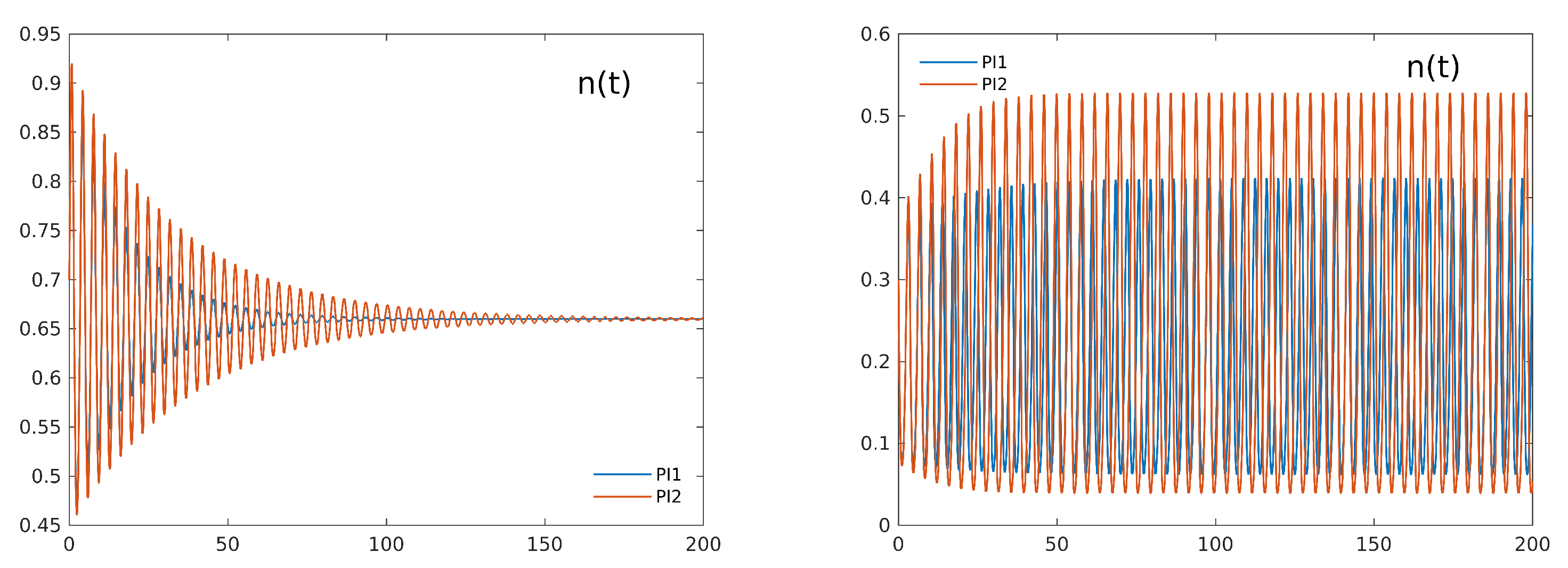
As a preliminary test, we checked the results of all methods in reproducing trajectories when = 1, because these results can be directly compared with the reference solutions given by classical ODE solvers. Even if the considered methods are all devised for fractional-order systems, they are expected to reproduce a good numerical approximation of the solution also for the integer order case. When the parameter settings ( = 3, = 0.3, k = 5) lead to a stable coexistence equilibrium, all methods are able to reproduce the expected trajectories: the left panel of Figure 1 shows the convergence of all numerical approximations of towards the equilibrium value 0.66. On the other hand, when Hopf instability occurs ( = 3, = 10, k = 0.8), the simplest PI1 method shows a sensible damping of the oscillations around the equilibrium 0.188, as shown in the right panel of the same Figure, while the other methods’ trajectories are practically indistinguishable from the reference one (as reported in [14]).
5.2. Stabilizing Effect of the Persistent Memory
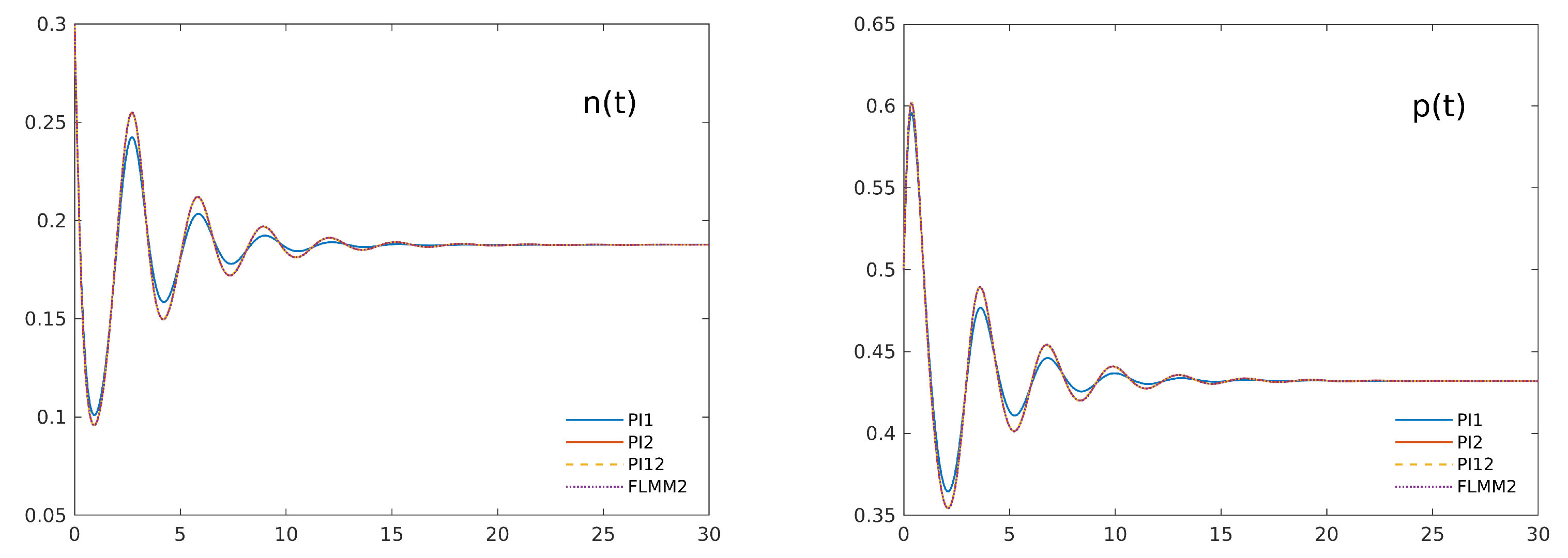
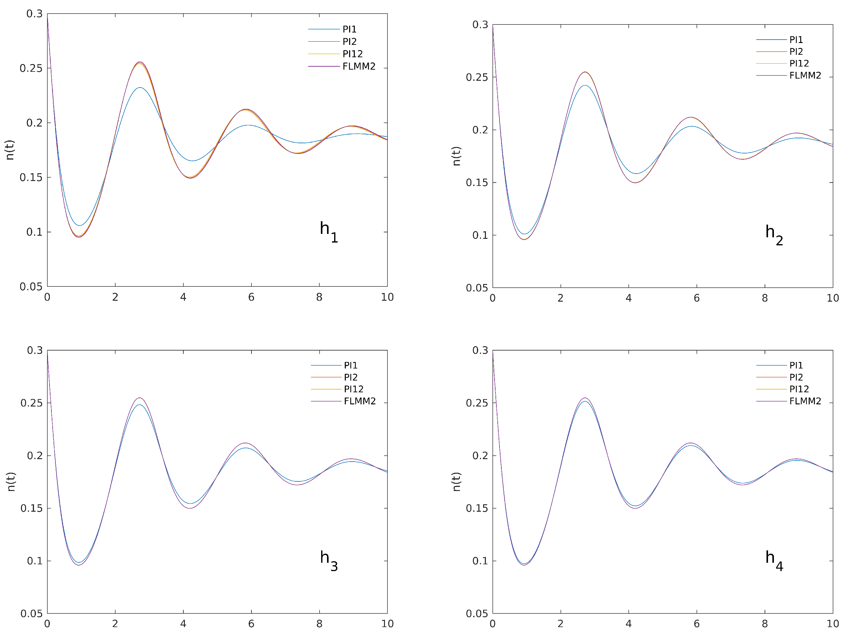
As a second test case, we consider a parameter setting for which the corresponding ODE system shows instability: if we choose as before = 3, = 10, k = 0.8, simply considering a slightly lower value for ( = 0.9) has a powerful stabilizing effect. As Figure 2 shows, all the numerical approximations agree in a fast damping of the oscillations for both the variables. Again, the damping is more evident in the lower order method PI1, while the other considered schemes agree in accurately reconstructing the system trajectories. To further analyze the different performance of the considered numerical methods, we present in the following Figure 3 a detail of the first part of the same trajectories as reconstructed by any of the numerical schemes for decreasing time steps . The less accurate results of PI1 with respect to the other schemes can be clearly seen. Of course, lower values for the fractional-order result in an even faster damping of the oscillations in the trajectories, confirming the strong stabilizing effect of the persistent memory in the model. For the same test case, Figure 4 compares the numerical approximations by PI2 of the populations’ trajectories for different values of the order (0.95, 0.9, 0.85, 0.8), confirming the strong stabilizing effect of the fractional derivative.
5.3. Hopf Instability for the Fractional System
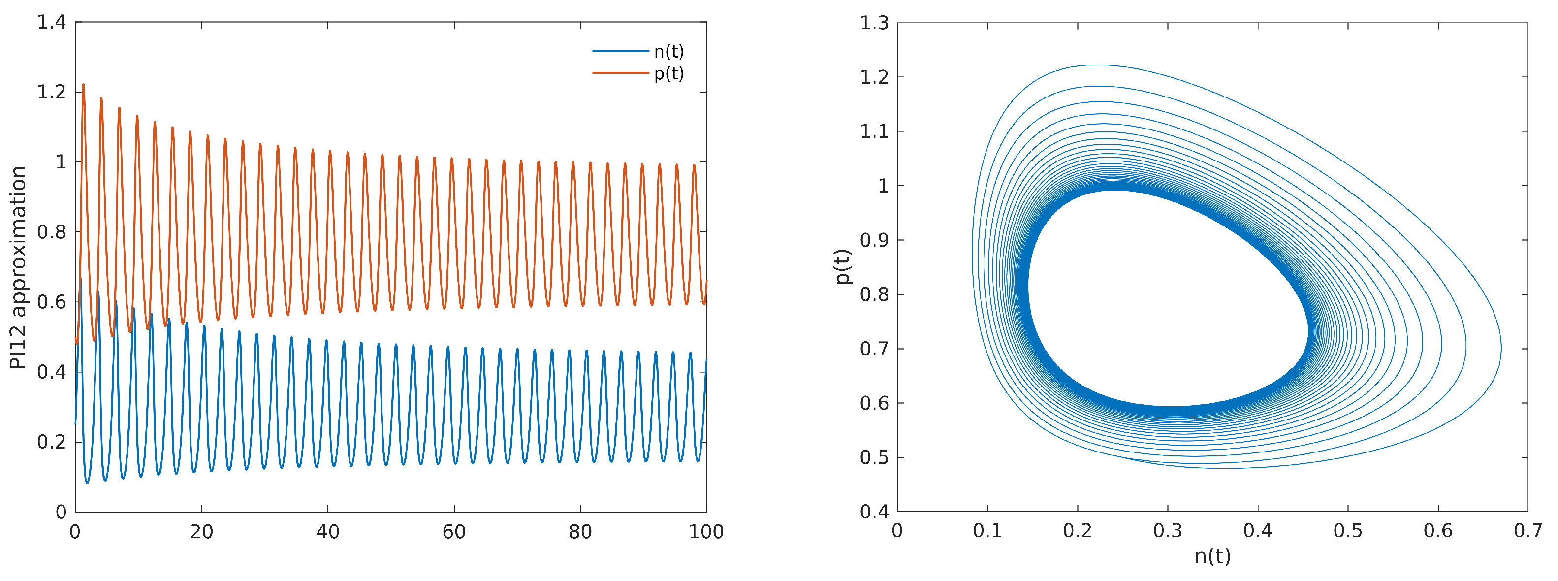
As a third example, we show how the instability can still occur for the fractional system with a suitable choice of the parameters. We start by considering a parameter setting for which, as stated in Section 4, the conditions for the Hopf instability to appear are met: we set = 3, = 3.5, k = 5. In this case, it is 0 and 0. The eigenvalues of the Jacobian are a couple of complex conjugate numbers with a positive real part so that for the coexistence equilibrium loses its stability. The following Figure 5 shows the trajectories of when = 0.92 as reconstructed by the more accurate numerical algorithms and the corresponding phase plan portrait, clearly showing the appearance of a limit cycle.
6. Conclusions
Fractional calculus, implying non-locality and memory effects, allows the description of numerous phenomena in a wide variety of scientific domains. Fractional-order operators have been proved to be a very powerful modeling instrument to represent a variety of processes and biological systems. In this framework, we studied in this paper the dynamic behavior of a fractional-in-time prey–predator model with hunting cooperation. The existence and uniqueness of a non-negative solution has been proved and the local stability of the coexistence equilibrium point has been analyzed by using the linearization technique. The conditions for the occurrence of a Hopf bifurcation have been found. Finally, numerical simulations have been presented to confirm by some selected examples how the order of derivation affects the dynamical behavior of prey and predator density. The findings of the present study, in our opinion, can provide hints for the investigation of the dynamics of other processes describing real-world phenomena. As a final consideration, we outline that several authors investigated pattern formation in the related spatial fractional-order systems. Recently, Yin and Wen [32] have shown that fractional-derivative systems can result in persistent spatial patterns even though their ODE counterpart does not induce any steady pattern. Such mechanisms of pattern formation along with the ones induced by anomalous diffusion suggest further directions of research in spatial generalizations of the considered model.
Author Contributions
Conceptualization, M.F.C. and I.T.; formal analysis, I.T.; numerical simulations, M.F.C.; writing (original draft preparation, review and editing), M.F.C. and I.T.; funding acquisition, M.F.C. and I.T. All authors have read and agreed to the published version of the manuscript.
Funding
This research was partially supported by Regione Campania Projects REMIAM, ADVISE and MEDIA.
Acknowledgments
This paper has been performed under the auspices of the G.N.F.M. and G.N.C.S. of INdAM.
Conflicts of Interest
The authors declare no conflict of interest.
References
- Abrams, P.A. The Evolution of Predator-Prey Interactions: Theory and Evidence. Annu. Rev. Ecol. Syst. 2000, 31, 79–105. [Google Scholar] [CrossRef]
- Berryman, A.A. The Origins and Evolution of Predator-Prey Theory. Ecology 1992, 73, 1530–1535. [Google Scholar] [CrossRef] [Green Version]
- Briggs, C.J.; Hoopes, M.F. Stabilizing effects in spatial parasitoid–host and predator–prey models: A review. Theor. Popul. Biol. 2004, 65, 299–315. [Google Scholar] [CrossRef] [PubMed]
- Courchamp, F.; Berec, L.; Gascoigne, J. Allee Effects in Ecology and Conservation; Oxford University Press: Oxford, UK, 2008. [Google Scholar] [CrossRef]
- Alves, M.T.; Hilker, F. Hunting cooperation and Allee effects in predators. J. Theor. Biol. 2017, 419, 13–22. [Google Scholar] [CrossRef]
- Tang, B. Dynamics for a fractional-order predator-prey model with group defense. Sci. Rep. 2020, 10, 4906. [Google Scholar] [CrossRef]
- Amirian, M.M.; Towers, I.; Jovanoski, Z.; Irwin, A.J. Memory and mutualism in species sustainability: A time-fractional Lotka-Volterra model with harvesting. Heliyon 2020, 6, e04816. [Google Scholar] [CrossRef]
- Patnaik, S.; Hollkamp, J.P.; Semperlotti, F. Applications of variable-order fractional operators: A review. Proc. R. Soc. Math. Phys. Eng. Sci. 2020, 476, 20190498. [Google Scholar] [CrossRef] [PubMed] [Green Version]
- Sun, H.; Zhang, Y.; Baleanu, D.; Chen, W.; Chen, Y. A new collection of real world applications of fractional calculus in science and engineering. Commun. Nonlinear Sci. Numer. Simul. 2018, 64, 213–231. [Google Scholar] [CrossRef]
- Abundo, M.; Ascione, G.; Carfora, M.F.; Pirozzi, E. A fractional PDE for first passage time of time-changed Brownian motion and its numerical solution. Appl. Numer. Math. 2020, 155, 103–118. [Google Scholar] [CrossRef]
- Cherstvy, A.G.; Chechkin, A.V.; Metzler, R. Ageing and confinement in non-ergodic heterogeneous diffusion processes. J. Phys. Math. Theor. 2014, 47, 485002. [Google Scholar] [CrossRef]
- Wang, W.; Cherstvy, A.G.; Liu, X.; Metzler, R. Anomalous diffusion and nonergodicity for heterogeneous diffusion processes with fractional Gaussian noise. Phys. Rev. E 2020, 102, 012146. [Google Scholar] [CrossRef]
- Capone, F.; Carfora, M.F.; De Luca, R.; Torcicollo, I. On the dynamics of an intraguild predator–prey model. Math. Comput. Simul. 2018, 149, 17–31. [Google Scholar] [CrossRef]
- Capone, F.; Carfora, M.F.; De Luca, R.; Torcicollo, I. Turing patterns in a reaction-diffusion system modeling hunting cooperation. Math. Comput. Simul. 2019, 165, 172–180. [Google Scholar] [CrossRef]
- Capone, F.; Carfora, M.F.; De Luca, R.; Torcicollo, I. Analysis of a model for waterborne diseases with Allee effect on bacteria. Nonlinear Anal. Model. Control 2020, 25, 1035–1058. [Google Scholar] [CrossRef]
- Carfora, M.F.; Torcicollo, I. Cross-diffusion-driven instability in a predator-prey system with fear and group defense. Mathematics 2020, 8, 1244. [Google Scholar] [CrossRef]
- Carfora, M.F.; Torcicollo, I. Identification of epidemiological models: The case study of Yemen cholera outbreak. Appl. Anal. 2020. [Google Scholar] [CrossRef]
- Torcicollo, I. On the nonlinear stability of a continuous duopoly model with constant conjectural variation. Int. J. Non-Linear Mech. 2016, 81, 268–273. [Google Scholar] [CrossRef] [Green Version]
- Rionero, S.; Torcicollo, I. On the dynamics of a nonlinear reaction-diffusion duopoly model. Int. J. Non-Linear Mech. 2018, 99, 105–111. [Google Scholar] [CrossRef]
- Rionero, S.; Torcicollo, I. Stability of a Continuous Reaction-Diffusion Cournot-Kopel Duopoly Game Model. Acta Appl. Math. 2014, 132, 505–513. [Google Scholar] [CrossRef] [Green Version]
- De Angelis, F.; De Angelis, M. On solutions to a FitzHugh-Rinzel type model. Ric. Mat. 2020. [Google Scholar] [CrossRef] [Green Version]
- Capone, F.; De Luca, R.; Rionero, S. On the stability of non-autonomous perturbed Lotka-Volterra models. Appl. Math. Comput. 2013, 219, 6868–6881. [Google Scholar] [CrossRef]
- Podlubny, I. Fractional Differential Equations. An Introduction to Fractional Derivatives, Fractional Differential Equations, Some Methods of Their Solution and Some of Their Applications; Academic Press: San Diego, CA, USA; London, UK, 1999. [Google Scholar]
- Diethelm, K. The Analysis of Fractional Differential Equations: An Application-Oriented Exposition Using Differential Operators of Caputo Type; Springer: Berlin/Heidelberg, Germany, 2010. [Google Scholar] [CrossRef] [Green Version]
- Kilbas, A.A.; Srivastava, H.M.; Trujillo, J.J. Theory and Applications of Fractional Differential Equations, Volume 204 (North-Holland Mathematics Studies); Elsevier Science Inc.: Amsterdam, The Netherlands, 2006. [Google Scholar]
- Li, X.; Wu, R. Hopf bifurcation analysis of a new commensurate fractional-order hyperchaotic system. Nonlinear Dyn. 2014, 78, 279–288. [Google Scholar] [CrossRef]
- Diethelm, K.; Ford, N.J.; Freed, A.D.; Luchko, Y. Algorithms for the fractional calculus: A selection of numerical methods. Comput. Methods Appl. Mech. Eng. 2005, 194, 743–773. [Google Scholar] [CrossRef] [Green Version]
- Garrappa, R. Trapezoidal methods for fractional differential equations: Theoretical and computational aspects. Math. Comput. Simul. 2015, 110, 96–112. [Google Scholar] [CrossRef] [Green Version]
- Cai, M.; Li, C. Numerical Approaches to Fractional Integrals and Derivatives: A Review. Mathematics 2020, 8, 43. [Google Scholar] [CrossRef] [Green Version]
- Garrappa, R. Numerical Solution of Fractional Differential Equations: A Survey and a Software Tutorial. Mathematics 2018, 6, 16. [Google Scholar] [CrossRef] [Green Version]
- Garrappa, R. FLMM2. MATLAB Central File Exchange. 2021. Available online: https://www.mathworks.com/matlabcentral/fileexchange/47081-flmm2 (accessed on 26 March 2021).
- Yin, H.; Wen, X. Pattern Formation through Temporal Fractional Derivatives. Sci. Rep. 2018, 8, 5070. [Google Scholar] [CrossRef] [PubMed] [Green Version]
Figure 1.
Trajectories for the numerical approximations PI1 and PI2 of solution of system (3) for = 1 in case of a stable equilibrium (left panel) and in the presence of Hopf instability (right panel). The lowest order approximation PI1 clearly shows damped oscillations, while the trajectories of the higher order approximations are in excellent agreement with the ones obtained by classical ODE solvers.

Figure 2.
Trajectories for all the numerical approximations of the solutions of system (3) in case = 0.9. While the corresponding ODE systems show instability (see the right panel of Figure 1), the trajectories of the fractional system rapidly stabilizes for both variables ( shown in the left panel, in the right one). The lowest order approximation PI1 clearly shows more damped oscillations, while the higher order approximations are all in excellent agreement.

Figure 3.
Details of the initial part of the trajectories shown in the left panel of Figure 2 as reconstructed by all the numerical methods for decreasing timesteps . The lowest order approximation PI1 clearly shows more damped oscillations, and only for the smallest timestep it agrees with the other methods, whose results are practically identical.

Figure 4.
Trajectories for the numerical approximations PI2 of the solutions of system (3) for different values (0.95, 0.9, 0.85, 0.8) for both populations ( shown in the left panel, in the right one). The stabilizing effect of the fractional operators can be clearly seen.
Figure 4.
Trajectories for the numerical approximations PI2 of the solutions of system (3) for different values (0.95, 0.9, 0.85, 0.8) for both populations ( shown in the left panel, in the right one). The stabilizing effect of the fractional operators can be clearly seen.

Figure 5.
Numerical approximation PI12 of the solutions of system (3) confirming the Hopf instability predicted by the theory in case = 0.92 with = 3, = 3.5, k = 5. In the left panel, the trajectories for both variables are reported as functions of time; the right panel shows the limit cycle in the phase plan.

Publisher’s Note: MDPI stays neutral with regard to jurisdictional claims in published maps and institutional affiliations. |
© 2021 by the authors. Licensee MDPI, Basel, Switzerland. This article is an open access article distributed under the terms and conditions of the Creative Commons Attribution (CC BY) license (https://creativecommons.org/licenses/by/4.0/).
Share and Cite
MDPI and ACS Style
Carfora, M.F.; Torcicollo, I. A Fractional-in-Time Prey–Predator Model with Hunting Cooperation: Qualitative Analysis, Stability and Numerical Approximations. Axioms 2021, 10, 78. https://0-doi-org.brum.beds.ac.uk/10.3390/axioms10020078
AMA Style
Carfora MF, Torcicollo I. A Fractional-in-Time Prey–Predator Model with Hunting Cooperation: Qualitative Analysis, Stability and Numerical Approximations. Axioms. 2021; 10(2):78. https://0-doi-org.brum.beds.ac.uk/10.3390/axioms10020078
Chicago/Turabian StyleCarfora, Maria Francesca, and Isabella Torcicollo. 2021. "A Fractional-in-Time Prey–Predator Model with Hunting Cooperation: Qualitative Analysis, Stability and Numerical Approximations" Axioms 10, no. 2: 78. https://0-doi-org.brum.beds.ac.uk/10.3390/axioms10020078
Note that from the first issue of 2016, this journal uses article numbers instead of page numbers. See further details here.