
Multicriteria Evaluation of Deep Neural Networks for Semantic Segmentation of Mammographies


Instituto Politécnico Nacional-CITEDI, 1310 Instituto Politécnico Nacional Ave, Nueva Tijuana, Tijuana 22430, Baja California, Mexico
*
Author to whom correspondence should be addressed.
†
These authors contributed equally to this work.
Axioms 2021, 10(3), 180; https://0-doi-org.brum.beds.ac.uk/10.3390/axioms10030180
Submission received: 5 July 2021
/
Revised: 25 July 2021
/
Accepted: 3 August 2021
/
Published: 5 August 2021
(This article belongs to the Special Issue Various Deep Learning Algorithms in Computational Intelligence)
Abstract
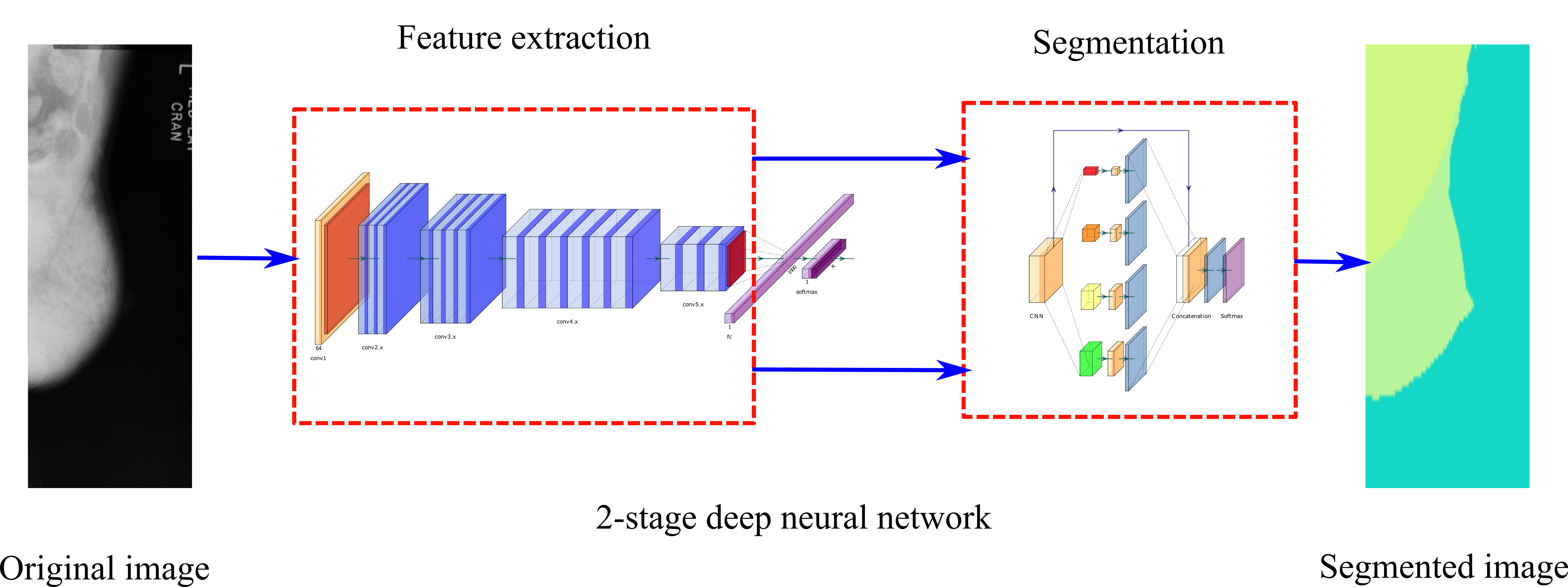
:Breast segmentation plays a vital role in the automatic analysis of mammograms. Accurate segmentation of the breast region increments the probability of a correct diagnostic and minimizes computational cost. Traditionally, model-based approaches dominated the landscape for breast segmentation, but recent studies seem to benefit from using robust deep learning models for this task. In this work, we present an extensive evaluation of deep learning architectures for semantic segmentation of mammograms, including segmentation metrics, memory requirements, and average inference time. We used several combinations of two-stage segmentation architectures composed of a feature extraction net (VGG16 and ResNet50) and a segmentation net (FCN-8, U-Net, and PSPNet). The training examples were taken from the mini Mammographic Image Analysis Society (MIAS) database. Experimental results using the mini-MIAS database show that the best net scored a Dice similarity coefficient of 99.37% for breast boundary segmentation and 95.45% for pectoral muscle segmentation.

1. Introduction
Computer-aided detection (CADe) systems are valuable tools to assist medical experts in detecting and diagnosing diseases. The aim of CADe for breast analysis is twofold: it reduces the chances of cancer being undetected in the earlier stages, and it can lower the number of unnecessary medical interventions (such as biopsies), mitigating the levels of anxiety and stress in the patients [1,2].
For mammogram CADe, accurate segmentation of the breast is a crucial step [3,4,5], as it can accelerate diagnosis and lower the number of false positives and false negatives [1,6,7]. Automatic mammogram segmentation identifies the different tissues in the breast and gives them a label such as pectoral muscle, fatty tissue, fibroglandular tissue, or nipple [6,7,8].
In breast segmentation, the most challenging task is to identify the pectoral muscle accurately. As a result, the brightness, position, and size of the pectoral muscle vary widely. The pectoral muscle may occupy most of the image or do not appear in it. Most of the time, the pectoral muscle appears in the upper part of the mammogram with a white triangular shape since the curvature and length of the lower edge fluctuates [7]. The pectoral muscle’s brightness can appear similar to fibroglandular tissue in dense breasts or other structures such as parenchymal texture, artifacts, and labels in digitized mammograms [6,9].
CADe approaches for image segmentation began with traditional computer vision techniques such as edge detection and mathematical modeling. These systems evolved and started including machine learning approaches which, at present, constitute the core of a CADe system, becoming the primary option for medical image segmentation [10]. Although deep learning has shown excellent performance for medical image segmentation, the use of deep learning for mammogram segmentation is scarce [4,11].
This paper contributes with an extensive evaluation of mammogram segmentation using deep learning architectures. We combined several architectures to explore their performance under different scenarios. We obtained accuracy metrics, memory consumption, and inference time to compare the performance of the architectures. We present multicriteria evaluation results that can help obtain answers beyond simple accuracy metrics since other important characteristics can also be considered in selecting the best architecture for a given application. Additionally, we provide a comprehensive introduction to the topic of semantic segmentation using deep learning approaches and how different deep neural networks can be combined to achieve better results.
The paper is organized as follows: in Section 2, we summarized the different state-of-the-art approaches for breast segmentation. In Section 3 the theoretical background of deep neural network used in this work and key concepts about digitized mammograms are provided. In Section 4 we provide information about the designed experiments and how to reproduce our findings. In Section 5, we present our results using the mini-MIAS database and a comparative against other methods. Finally, in Section 6 we discuss our results and provide our opinion about future work.
2. Related Work
Traditional methods for breast segmentation combine geometric models and iterative calculation of a threshold to distinguish between different breast tissues. Mustra and Grgic [5] used polar representation to identify the round part of the breast. They found the breast line using a combination of morphological thresholding and contrast limited adaptive histogram equalization. To extract the pectoral muscle, they used a mixture of thresholding and cubic polynomial fitting.
Liu et al. [8] developed a method for pectoral muscle segmentation based on statistical features using the Anderson–Darling test to identify the pectoral muscle’s boundary pixels. They eliminated the regions outside the pectoral muscle’s probable area by assuming the position of the pectoral muscle (upper-left corner of the mammogram) and found the final boundary of the muscle by using an iterative process that searches for edge continuity and orientation.
More recently, Taghanaki et al. [2] used a mixture of geometric rules and intensity thresholding to identify the breast region and the pectoral muscle. Vikhe and Thool [7] developed an intensity-based algorithm to segment the pectoral region. They estimated the pectoral region through a binary mask of the breast obtained by a thresholding technique followed by an intensity filter. Then, with a thresholding technique for rows separated by a pixel interval, several estimated pectoral muscle outline points were found.
Rampun et al. [3] developed a mammogram model to estimate the pectoral region’s position and the breast’s orientation. First, they found the breast region using Otsu’s thresholding, then removed the noise using an anisotropic diffusion filtering; after that, the initial breast boundary was found using the image’s median and standard deviation. The Chan–Vese model was used to obtain a more precise boundary. Finally, using an extended breast and Canny edge detection model, the pectoral muscle was found.
The use of deep learning in medical imaging has incremented since 2015 and is now an essential topic for research. In the medical field, deep learning has been used to detect, classify, enhance, and segmentation [12]. Despite this trend, the number of works published for mammograms with deep learning is low.
In this regard, Dalmış et al. [13] segmented breast MRI’s using several sets of U-nets. In the first experiment, they trained two U-nets, the first one for the breast area’s segmentation and the second one to segment the fibroglandular tissue. In the second experiment, a single U-net with three classes to identify the background, the fatty tissue, and the fibroglandular tissue was trained. They used the SØrensen–Dice similarity coefficient to evaluate the experiments, obtaining 0.811 for the first experiment and 0.85 for the second.
Dubrovina et al. [4], used a convolutional neural network (CNN) for pixel-wise classification of mammograms. In their work, they classify mammograms patches into five classes: pectoral muscle, fibroglandular tissue, nipple, breast tissue, and background.
In a recent work, de Oliveira et al. [11] used several semantic segmentation nets for mammogram segmentation. They used three different net architectures (FCNs, U-net, and SegNet) for the segmentation of the pectoral muscle, breast region, and background.
Rampun et al. [14] used a convolutional neural network for pectoral segmentation in mediolateral oblique mammograms. The network used by Rampun et al. was a modified holistically nested edge detection network. In a more recent work, Ahmed et al. [15] used two different architectures, Mask-RCNN and the DeepLab V3, for the semantic segmentation of cancerous regions in mammograms.
3. Theoretical Background
This section provides the mathematical foundation of the convolutional neural networks that we used to perform semantic segmentation of the breast; we explain key concepts about mammograms to facilitate the understanding of the methods, evaluation, and results. All the tested architectures of DNN are also explained.
3.1. Supervised Learning Foundations
The general problem in machine learning can be summarized as the following: given a collection of input values and a set of adjustable weights W, calculate an approximation function that estimates output values , see (1). The output can be seen as the recognized class label of the given pattern , as scores, or as probabilities associated with each class [16].
The loss function is calculated by Equation (2), where D measures the discrepancy between the desired valued and the output given by our approximation function F.
The average loss function, is the average of the errors over a set of labeled examples called the training set . A simple learning problem consists in finding the value W that minimizes . Commonly, the system’s performance is estimated by using a disjoint set of samples called the test set, [16].
A method to minimize the loss function, is by estimating the impact of small variations in the parameters W on the loss value. This is measured by the gradient of the loss function with respect W. Generally, W is a real-valued vector, in which is continues and differentiable [16]. The most simple minimization procedure is by using gradient descent, where W is adjusted in each step by:
where is called the learning rate, which indicates how much the algorithm would change by the calculated error.
Another popular minimization procedure is the stochastic gradient descent. This algorithm consists in updating the W using a noisy or approximated version of the average gradient. This can be represented as randomly selecting a subset of the input data and calculate an approximate gradient for each batch. Since over a set of iterations the addition of the loss functions would be calculated randomly for most of the data, the average of the different trials would be very similar to the real gradient. The stochastic gradient descent is represented as:
The main difference, is that in this case, is calculated over a subset of called x. In the most simple case, W is updated using only a single example. With this procedure, the calculated gradient fluctuates around an average trajectory that usually converges faster than the original gradient descent [16].
Feedforward networks use backpropagation to efficiently calculate gradients of differentiable layers. The basic feedforward networks is built as a group of cascade elements (neurons) each one implementing a function , where is the output of the module, is the vector of tunable parameters, and is the input of the module. The input to the first module is the input pattern X, and the subsequent layers that calculate are called hidden layers. If the partial derivative of with respect to is known, then the partial derivatives of with respect to and can be calculated using rule chain as:
where is the Jacobian of F with respect to W evaluated at the point , and is the Jacobian of F with respect to X. The full gradient is obtained by getting the average of the gradients over all the training patterns.
3.2. Convolutional Neural Networks
Multilayer networks can learn complex, high-dimensional, nonlinear mappings from a large set of training examples. This ability makes them a clear candidate for image recognition tasks. A typical pipeline of an image recognition system uses a feature extractor method to obtain the most relevant characteristics of the image and then use them as feature vectors to train the network. Most of these feature extractors are hand-crafted, which makes appealing the possibility of creating features extractors that learn the most relevant features. Using traditional neural networks (also called fully connected networks) for feature extraction and classification has some evident limitations.
The first one is the size of the network. Traditional images are multi-channel matrices with millions of pixels. To represent this information on a fully connected network, the number of weights for each fully connected layer would be in the millions even if the image is resized to a certain degree. The increment in the number of trainable parameters increases the memory requirements to represent the weights of the network.
Additionally, there is no built-in invariance of translation or local distortion of the inputs in these types of networks. In theory, a fully connected network could learn to generate outputs that are invariants to distortion or some degree of translation. The downside is that it would result that several learning units have to learn similar weight patterns that are positioned at different locations in the input. Covering the space of all the possible variations would need many training instances; hence it would demand considerable memory requirements.
Another deficiency of fully connected networks is that the topology of the input vector is ignored. Images have a solid two-dimensional local structure where pixels have a high correlation with their neighbors. These local correlations in images are the main reason for using hand-crafted feature extractors before a classification stage.
Convolutional neural networks (CNN) address the issues of fully connected networks and achieve shift, scale, and distortion invariance by using three elements: local receptive fields, shared weights, and spatial subsampling. Local receptive field neurons are used to extract elementary visual features such as edges, endpoints, corners, and textures. Subsequent layers combine these low-order features to detect higher-order features. On a CNN, learning units in a layer are organized in planes in which all units share the same set of weights, this allows the network to be invariant to shifts or distortions of the input. The set of outputs of the learning units is called a feature map [16]. The shared weights are adjusted during the learning phase to detect a set of relevant features.
A convolutional layer comprises several feature maps, this allows multiple features to be extracted at each location. The operation of the feature maps is equivalent to a convolution, followed by an additive bias and a squashing function, giving its name of convolutional network [17]. A convolutional layer can be represented as:
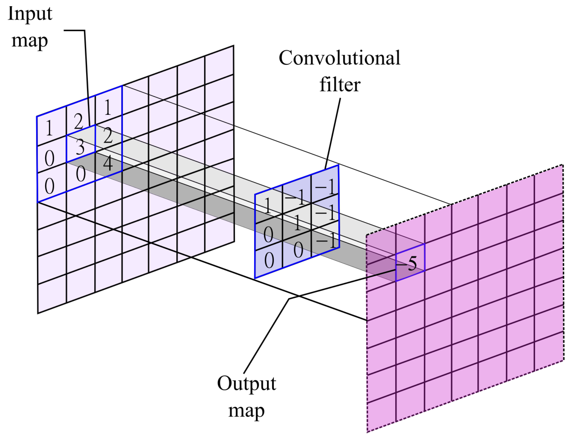
where K is the kernel that acts on the input map using a window of size k. The kernel of this convolutional layer is the set of connection weights used by the units in the feature map. In Figure 1, an arbitrary input map is feed into a convolutional filter with size . To obtain the output, each element in their respective position would be multiplied with their pairs in the input map at position and then they would be summed up. In this specific example, the operation is as follows: . The convolutional filter would move over the input map given a step size. The output map would be the encoded features from the input map given the convolutional filter.
The shape, size, and composition of the kernel helps the network to learn specific features that the network detects as important. Convolutional layers are robust to shift and distortions of the inputs since the feature maps only shifts by the same amount as the shift in the input image.
After a feature is detected, its exact position becomes irrelevant, and only the approximate position relative to other features is important. Knowing its precise position can be harmful to achieving robustness to slight variations of the input. In order to reduce precision, spatial resolution reduction of the feature maps is used in convolutional networks.
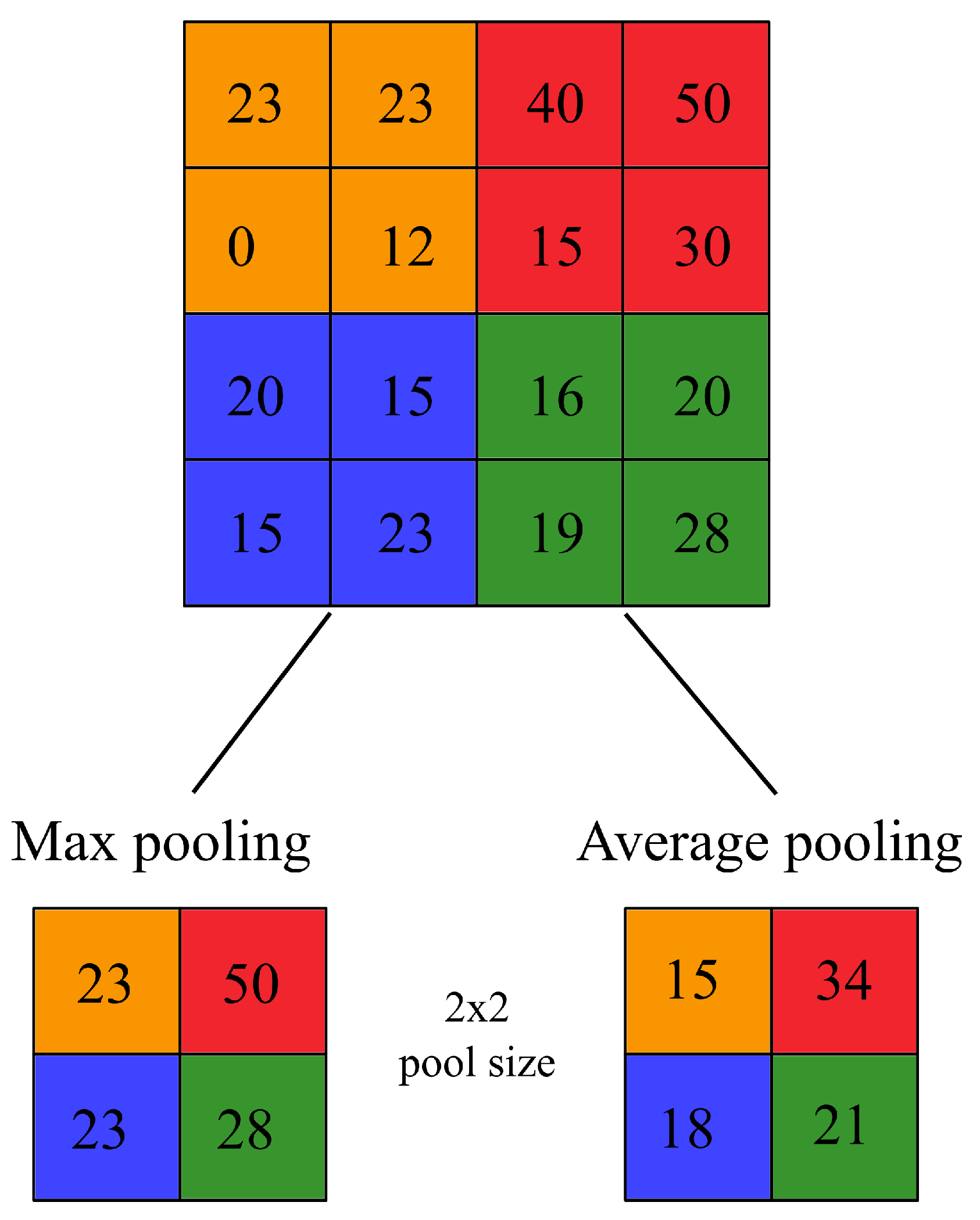
Pooling layers can perform a subsampling using a wide array of mathematical operations over a feature map. These operations can be as simple as the maximum value over a given window (max pooling), the average value (average pooling), or more complex, such as taking the average of the whole feature map (global average pooling). Similar to the convolutional layers, the mathematical operation of pooling layers acts upon a fixed window of size p. In Figure 2, two different pooling layers of size are applied over an given feature map of size . Given , the feature map is downsized to . The colors indicate the area of effect of the pooling layer. As an example, on the orange layer, the output of the max-pooling is 23 given that the maximum value is 23, on the contrary, for the average pooling (rounded to the next integer value) the output is 15 given that . Selecting over different pooling layers would affect the learning capacity of the network.
Using a combination of convolutional and pooling layers over a progressing reduction of spatial reduction compensated by an increasing number of feature maps helps achieve invariance to the geometric transformation of the input.
At the end of the convolutional and pooling layers, a fully connected network is used. Since all the weights in the system are learned using backpropagation, and at the end there is a fully connected network, in essence, a CNN is learning to extract its own features and classify them.
CNNs are an example of deep neural networks (DNNs), which are neural networks with many layers between the input layer and the output layer (hidden layers), hence the name.
3.3. Fully Convolutional Networks
Fully convolutional networks (FCN) are a particular type of CNNs, where all the layers compute a nonlinear filter (a convolutional filter). This allows FCNs to naturally operate on any input size and produce an output of the corresponding spatial dimensions [18].
Commonly, detection CNNs take fixed-sized inputs and produce nonspatial outputs. Fully connected layers can also be viewed as convolutions with kernels that cover the entire input. This can transform traditional CNN into FCNs that take input of any size and make spatial output maps.
These outputs maps are typically reduced due to the subsampling provided by the pooling layers, reducing the resolution of the FCNs by a factor equal to the pixel stride of the receptive fields of the output units; this is to prevent the coarse outputs from being connected with upsampling layers that act as convolutional layers with a fractional input stride of . These fractional stride convolutions are typically called transpose convolutions.
A network with these characteristics can perform classification at a pixel level or semantic segmentation. In semantic segmentation, every pixel of the image is associated with a class. This association helps to understand what is happening in the image and where it is happening [18].
3.4. Deep Learning Architectures for Semantic Segmentation
Many deep neural networks (DNNs) have been proposed for semantic segmentation, most of these approaches are based on a derivation of the following: convolutional neural networks, fully convolutional networks [18], U-Net [19] variations, convolutional residual networks, recurrent neural networks [10], densely connected convolutional networks [20], and DeepLab variations [21,22,23].
In this work, we used several DNNs to test their performance in mammogram segmentation. Similar to Siam et al. [24], we combined pairs of feature extraction networks and segmentation networks for semantic segmentation. For the feature extraction section, we used the VGG16 and the ResNet50; for the segmentation part, we used FCN8, U-Net, and PSPNnet. These composite structures summarize the spectrum of DNNs for semantic segmentation.
In the following lines, we describe the base networks used in this work in detail, followed by the description of the specific encoder–decoder pairs used for the breast segmentation.
3.4.1. VGG16
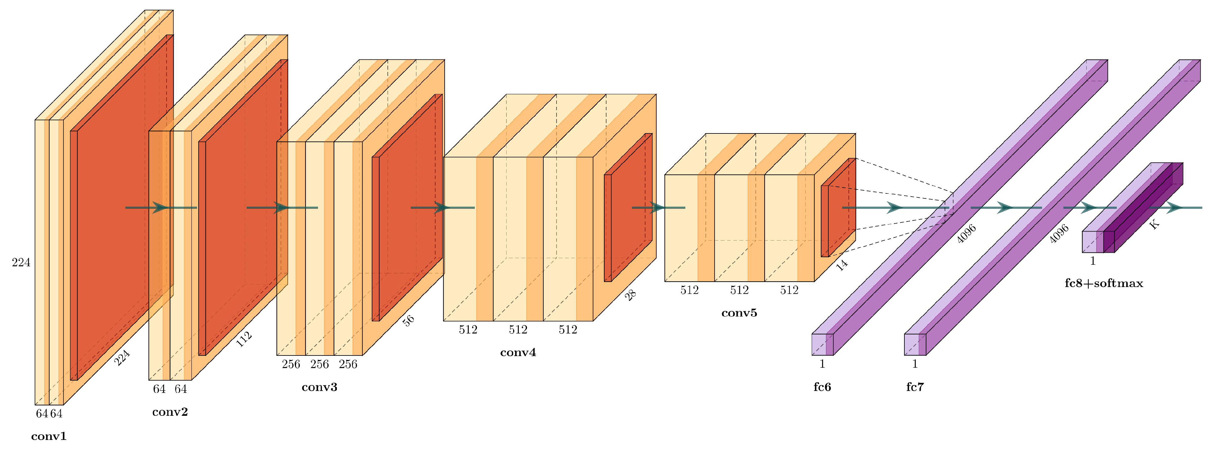
Simonyan and Zisserman [25] proposed VGG16, which is a well-known architecture that won the 2014 ImageNet Challenge. The VGG16 has 16 weight layers (convolutional and fully connected layers), with a total of 134 million trainable parameters, see Figure 3.
The input layer has a fixed size of , followed by five convolutional sections. Each convolutional section have filters with a stride of 1, followed by a max-pooling filter with stride 2. The activation function used in each block are rectified linear units (ReLU) layers, defined as:
The end layers are three fully connected layers: the first two with 4096 channels, and the third one is a softmax layer with the number of channels adjusted to the number of classes. Table 1 describes each layer in detail.
3.4.2. ResNet50
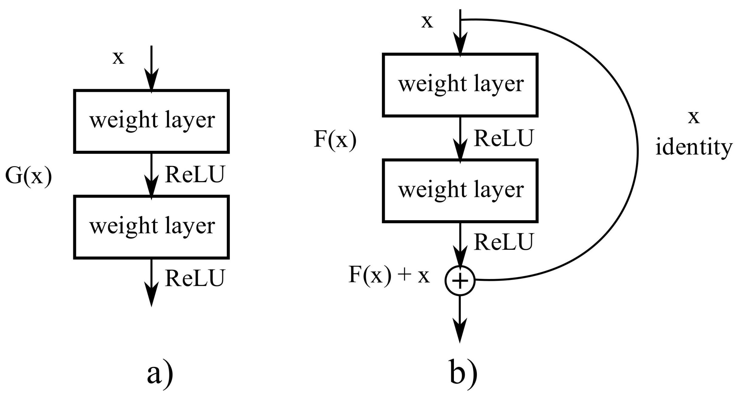
A big obstacle for earlier networks with depth above thirty layers was accuracy saturation, followed by a fast accuracy degradation. ResNet was proposed by He et al. [26], winning the ILSVRC classification task in 2015. ResNet addresses the degradation problem with residual blocks, see Figure 4, which are shortcut connections between layers using identity mapping, and adding their outputs of the stack layers.
ResNets have five sections: the first section is a convolutional layer followed by a max-pooling layer; the other four sections are residual blocks that repeat different times. ResNet50 is the fifty layer variant of ResNet, see Figure 5, their four residual blocks are called bottlenecks. Each bottleneck block has three convolutional layers, the first and the third one have kernels, and the second layers have a kernel. A description of the layers in ResNet50 can be found in Table 2.
3.4.3. FCN-8
Fully convolutional networks were one of the first networks designed for semantic segmentation [18]. Their main advantage was their capacity to take an input of arbitrary size, generating a correspondingly sized output.
The fully convolutional versions of classification networks (such as Alexnet, VGG16, GoogLeNet) add skip connections at the end of convolutional blocks, and they add a convolutional filter in the output and fuse it with an upsampled region at the end of the network. The upsampling layers are transposed convolutional layers.
In FCNs, fully convolutional layers replace the fully connected layers at the end of the classifiers: instead of having p neurons interconnected, the layer will have p convolutional layers. At the end of the network, a softmax layer classifies every pixel into a class.
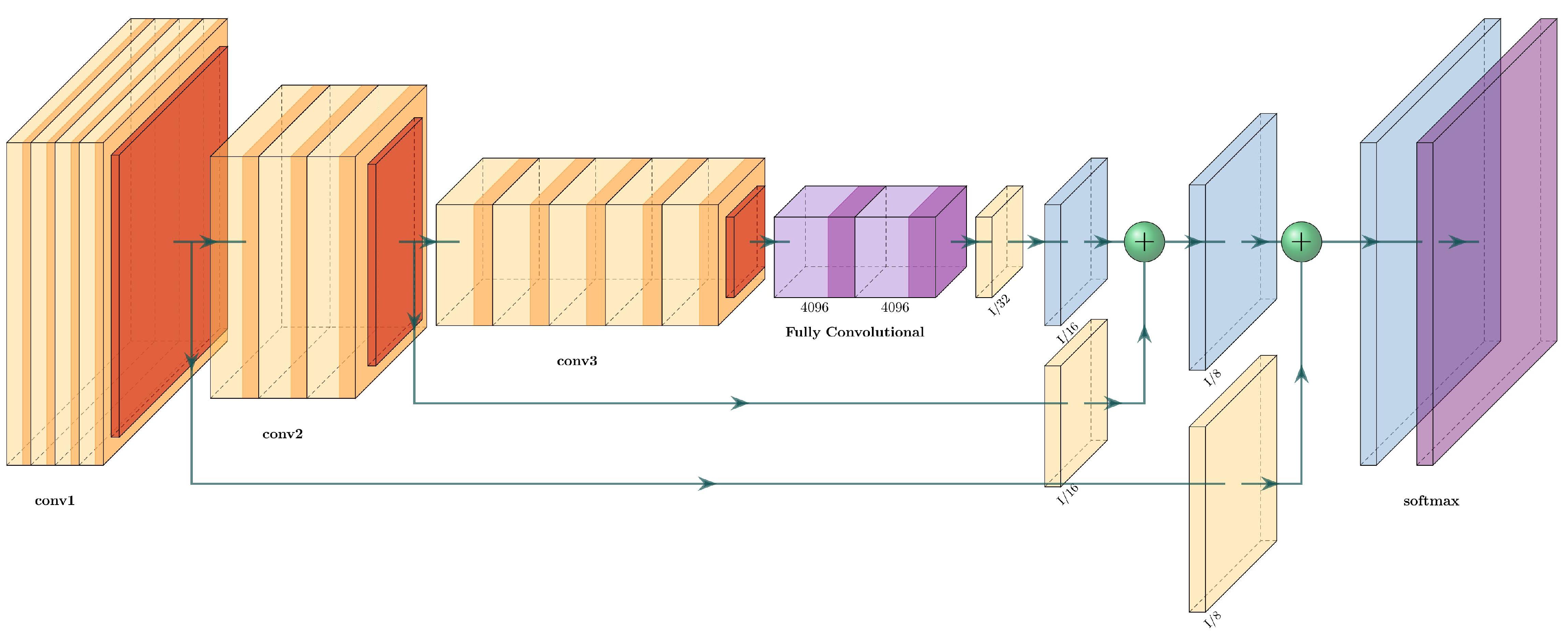
The FCN8 has two skip connections and three upsampling layers. The first upsampling layer feeds directly from the fully convolutional layers and has a stride of 32. The second and third upsampling layers are fed from the skip connections and have 16 and 8 strides, respectively. The two skip connections come from upper pooling layers, and each one passes through a convolutional layer. An example of an FCN-8 for an arbitrary network is shown in Figure 6.
3.4.4. U-Net
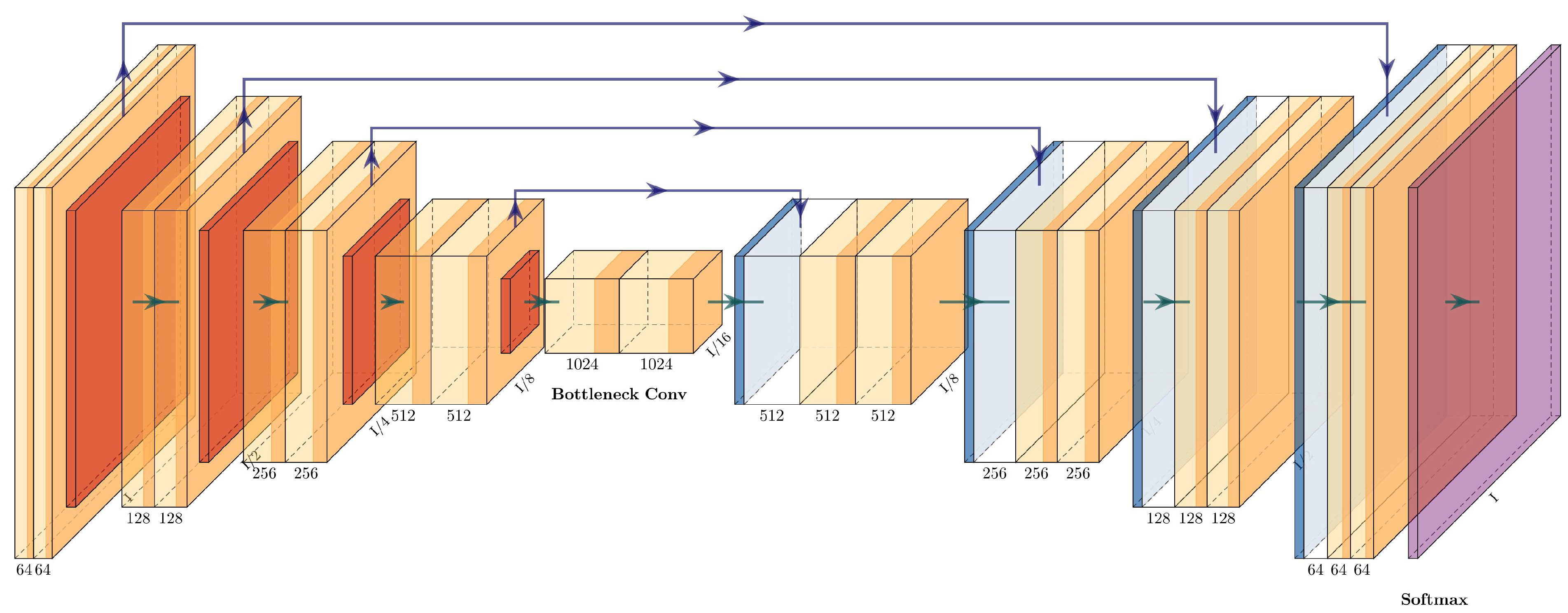
The U-Net architecture has two parts: a contracting path to capture context and an expanding path for localization [19]. The contracting path consists of several blocks of two convolutional layers, followed by a ReLU layer and a max pooling with stride 2. At each downsampling, the number of feature channels is doubled. The expansive paths have several transpose convolution layers for upsampling, a concatenation with the corresponding feature map in the contracting path, and two convolutional layers followed by a ReLU layer. The final layer is a convolutional layer followed by a softmax layer.
The architecture of the classic U-Net can be seen in Figure 7.
3.4.5. PSPNet
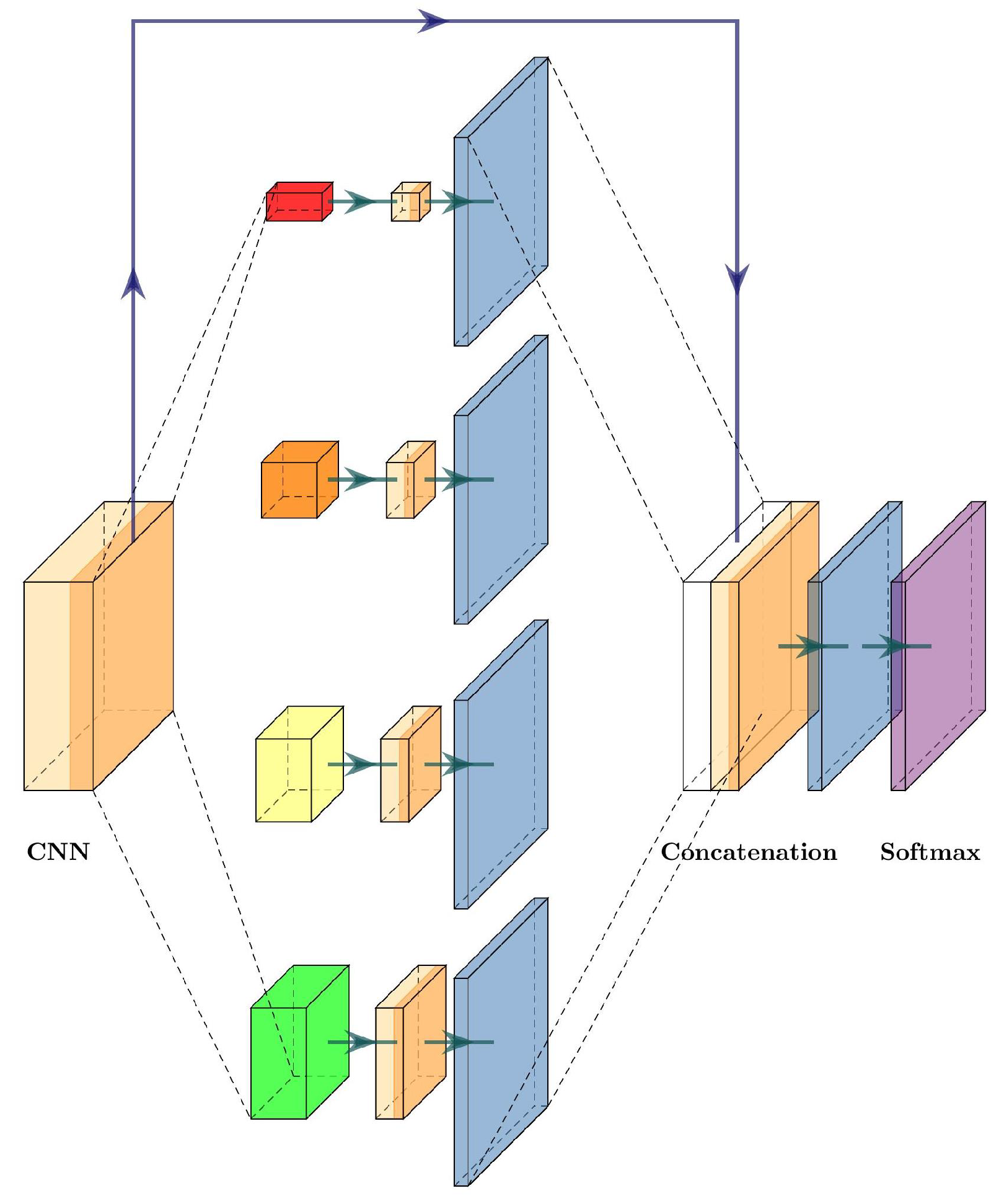
The pyramid scene parsing network (PSPNet) was proposed by Zhao et al. [27] to incorporate suitable global features for semantic segmentation and scene parsing tasks. To obtain global information, PSPNet relies on a pyramid pooling module. This module uses a hierarchical prior, which contains information at different pyramid scales and varying among different sub-regions.
In Figure 8, we can see the pyramid pooling module inside PSPNet. Once the image features are extracted, the multiple pooling layers at several sizes extract global information, and then a convolutional layer is used to flatten the information, followed by an upsampling layer to obtain the original size of the feature map. The final step is to concatenate each feature obtained by the pyramid pooling module, and a convolutional layer generates the final prediction.
3.4.6. VGG16+FCN8
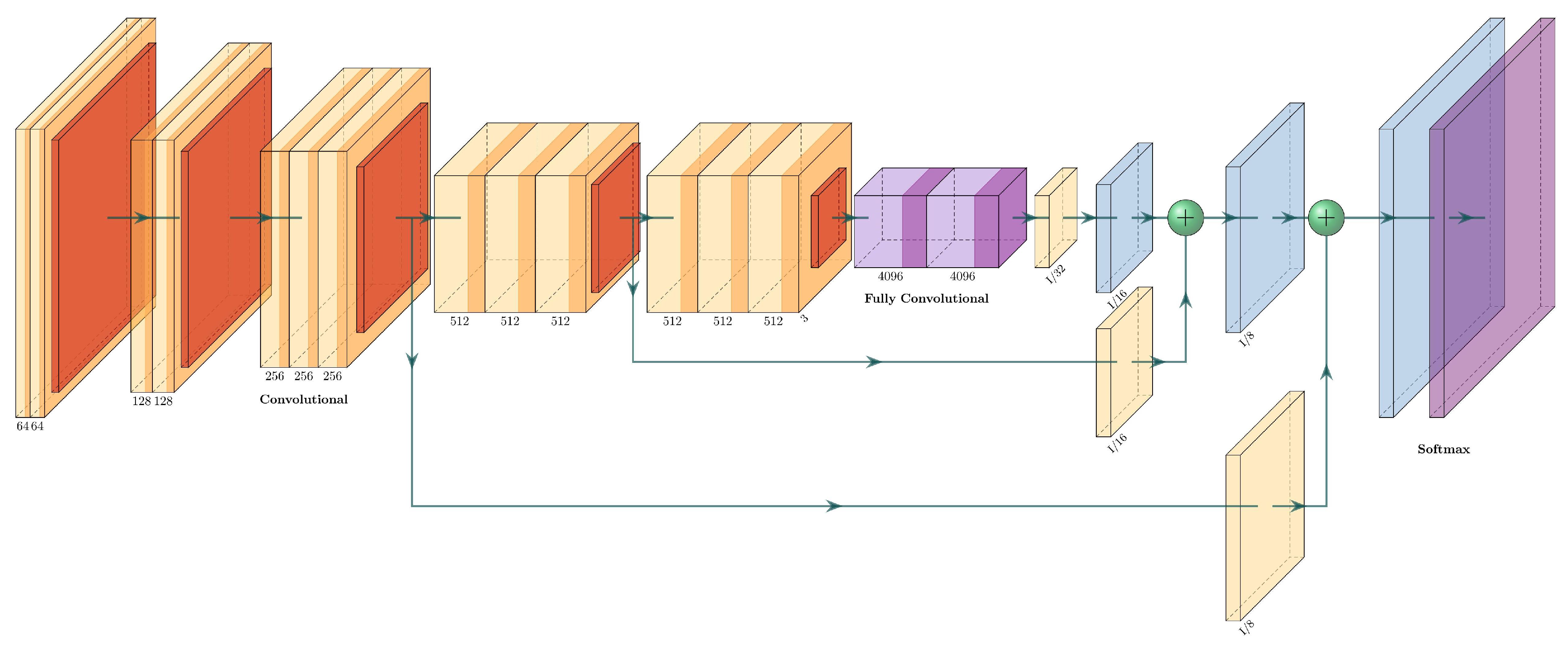
The VGG16+FCN8 is the fully convolutional version of the VGG16. It uses the same architecture as VGG16, but it replaces the two fully connected layers with fully convolutional layers and uses skip connections. This net has three streams before the final upsampling (transposed convolution layer): the output of the fully convolutional layers, a skip connection from pool_4, and a skip connection from pool_3. Every stream passes through a convolutional layer before adding them to the output. The architecture of VGG16+FCN8 can be seen in Figure 9 and is described in Table 3.
3.4.7. VGG16+U-Net
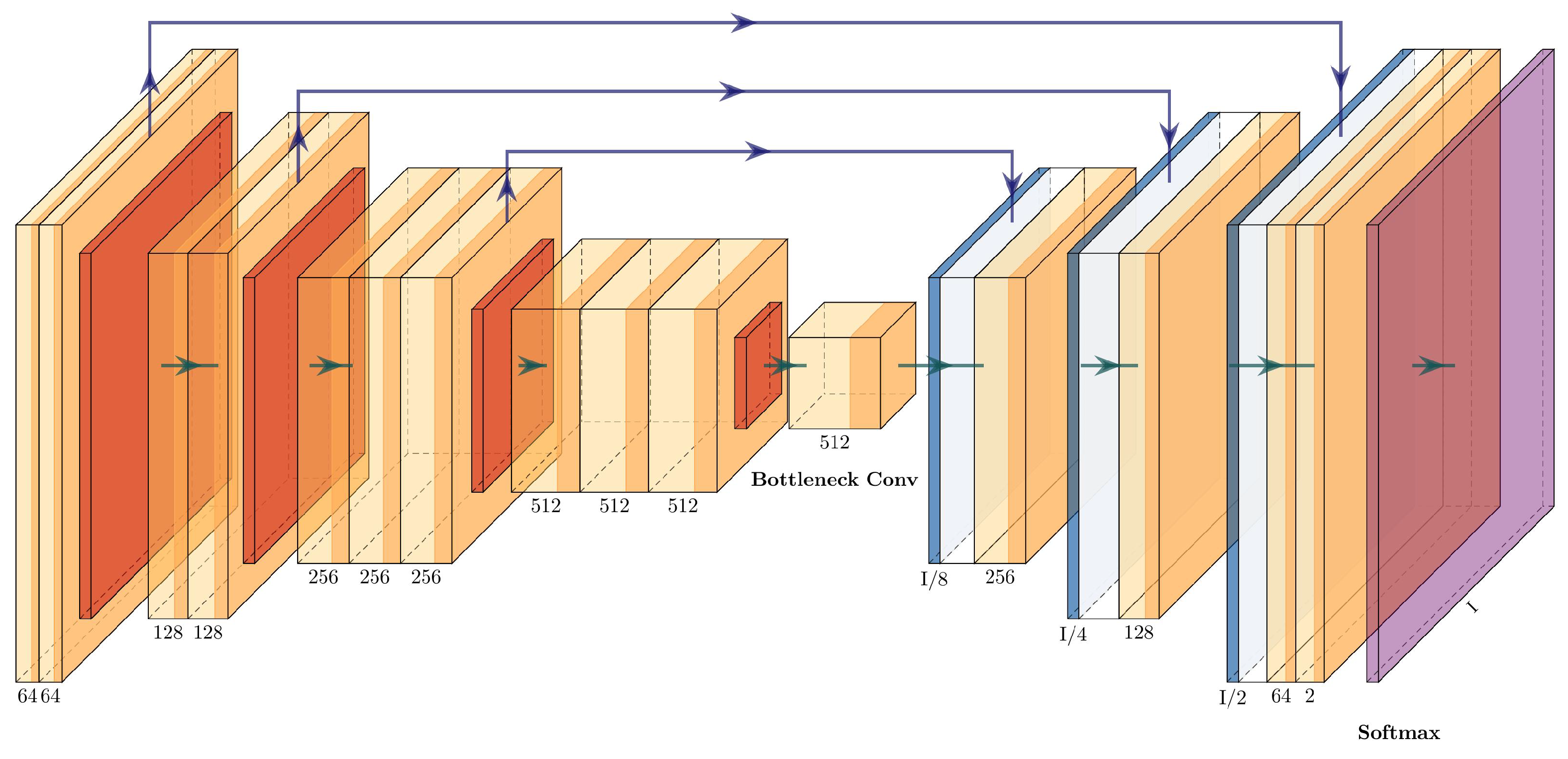
The VGG16+U-Net has the same shape as the U-Net, with a contracting path and an expanding path. The contracting path is integrated by four convolutional blocks of the VGG16 (the last block was removed), with an added single convolutional layer before the expanding path. The expanding path has three upsampling blocks connected with the convolutional blocks. The concatenations between the two paths are performed between Conv_1-Upsampling_3, Conv_2-Upsampling_2, and Conv_3-Upsampling_1. The architecture of the VGG16+U-Net can be seen in Figure 10 and is described in Table 4.
3.4.8. ResNet+PSPNet
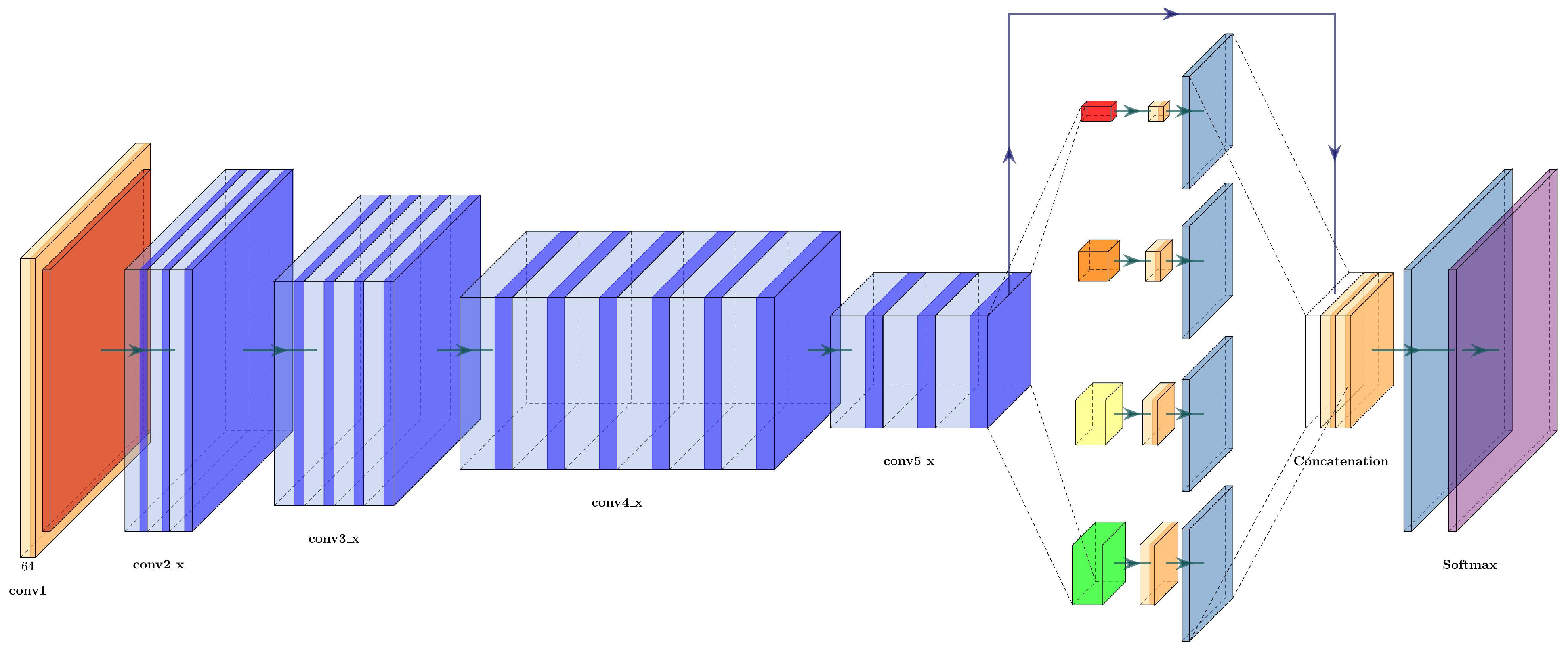
The architecture of the ResNet+PSPNet is simple: it eliminates the fully connected layers of the ResNet50 and adds a pyramid pooling module with two convolutional layers before the final upsampling layers. The last upsampling layer has the same dimension as the first residual block (conv2_x), while the upsampling layers in the pyramid pooling module are half the dimensions of conv5_x. The architecture of ResNet+PSPNet can be seen in Figure 11 and is described in Table 5.
3.4.9. ResNet+U-Net
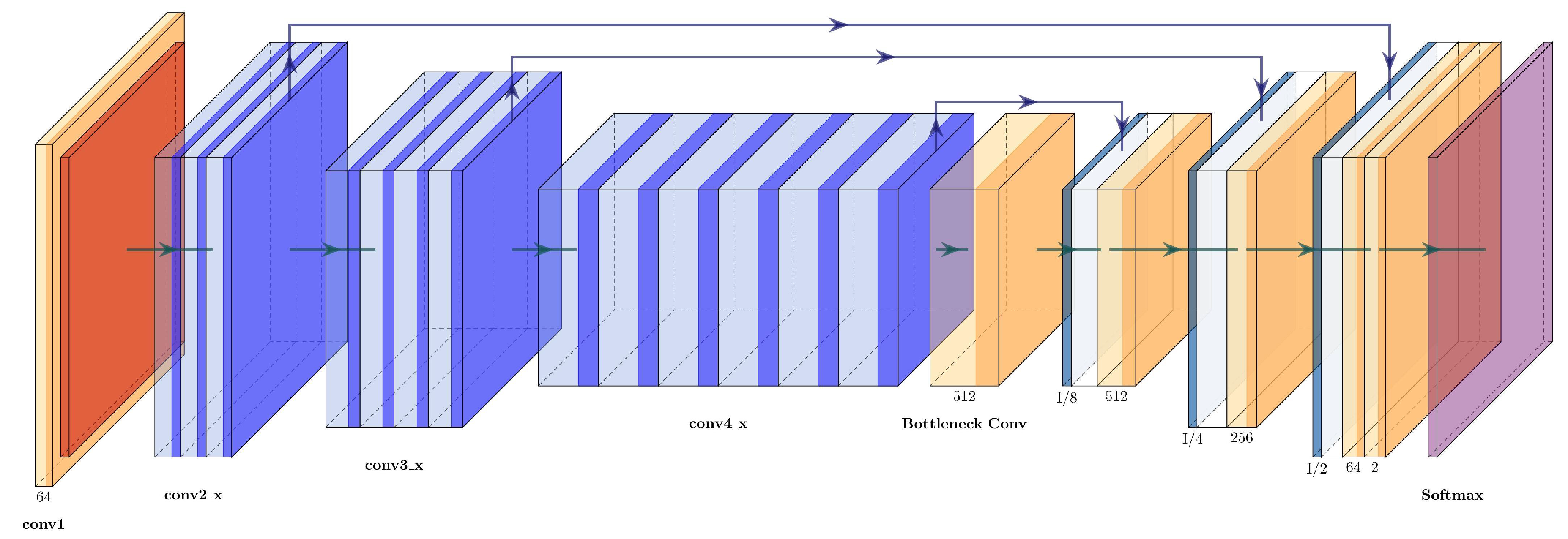
Since VGG16+Unet uses three upsampling blocks in the expanding path, the same number was used for ResNet+U-Net, and only three of the four residual blocks of the original Resnet50 were used for the contracting path. The concatenations between the two paths are carried out between conv2_x-up_3, conv3_x-up_2, and conv4_x-up_1. The architecture of the ResNet50+U-Net can be seen in Figure 12 and is described in Table 6.
3.5. Digitized Mammograms
Mammograms have two standard views: craniocaudal (CC) and mediolateral oblique (MLO). In the CC view, the radiologist has a higher appreciation of the anterior, central, and middle area of the breast [28]. The MLO view complements the CC view; it is taken with an oblique angle, providing a lateral image of the pectoral muscle and the breast. Most of the current research in the automatic segmentation of mammograms focuses on the MLO view. In this view, there are different components, such as the breast region (sometimes divided in fibroglandular tissue and fat), the pectoral muscle, and the nipple.
The breast region is generally more extensive than the pectoral muscle, with a round appearance and most of its pixels near the center or in the mammogram’s lower region. The breast’s gray level intensity depends on its density (the proportion of glandular tissue and fat); the higher the breast’s density, the brighter it appears.
The pectoral muscle is in the upper region of the mammogram. In most cases, the pectoral muscle appears a bright right triangle, with its origin depending on the mammogram’s orientation. The size, brightness, and curvature of the muscle vary on a case-by-case basis [7].
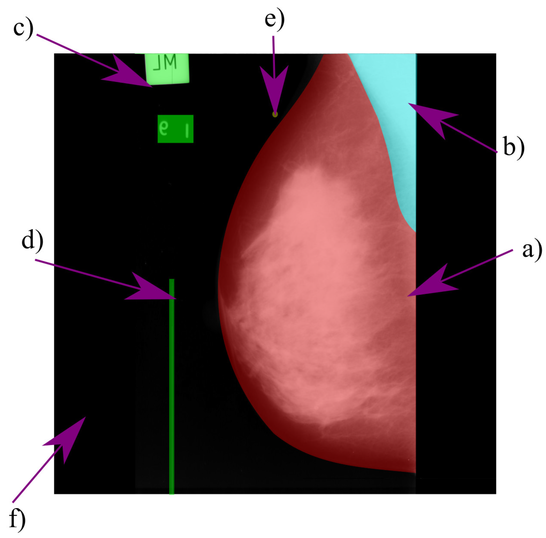
When the mammogram comes from digitized films, it may contain medical labels, noise, and other bright elements that are not part of the breast’s anatomy, e.g., adhesive tape or abnormal spots [3,4,7]. Elements with such characteristics are cataloged as artifacts. Figure 13 shows a typical digitized mammogram and its components.
4. Method
As detailed in Section 2, although deep learning is the dominant technique for segmentation in medical imaging, the number of works that study the performance of architectures for breast segmentation is limited; therefore, the main motivation for this work is to compare the performance of several DNNs in breast segmentation and shed some light on selecting the appropriate network for breast segmentation given the specific purpose.
Modern nets have a better overall performance for multi-label segmentation, but this does not necessarily reflect higher performance on classes with lower pixel-count or classes that resemble geometric shapes (such as the pectoral muscle and breast).
To address all these questions, we performed experiments with four different DNNs: VGG16+FCN8, VGG16+U-Net, ResNet+PSPNet, and ResNet+UNet. The experiments are designed to study the segmentation quality in “One” vs. “All scenario” and “multi-class scenario”, then measure how well the smaller class (the pectoral muscle) is identified.
The selected dataset was the mini-MIAS database [29]. The database has a total of 322 images of digitized mammograms, with a resolution of 200 microns and a size of 1024 × 1024 pixels. To train the networks, we used the labels provided by Oliver et al. [30]. The images are labeled in three classes: breast region, pectoral muscle, and background.
Since the pectoral muscle is much smaller than the breast region (and sometimes does not appear), and the amount of artifacts varies widely between the images, a set of four different training batches was developed.
For the first two experiments, the “One” vs. “All approach” was used. In the first experiment, the pectoral muscle was segmented, and all the other pixels were seen as the background. For the second experiment, the breast region was segmented, with the other classes set as background. In the third experiment, the breast area was identified as the union of the pectoral muscle and the breast region, segmented from the background. The three classes (breast region, pectoral muscle, and background) were segmented individually for the final experiments.
All the experiments used identical hyper-parameters. Each net was trained for 100 epochs using the Adam optimizer with an initial learning rate of and an exponential decay adjusted to achieve a in the last epoch.
Since the amount of training examples is small (only 322 image), dividing the set into training, validation, and testing sets could be prone to overfitting, or it will not assess the performance of the models correctly. A common way to solve this issue is to use K-fold cross-validation in which a set is divided randomly into K batches of examples and trained with batches and leave one for testing. The process is repeated K times, always leaving a different fold as testing set. This means that each training example is used times as part of the training set, and 1 time as part of the test set. Accuracy metrics are calculated for each individual test set, and the average is reported. Since K-fold cross validation averages the performance of the model over all the data, there is a higher confidence in the evaluation of the model.
We used 5-fold cross-validation to evaluate each architecture’s performance; this means of the dataset (64 images) is selected randomly as a test set and the other (258 images) for training. Thus, the model is trained five times, in which each time, the training set and test set are different. Additionally, we used data augmentation in the training process that consisted of a random crop, rotation, translation, padding, and shear. All the networks were trained on a Titan X GPU with 12 GB of RAM.
5. Results
To measure the performance of each architecture, we used two similarity metrics. The first metric is the Jaccard index, also known as the Intersection over Union [31], which is defined as the cardinality of the intersection of two sets divided by the cardinality of the union of the same sets, see Equation (9). The second metric is the SØrensen–Dice (shortened to Dice) coefficient, which is equal to twice the cardinality of the intersection of both sets divided by the number of elements of both sets, see Equation (10).
The experiments were labeled as A (pectoral muscle vs. all), B (breast region vs. all), C (breast area vs. background), and D (three class segmentation). Table 7 and Table 8 indicate the mean value of the 5-fold cross-validation for both segmentation metrics. The columns are labeled PM for pectoral muscle, BC for background, BR for breast region interest, and BR+PM refers to the breast area, including the breast region of interest and the pectoral muscle.
In experiment A, ResNet+PSPNet had the highest Dice coefficient for pectoral muscle segmentation, followed by VGG+FCN8, Resnet+U-Net, and VGG+U-Net. For experiment B, ResNet+U-Net had the highest Dice coefficient, followed by VGG+FCN8, VGG+U-Net, and Resnet+PSPNet. In both experiments, the VGG+FCN8 had the second-best performance differing 0.2% from the best reported in the experiment in A, and 0.12% from the best DNN in experiment B.
As the results for experiment B indicate, all the nets have very similar performance ( 0.98 Dice) for breast region segmentation. The main difference in the performance of the architecture comes when segmenting the pectoral muscle of dense mammograms.
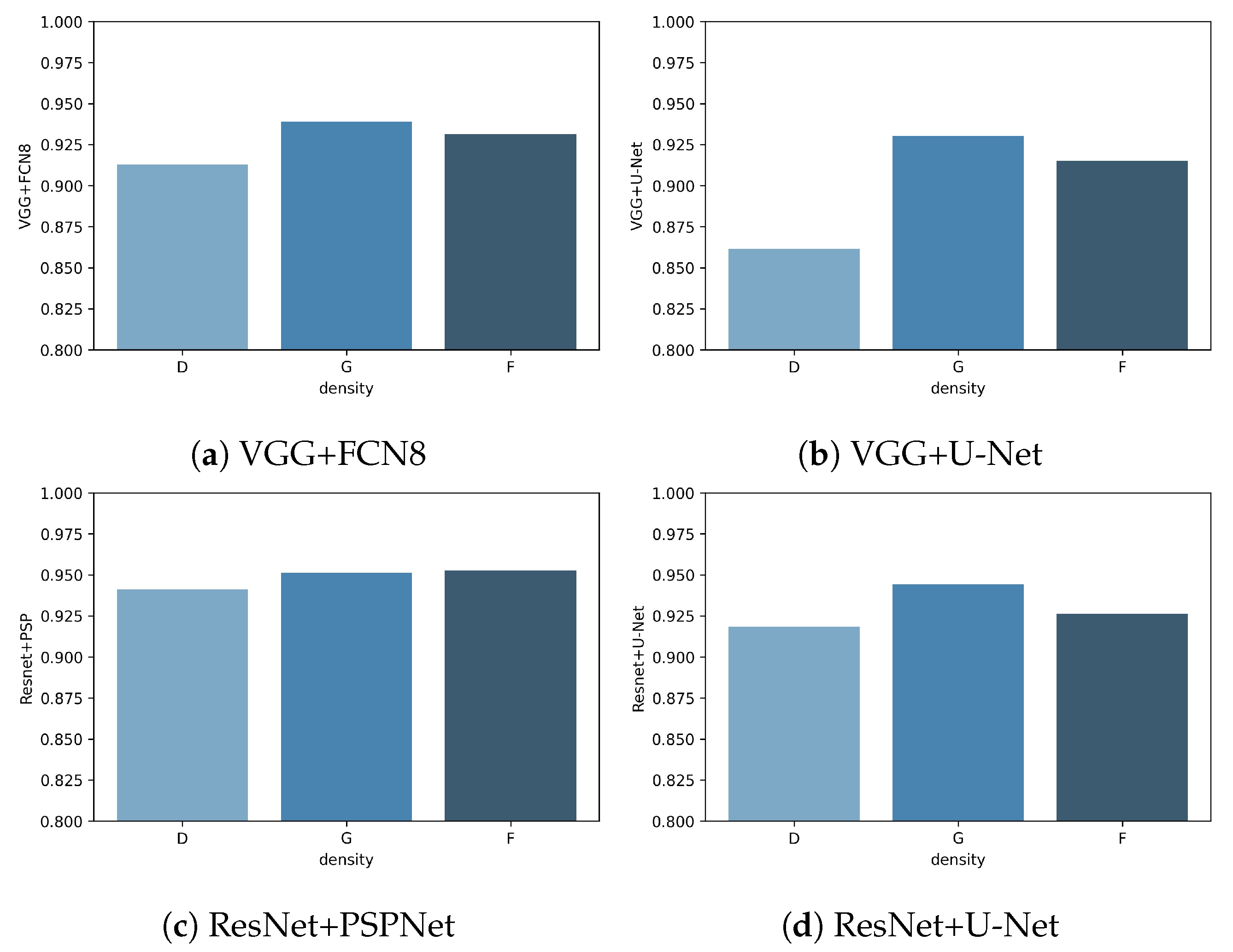
With the density parameter in the mini-MIAS database, we obtained the performance for each density class in experiment A. The three density classes in the mini-MIAS database are F (fatty), G (fatty-glandular), and D (dense-glandular), and the results for each class can be seen in Figure 14.
Class D had the lowest Jaccard metric in every net, while G class had the highest Jaccard index. The best net all-around was ResNet+PSPNet, which has very similar results for every class and achieves the highest value for each class. The most significant difference between classes is observed in VGG+U-Net in which the difference between class D and class G is almost .
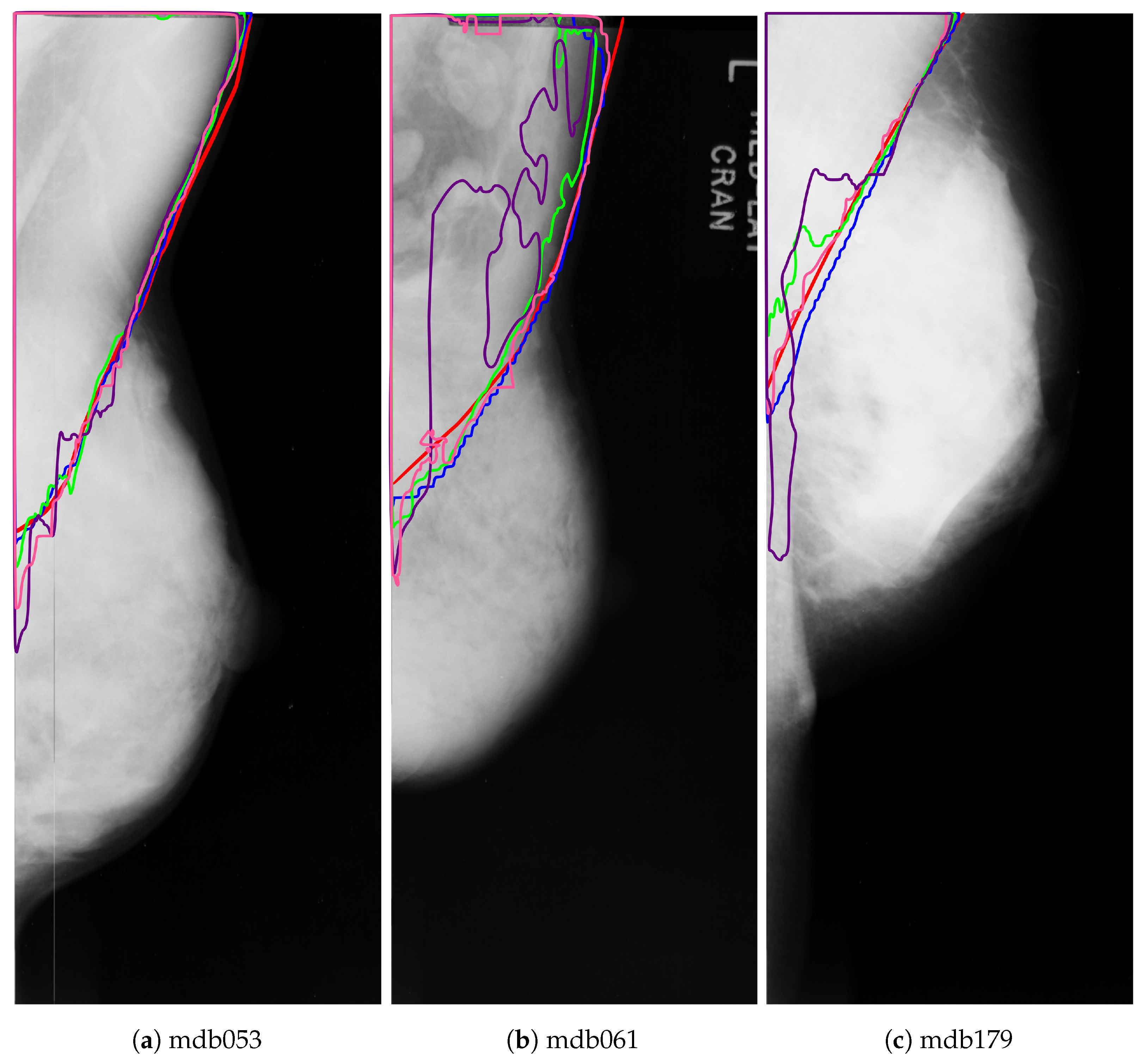
Dense mammograms have the highest amount of error for all the nets, but it is higher for the two U-Net based nets. Figure 15 shows the outline of the pectoral muscle on three dense breasts. As can be seen, both VGG+FCN8 (in pink) and ResNet+PSPNet (in blue) have an outline very similar to the ground truth. Although ResNet+PSPNet (in green) seems to overshoot the pectoral line in Figure 15b,c, the shape of the pectoral line is more natural than the line attained by VGG+FCN8. In the case of Resnet+U-Net, it tends to under-segment the pectoral muscle with an unnatural shape in the lower part of the pectoral region. Finally, VGG+U-Net (in purple) does not perform well for very dense mammograms and generates the most unnatural pectoral line of all the architectures.
The Jaccard index and Dice coefficient are higher in experiments C than those on B, near 0.99 Dice in all the architectures, but with similar ranking in between networks. In experiment D, the breast region segmentation is almost identical to experiment B, with lower performance for the muscle segmentation than in experiment A and better background segmentation.
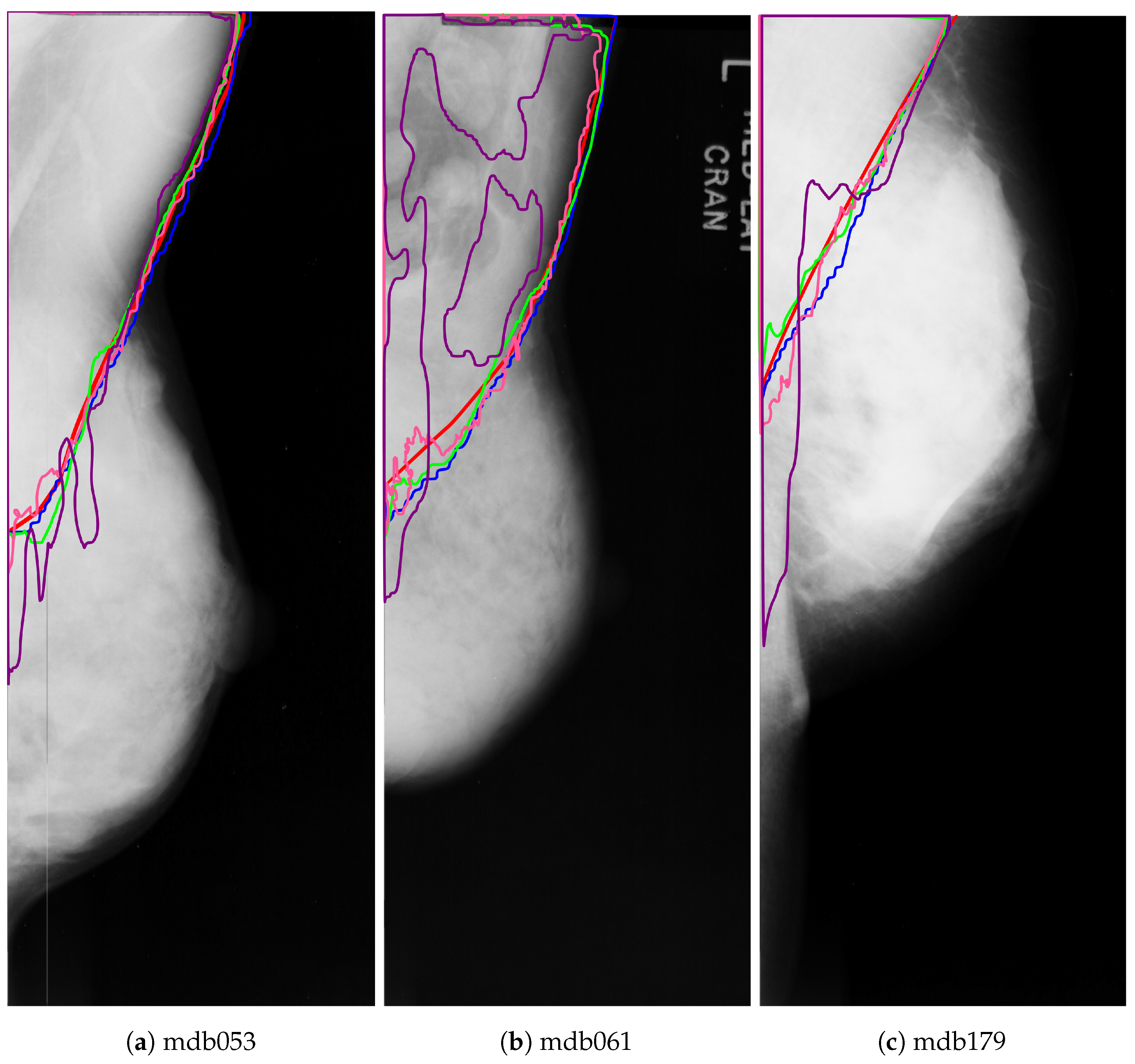
The reduction in the Jaccard and Dice metrics for the pectoral muscle class in experiment D is more evident in dense mammograms, as Figure 16 shows.
From all of the experiments, there are interesting observations to be made. As the results show, U-Net based architectures do not perform well in classes with low pixel-count and have a lower performance with shallower nets. U-Net’s performance was maximized in bigger classes and deeper nets, as indicated by experiments B and C where it achieved the highest results of all the tested architectures. Although, ResNet+PSPNet is a more modern architecture, VGG+FCN8 outperformed it in the breast class in every experiment. On the other hand, the best performance for the low pixel-count class (pectoral muscle) was obtained by ResNet+PSPNet, as indicated in experiments A and D.
We compared the results of the best architectures with different state-of-the-art segmentation approaches, and they are summarized in Table 9. For the breast area segmentation (BR+PM), the best DNN performs better than any other method in the state-of-the-art, which is not surprising since the breast area has a high pixel count and can be easily segmented by a DNN.
For the breast area (BR), the results are also higher than the other two methods compared. In the pectoral muscle, the best DNN was 2.6% below the best method, achieving 0.9545 compared to the 0.98 of the best result in the state-of-the-art.
Multiple Objective Evaluation
The performance of the implemented architectures does not provide a definitive answer on which network performs the best under the tested conditions. A way to balance these results is to test other important features on deep architectures, such as temporal and spatial requirements. The aforementioned can be achieved by trying to maximize the accuracy metrics and minimize the inference time and memory requirements for each network. This approach is an example of a multiobjective optimization problem (MOP) since we are trying to find a compromise between the computational resources and the segmentation metrics of each network.
Multiobjective optimization relies on concepts such as Pareto optimal set and Pareto front [34]. A vector of decision variables is a Pareto optimal if there is no other such that for all and for at least one j. In this definition, the feasible region is represented by . In MOP, it is common to have a set of solutions called the Pareto optimal set [34]. The vectors of this set are called nondominated solutions. A vector of solution is said to dominate , , if and only if . Using this nomenclature, the Pareto optimal set, , can be defined as:
The representation of the nondominated vectors included in the Pareto optimal set is called the Pareto front, which can be represented as:
For calculating the trade-off between different experiments and the temporal and spatial requirements, we use a similar approach as in [35]. The idea is to rank each network in a Pareto front, taking into account the performance in each parameter. We calculated the inference time in seconds and the memory in megabytes for a standard inference on an image; the results can be seen in Table 10. At first glance, VGG16+U-Net requires less time to do an inference and less memory than the others networks, while VGG16+FCN8 took the most time for an inference (0.1445 s), and ResNet+U-Net needed the most memory (1057 MB).
To rank the solutions, we base on the distance between the solutions. Since in some experiments, the distance between metrics is minimal, we established a difference of at least 1% between each parameter was enough to indicate that one network dominated over another and they had a lower rank. The results can be seen in Table 11.
The ranking in Table 11 corroborates the previous findings: the best-performing networks taking only into consideration the accuracy metrics are VGG+FCN8 and ResNet+U-Net; however, if we consider the results of inference time and memory needed for each network, the best performing architecture is Resnet+PSPNet followed by VGG+U-Net. The results of the ranking systems are important on limited since the expert can decide to use a network that does not yield the best results but overall has good performance metrics and a lower computational power to implement.
6. Discussion and Future Work
This paper proposes an extensive analysis of mammogram semantic segmentation using DNNs. Four different encoder–decoder pairs were trained and evaluated in four different experimental setups.
Our results show that all the architectures perform well (near 0.99 in Dice) for breast border segmentation, with higher results than state-of-the-art approaches. For breast region segmentation, all the architectures had a Dice metric superior to 0.98.
The highest variation was attained in the experiments that included the isolation of the pectoral muscle. The two architectures that use the U-Net segmentation approach have the smallest Dice value, surpassed by a very shallow net such as VGG16+FCN8. This issue is transcendental since U-Net is the go-to architecture for semantic segmentation for many medical imaging articles. Our research work reveals that other architectures may obtain higher performance for classes with low pixel-count in medical images.
The highest variation was due to breast density for the pectoral muscle segmentation since the lowest Dice coefficient was obtained in dense mammograms in all four architectures; however, ResNet+PSPNet had very similar results for the three classes proving to be the best architecture for low pixel-count classes in mammograms. The main drawback was its performance on the breast region class, where it had the worst Dice metric of all the architectures.
Our results indicate that the trained DNNs have good performance for mammogram segmentation. The best combination for mammogram segmentation seems to be a union of the output of the breast line given by ResNet+U-Net and the pectoral segmentation given by ResNet+PSPNet.
The multiobjective evaluation of memory and time requirements showed the importance of balancing the best performance against these two parameters. This evaluation indicates that ResNet+PSPNet has a good balance between accuracy metrics and computational requirements. The second-best overall network was VGG16+UNet, but their lower performance in dense mammograms does not make this network appealing in those cases.
In future work, the influence of different and more depth feature extraction architectures can be explored. A balance between the segmentation of low pixel-count and high pixel-count classes might be achieved by a pyramid module embedded on a U-shaped segmentation net; this could balance between the good performance and capacity of training with small databases of the U-Net, and the accuracy of detecting low pixel-count classes of PSPNet.
Author Contributions
Conceptualization, Y.R. and O.M.; methodology, Y.R. and O.M; software, Y.R.; validation, Y.R., O.M.; formal analysis, Y.R. and O.M.; investigation, Y.R. and O.M.; resources, O.M.; data curation, Y.R.; writing—original draft preparation, Y.R. and O.M.; writing—review and editing, Y.R. and O.M.; visualization, Y.R. and O.M.; supervision, O.M.; project administration, O.M.; funding acquisition, O.M. Both authors have read and agreed to the published version of the manuscript.
Funding
This research was funded by Instituto Politécnico Nacional (grant number SIP2020053) and the Mexican National Council of Science and Technology (CONACYT).
Conflicts of Interest
The authors declare no conflict of interest.
References
- Nagi, J.; Kareem, S.; Nagi, F.; Ahmed, S. Automated breast profile segmentation for ROI detection using digital mammograms. In Proceedings of the 2010 IEEE EMBS Conference on Biomedical Engineering and Sciences (IECBES), Kuala Lumpur, Malaysia, 30 November–2 December 2010; pp. 87–92. [Google Scholar] [CrossRef]
- Taghanaki, S.A.; Liu, Y.; Miles, B.; Hamarneh, G. Geometry-Based Pectoral Muscle Segmentation From MLO Mammogram Views. IEEE Trans. Biomed. Eng. 2017, 64, 2662–2671. [Google Scholar]
- Rampun, A.; Morrow, P.J.; Scotney, B.W.; Winder, J. Fully automated breast boundary and pectoral muscle segmentation in mammograms. Artif. Intell. Med. 2017, 79, 28–41. [Google Scholar] [CrossRef] [Green Version]
- Dubrovina, A.; Kisilev, P.; Ginsburg, B.; Hashoul, S.; Kimmel, R. Computational mammography using deep neural networks. Comput. Methods Biomech. Biomed. Eng. Imaging Vis. 2018, 6, 243–247. [Google Scholar] [CrossRef]
- Mustra, M.; Grgic, M. Robust automatic breast and pectoral muscle segmentation from scanned mammograms. Signal Process. 2013, 93, 2817–2827. [Google Scholar] [CrossRef]
- Kwok, S.M.; Chandrasekhar, R.; Attikiouzel, Y.; Rickard, M.T. Automatic pectoral muscle segmentation on mediolateral oblique view mammograms. IEEE Trans. Med. Imaging 2004, 23, 1129–1140. [Google Scholar] [CrossRef] [Green Version]
- Vikhe, P.S.; Thool, V.R. Detection and Segmentation of Pectoral Muscle on MLO-View Mammogram Using Enhancement Filter. J. Med. Syst. 2017, 41, 1–13. [Google Scholar] [CrossRef] [PubMed]
- Liu, L.; Liu, Q.; Lu, W. Pectoral Muscle Detection in Mammograms Using Local Statistical Features. J. Digit. Imaging 2014, 27, 633–641. [Google Scholar] [CrossRef] [PubMed] [Green Version]
- Gastounioti, A.; Conant, E.; Kontos, D. Beyond breast density: A review on the advancing role of parenchymal texture analysis in breast cancer risk assessment. Breast Cancer Res. 2016, 18, 243–247. [Google Scholar] [CrossRef] [Green Version]
- Hesamian, M.H.; Jia, W.; He, X.; Kennedy, P. Deep Learning Techniques for Medical Image Segmentation: Achievements and Challenges. J. Digit. Imaging 2019, 32, 582–596. [Google Scholar] [CrossRef] [Green Version]
- de Oliveira, H.; Correa Machado, C.D.A.; de Albuquerque Araujo, A. Exploring Deep-Based Approaches for Semantic Segmentation of Mammographic Images. In Progress in Pattern Recognition, Image Analysis, Computer Vision, and Applications; Lecture Notes in Computer Science; Springer: Cham, Switzerland, 2019; pp. 691–698. [Google Scholar] [CrossRef]
- Litjens, G.; Kooi, T.; Bejnordi, B.E.; Setio, A.A.A.; Ciompi, F.; Ghafoorian, M.; van der Laak, J.A.; van Ginneken, B.; Sánchez, C.I. A survey on deep learning in medical image analysis. Med. Image Anal. 2017, 42, 60–88. [Google Scholar] [CrossRef] [PubMed] [Green Version]
- Dalmış, M.U.; Litjens, G.; Holland, K.; Setio, A.; Mann, R.; Karssemeijer, N.; Gubern-Mérida, A. Using deep learning to segment breast and fibroglandular tissue in MRI volumes. Med. Phys. 2017, 44, 533–546. [Google Scholar] [CrossRef]
- Rampun, A.; López-Linares, K.; Morrow, P.J.; Scotney, B.W.; Wang, H.; Ocaña, I.G.; Maclair, G.; Zwiggelaar, R.; Ballester, M.A.G.; Macía, I. Breast pectoral muscle segmentation in mammograms using a modified holistically-nested edge detection network. Med. Image Anal. 2019, 57, 1–17. [Google Scholar] [CrossRef]
- Ahmed, L.; Aldabbas, M.; Aldabbas, H.; Khalid, S.; Saleem, Y.; Saeed, S. Images data practices for Semantic Segmentation of Breast Cancer using Deep Neural Network. J. Ambient. Intell. Humaniz. Comput. 2020. [Google Scholar] [CrossRef]
- Lecun, Y.; Bottou, L.; Bengio, Y.; Haffner, P. Gradient-based learning applied to document recognition. Proc. IEEE 1998, 86, 2278–2324. [Google Scholar] [CrossRef] [Green Version]
- Lin, M.; Chen, Q.; Yan, S. Network in Network. arXiv 2014, arXiv:1312.4400. [Google Scholar]
- Shelhamer, E.; Long, J.; Darrell, T. Fully Convolutional Networks for Semantic Segmentation. IEEE Trans. Patter Recognit. Mach. Intell. 2017, 39, 640–651. [Google Scholar] [CrossRef] [PubMed]
- Ronneberger, O.; Fischer, P.; Brox, T. U-Net: Convolutional Networks for Biomedical Image Segmentation. In Medical Image Computing and Computer-Assisted Intervention (MICCAI); Springer: Berlin/Heidelberg, Germany, 2015; Volume 9351, pp. 234–241. [Google Scholar]
- Jégou, S.; Drozdzal, M.; Vazquez, D.; Romero, A.; Bengio, Y. The One Hundred Layers Tiramisu: Fully Convolutional DenseNets for Semantic Segmentation. In Proceedings of the 2017 IEEE Conference on Computer Vision and Pattern Recognition Workshops (CVPRW), Honolulu, HI, USA, 21–26 July 2017; pp. 1175–1183. [Google Scholar] [CrossRef] [Green Version]
- Chen, L.C.; Papandreou, G.; Kokkinos, I.; Murphy, K.; Yuille, A.L. DeepLab: Semantic Image Segmentation with Deep Convolutional Nets, Atrous Convolution, and Fully Connected CRFs. arXiv 2016, arXiv:1606.00915. [Google Scholar] [CrossRef] [PubMed]
- Chen, L.C.; Papandreou, G.; Schroff, F.; Adam, H. Rethinking Atrous Convolution for Semantic Image Segmentation. arXiv 2017, arXiv:1706.05587. [Google Scholar]
- Chen, L.C.; Zhu, Y.; Papandreou, G.; Schroff, F.; Adam, H. Encoder-Decoder with Atrous Separable Convolution for Semantic Image Segmentation. In Computer Vision–ECCV 2018; Ferrari, V., Hebert, M., Sminchisescu, C., Weiss, Y., Eds.; Springer International Publishing: Cham, Swizterland, 2018; pp. 833–851. [Google Scholar] [CrossRef] [Green Version]
- Siam, M.; Gamal, M.; Abdel-Razek, M.; Yogamani, S.; Jagersand, M.; Zhang, H. A Comparative Study of Real-Time Semantic Segmentation for Autonomous Driving. In Proceedings of the 2018 IEEE/CVF Conference on Computer Vision and Pattern Recognition Workshops (CVPRW), Salt Lake City, UT, USA, 18–22 June 2018; pp. 700–710. [Google Scholar]
- Simonyan, K.; Zisserman, A. Very Deep Convolutional Networks for Large-Scale Image Recognition. In Proceedings of the International Conference on Learning Representations, San Diego, CA, USA, 7–9 May 2015. [Google Scholar]
- He, K.; Zhang, X.; Ren, S.; Sun, J. Deep Residual Learning for Image Recognition. In Proceedings of the 2016 IEEE Conference on Computer Vision and Pattern Recognition (CVPR), Las Vegas, NV, USA, 27–30 June 2016; pp. 770–778. [Google Scholar]
- Zhao, H.; Shi, J.; Qi, X.; Wang, X.; Jia, J. Pyramid Scene Parsing Network. In Proceedings of the 2017 IEEE Conference on Computer Vision and Pattern Recognition (CVPR), Honolulu, HI, USA, 21–26 July 2017; pp. 6230–6239. [Google Scholar]
- Radhakrishna, S. Breast Diseases, 1st ed.; Springer: Chennai, India, 2015. [Google Scholar] [CrossRef]
- Suckling, J.; Parker, J.; Dance, D.; Astley, S. The Mammographic Image Analysis Society Digital Mammogram Database. Exerpta Medica. Int. Congr. Ser. 1994, 1069, 375–378. [Google Scholar]
- Oliver, A.; Lladó, X.; Torrent, A.; Martí, J. One-shot segmentation of breast, pectoral muscle, and background in digitised mammograms. In Proceedings of the 2014 IEEE International Conference on Image Processing (ICIP), Paris, France, 27–30 October 2014; pp. 912–916. [Google Scholar] [CrossRef]
- Jaccard, P. The distribution of the flora in the Alpine zone. New Phytol. 1912, 11, 37–50. [Google Scholar] [CrossRef]
- Olsen, C.M. Automatic breast border extraction. In Medical Imaging 2005: Image Processing; Fitzpatrick, J.M., Reinhardt, J.M., Eds.; International Society for Optics and Photonics, SPIE: Bellingham, WA, USA, 2005; Volume 5747, pp. 1616–1627. [Google Scholar] [CrossRef]
- Shen, R.; Yan, K.; Xiao, F.; Chang, J.; Jiang, C.; Zhou, K. Automatic Pectoral Muscle Region Segmentation in Mammograms Using Genetic Algorithm and Morphological Selection. J. Digit. Imaging 2018, 31, 680–691. [Google Scholar] [CrossRef] [PubMed]
- Coello, C.; Lamont, G.; van Veldhuizen, D.A. Evolutionary Algorithms for Solving Multi-Objective Problems; Springer: Berlin/Heidelberg, Germany, 2007. [Google Scholar] [CrossRef]
- Olvera, C.; Rubio, Y.; Montiel, O. Multi-objective Evaluation of Deep Learning Based Semantic Segmentation for Autonomous Driving Systems. In Intuitionistic and Type-2 Fuzzy Logic Enhancements in Neural and Optimization Algorithms: Theory and Applications; Castillo, O., Melin, P., Kacprzyk, J., Eds.; Springer International Publishing: Cham, Swizterland, 2020; pp. 299–311. [Google Scholar] [CrossRef]
Figure 1.
Example of a convolutional operation.

Figure 2.
Example of max pooling and average pooling.

Figure 3.
Architecture of the VGG-16.

Figure 4.
ResNets address the accuracy saturation and accuracy degradation issue with residual blocks. (a) Traditional DNN stacking where each layer feeds into the next layer. (b) In residual blocks the output of a layers is added to a layer deeper in the block.
Figure 4.
ResNets address the accuracy saturation and accuracy degradation issue with residual blocks. (a) Traditional DNN stacking where each layer feeds into the next layer. (b) In residual blocks the output of a layers is added to a layer deeper in the block.

Figure 5.
Architecture of the ResNet50.

Figure 6.
Architecture of the FCN-8 of a generic DNN.

Figure 7.
Architecture of the U-Net.

Figure 8.
Pyramid pooling module.

Figure 9.
Architecture of the VGG16+FCN8.

Figure 10.
Architecture of the VGG16+U-Net.

Figure 11.
Architecture of the ResNet50+PSPNet.

Figure 12.
Architecture of the ResNet50+U-Net.

Figure 13.
Typical components of a digitized mammogram: (a) breast region, (b) pectoral muscle, (c) medical label, (d) digitization artifact, (e) salt noise, and (f) background.
Figure 13.
Typical components of a digitized mammogram: (a) breast region, (b) pectoral muscle, (c) medical label, (d) digitization artifact, (e) salt noise, and (f) background.

Figure 14.
Jaccard index for each architecture by density class.

Figure 15.
Pectoral muscle segmentation for the different DNNs: ground truth (red), ResNet50+PSPNet (blue), ResNet50+U-Net (green), VGG+FCN8 (pink), and VGG+U-Net (purple).
Figure 15.
Pectoral muscle segmentation for the different DNNs: ground truth (red), ResNet50+PSPNet (blue), ResNet50+U-Net (green), VGG+FCN8 (pink), and VGG+U-Net (purple).

Figure 16.
Pectoral muscle segmentation for the dense class using the different DNNs: ground truth (red), ResNet50+PSPNet (blue), ResNet50+U-Net (green), VGG+FCN8 (pink), and VGG+U-Net (purple).
Figure 16.
Pectoral muscle segmentation for the dense class using the different DNNs: ground truth (red), ResNet50+PSPNet (blue), ResNet50+U-Net (green), VGG+FCN8 (pink), and VGG+U-Net (purple).


Table 1.
Layer description of the VGG16.
| Type | Filters | Size, Stride |
|---|---|---|
| Conv_1 | 64 × 2 | , 1 |
| Pool_1 | – | 2 |
| Conv_2 | 128 × 2 | , 1 |
| Pool_2 | – | 2 |
| Conv_3 | 256 × 3 | , 1 |
| Pool_3 | – | 2 |
| Conv_4 | 512 × 3 | , 1 |
| Pool_4 | – | 2 |
| Conv_5 | 512 × 3 | , 1 |
| Pool_5 | – | 2 |
| FConv | 4096 | |
| FConv | 4096 | |
| Softmax | – | – |
Table 2.
Layer description of ResNet50.
| Type | Filters | Size, Stride |
|---|---|---|
| Conv_1 | 64 | , 2 |
| Pool_1 | – | , 2 |
| 64 | , 1 | |
| Conv_2 | 64 | , 1 |
| 256 | , 1 | |
| 128 | , 1 | |
| Conv_3 | 128 | , 1 |
| 512 | , 1 | |
| 256 | , 1 | |
| Conv_4 | 256 | , 1 |
| 1024 | , 1 | |
| 512 | , 1 | |
| Conv_5 | 512 | , 1 |
| 2048 | , 1 | |
| GAP | – | |
| Softmax | – | – |
Table 3.
Layer description of the VGG16+FCN8.
| Type | Filters | Conected to |
|---|---|---|
| VGG16 | – | – |
| Conv_6 × 2 | 4096 | Conv_5 |
| Conv_7 | 2 | Conv_6 |
| TransConv_1 | 1 | Conv_7 |
| Conv_8 | 1 | Pool_4 |
| Add_1 | – | – |
| TransConv_2 | 1 | Add_1 |
| Conv_9 | 1 | Pool_4 |
| Add_2 | – | – |
| TransConv_3 | 1 | Add_2 |
| Softmax | – | TransConv_3 |
Table 4.
Layer description of the VGG16+U-Net.
| Type | Filters | Conected to |
|---|---|---|
| VGG16 | – | – |
| Conv_5 | 512 | Conv_4 |
| Upsampling_1 | 512 | Conv_5 |
| Concat_1 | 768 | Conv_3 |
| Conv_6 | 256 | Concat_1 |
| Upsampling_2 | 256 | Conv_6 |
| Concat_2 | 384 | Conv_2 |
| Conv_7 | 128 | Concat_2 |
| Upsampling_3 | 128 | Conv_7 |
| Concat_3 | 192 | Upsampling_3 |
| Conv_8 | 64 | Concat_3 |
| Conv_9 | 2 | Conv_8 |
| Softmax | – | Conv_9 |
Table 5.
Layer description of the ResNet50+PSPNet.
| Type | Filters | Conected to |
|---|---|---|
| ResNet50 | – | – |
| AVGPool_1 | 2048 | Conv5_x |
| Conv_6 | 512 | AVGPool_1 |
| Upsampling_1 | 512 | Conv_6 |
| AVGPool_2 | 2048 | Conv5_x |
| Conv_7 | 512 | AVGPool_2 |
| Upsampling_2 | 512 | Conv_7 |
| AVGPool_3 | 2048 | Conv5_x |
| Conv_8 | 512 | AVGPool_3 |
| Upsampling_3 | 512 | Conv_8 |
| AVGPool_4 | 2048 | Conv5_x |
| Conv_9 | 512 | AVGPool_4 |
| Upsampling_4 | 512 | Conv_9 |
| Concat_1 | 4096 | Conv_6 |
| Conv_7 | ||
| Conv_8 | ||
| Conv_9 | ||
| Conv_10 | 512 | Concat_1 |
| Conv_11 | 2 | Conv_10 |
| Softmax | – | Conv_11 |
Table 6.
Layer description of the ResNet50+U-Net.
| Type | Filters | Conected to |
|---|---|---|
| ResNet50 | – | – |
| Conv_5 | 512 | Conv4_x |
| Upsampling_1 | 512 | Conv_5 |
| Concat_1 | 1024 | Conv4_x |
| Conv_6 | 256 | Concat_1 |
| Upsampling_2 | 256 | Conv_6 |
| Concat_2 | 512 | Conv3_x |
| Conv_7 | 128 | Concat_2 |
| Upsampling_3 | 128 | Conv_7 |
| Concat_3 | 192 | Conv2_x |
| Conv_8 | 64 | Concat_3 |
| Conv_9 | 2 | Conv_8 |
| Softmax | – | Conv_9 |
Table 7.
Segmentation metrics for experiments A and B. Best results in bold.
| A | B | |||
|---|---|---|---|---|
| Net | PM | BC | BR | BC |
| VGG+FCN8 | J: 0.8985 D: 0.9465 | J: 0.9888 D: 0.9943 | J: 0.9681 D: 0.9838 | J: 0.9563 D: 0.9777 |
| VGG+U-Net | J: 0.8644 D: 0.9272 | J: 0.9852 D: 0.9925 | J: 0.9641 D: 0.9817 | J: 0.9503 D: 0.9745 |
| ResNet+PSPNet | J: 0.9130 D: 0.9545 | J: 0.9903 D: 0.9951 | J: 0.9627 D: 0.9810 | J: 0.9488 D: 0.9737 |
| ResNet+U-Net | J: 0.8954 D: 0.9448 | J: 0.9885 D: 0.9942 | J: 0.9705 D: 0.9850 | J: 0.9595 D: 0.9793 |
Table 8.
Segmentation metrics for experiments C and D. Best results in bold.
| C | D | ||||
|---|---|---|---|---|---|
| Net | BR+PM | BC | BR | PM | BC |
| VGG+FCN8 | J: 0.9863 D: 0.9931 | J: 0.9715 D: 0.9855 | J: 0.9674 D: 0.9834 | J: 0.8934 D: 0.9437 | J: 0.9701 D: 0.9848 |
| VGG+U-Net | J: 0.9856 D: 0.9927 | J: 0.9697 D: 0.9846 | J: 0.9630 D: 0.9811 | J: 0.8483 D: 0.9179 | J: 0.9656 D: 0.9825 |
| ResNet+PSPNet | J: 0.9798 D: 0.9898 | J: 0.9575 D: 0.9782 | J: 0.9617 D: 0.9805 | J: 0.9024 D: 0.9487 | J: 0.9551 D: 0.9770 |
| ResNet+U-Net | J: 0.9876 D: 0.9937 | J: 0.9741 D: 0.9869 | J: 0.9704 D: 0.9850 | J: 0.8995 D: 0.9471 | J: 0.9734 D: 0.9865 |
Table 9.
Comparison of the best net with other proposals. Best results in bold.
| Method | BR+PM | PM | BR |
|---|---|---|---|
| Best DNN | J: 0.9876 D: 0.9937 | J: 0.9130 D: 0.9545 | J: 0.9705 D: 0.9850 |
| Nagi et al. [1] | J: 0.9236 D: 0.9598 | J: 0.6170 D: 0.7361 | J: ——– D: ——– |
| Mustra and Grgic [5] | J: 0.9525 D: 0.9751 | J: ——– D: ——– | J: ——– D: ——– |
| Olsen [32] | J: 0.9436 D: 0.9704 | J: ——– D: ——– | J: ——– D: ——– |
| Shen et al. [33] | J: ——– D: ——– | J: 0.9125 D: 0.9496 | J: ——– D: ——– |
| Oliver et al. [30] | J: ——– D: 0.9600 | J: ——– D: 0.8300 | J: ——– D: 0.9700 |
| Taghanaki et al. [2] | J: ——– D: ——– | J: 0.9700 D: 0.9800 | J: ——– D: ——– |
| Rampun et al. [3] | J: 0.9760 D: 0.9880 | J: 0.9210 D: 0.9580 | J: 0.9510 D: 0.9730 |
| Rampun et al. [14] | J: ——– D: ——– | J: 0.9460 D: 0.9750 | J: ——– D: ——– |
Table 10.
Temporal and spatial requirements of each architecture.
| Network | Time (s) | Memory (MB) |
|---|---|---|
| VGG16+FCN8 | 0.1445 | 826 |
| VGG16+U-Net | 0.0699 | 613 |
| ResNet+PSPNet | 0.0717 | 727 |
| ResNet+U-Net | 0.0797 | 1057 |
Table 11.
Ranking for every network at a given metric. The experiment is indicated in parenthesis.
| Network | Time | Memory | PM(A) | BR(B) | PM+BR(C) | PM(D) |
|---|---|---|---|---|---|---|
| VGG16+FCN8 | III | III | II | I | I | I |
| VGG16+U-Net | I | I | III | II | I | II |
| ResNet+PSPNet | I | II | I | II | II | I |
| ResNet+U-Net | II | IV | II | I | I | I |
Publisher’s Note: MDPI stays neutral with regard to jurisdictional claims in published maps and institutional affiliations. |
© 2021 by the authors. Licensee MDPI, Basel, Switzerland. This article is an open access article distributed under the terms and conditions of the Creative Commons Attribution (CC BY) license (https://creativecommons.org/licenses/by/4.0/).
Share and Cite
MDPI and ACS Style
Rubio, Y.; Montiel, O. Multicriteria Evaluation of Deep Neural Networks for Semantic Segmentation of Mammographies. Axioms 2021, 10, 180. https://0-doi-org.brum.beds.ac.uk/10.3390/axioms10030180
AMA Style
Rubio Y, Montiel O. Multicriteria Evaluation of Deep Neural Networks for Semantic Segmentation of Mammographies. Axioms. 2021; 10(3):180. https://0-doi-org.brum.beds.ac.uk/10.3390/axioms10030180
Chicago/Turabian StyleRubio, Yoshio, and Oscar Montiel. 2021. "Multicriteria Evaluation of Deep Neural Networks for Semantic Segmentation of Mammographies" Axioms 10, no. 3: 180. https://0-doi-org.brum.beds.ac.uk/10.3390/axioms10030180
Note that from the first issue of 2016, this journal uses article numbers instead of page numbers. See further details here.