
Cheap Control in a Non-Scalarizable Linear-Quadratic Pursuit-Evasion Game: Asymptotic Analysis

1
Department of Mathematics, Ort Braude College of Engineering, 51 Snunit Str., P.O. Box 78, Karmiel 2161002, Israel
2
The Galilee Research Center for Applied Mathematics, Ort Braude College of Engineering, 51 Snunit Str., P.O. Box 78, Karmiel 2161002, Israel
*
Author to whom correspondence should be addressed.
†
These authors contributed equally to this work.
Axioms 2022, 11(5), 214; https://0-doi-org.brum.beds.ac.uk/10.3390/axioms11050214
Submission received: 27 March 2022
/
Revised: 25 April 2022
/
Accepted: 27 April 2022
/
Published: 5 May 2022
(This article belongs to the Special Issue Singularly Perturbed Problems: Asymptotic Analysis and Approximate Solution)
Abstract
:In this work, a finite-horizon zero-sum linear-quadratic differential game, modeling a pursuit-evasion problem, was considered. In the game’s cost function, the cost of the control of the minimizing player (the minimizer/the pursuer) was much smaller than the cost of the control of the maximizing player (the maximizer/the evader) and the cost of the state variable. This smallness was expressed by a positive small multiplier (a small parameter) of the square of the -norm of the minimizer’s control in the cost function. Parameter-free sufficient conditions for the existence of the game’s solution (the players’ optimal state-feedback controls and the game value), valid for all sufficiently small values of the parameter, were presented. The boundedness (with respect to the small parameter) of the time realizations of the optimal state-feedback controls along the corresponding game’s trajectory was established. The best achievable game value from the minimizer’s viewpoint was derived. A relation between solutions of the original cheap control game and the game that was obtained from the original one by replacing the small minimizer’s control cost with zero, was established. An illustrative real-life example is presented.
1. Introduction
A cheap control problem is an extremal control problem where a control cost of at least one of the decision makers is much smaller than a state cost in at least one cost function of the problem. Cheap control problems appear in many topics of optimal control and differential game theories. For example, such problems appear in the following topics: (1) regularization of singular optimal controls (see, e.g., [1,2,3,4]); (2) limitation analysis for optimal regulators and filters (see, e.g., [5,6,7]); (3) extremal control problems with high gain control in dynamics (see, e.g., [8,9]); (4) inverse optimal control problems (see, e.g., [10]); (5) robust optimal control of systems with uncertainties/disturbances (see, e.g., [11,12]); (6) guidance problems (see, e.g., [13,14]).
The Hamilton boundary-value problem and the Hamilton–Jacobi–Bellman–Isaacs equation, associated with the cheap control problem by solvability (control optimality) conditions, are singularly perturbed because of the smallness of the control cost.
In the present paper, we considered one class of cheap control pursuit-evasion differential games. Cheap control differential games have been studied in a number of works in the literature (see, e.g., [4,11,12,15,16] and references therein). In most of these studies, the case where a state cost appeared in the integral part of the cost function was treated. This feature allowed (subject to some additional condition on the state cost) the use of the boundary function method [17] for an asymptotic analysis of the corresponding singularly perturbed Hamilton–Jacobi–Bellman–Isaacs equation. Moreover, the time realization of the optimal state-feedback control with the small cost had an impulse-like behaviour, meaning it was unbounded as the control cost tended to zero. To the best of our knowledge, cheap control games, where the time realization of the state-feedback optimal control with the small cost remains bounded as this cost tends to zero, were considered only in a few works and only for specific problem settings. Thus in [13], a pursuit-evasion problem, modeled by a linear-quadratic zero-sum differential game with time-invariant four-dimensional dynamics and scalar controls of the players, was considered. In this game, the control cost of the pursuer was assumed to be small. Moreover, the integral part of the game’s cost function did not contain the state cost. By a linear state transformation, this cheap control game was converted to a scalar linear-quadratic cheap control game. In this scalar game, the time realization of the optimal state-feedback pursuer’s control against a bang–bang evader’s control was analyzed. Sufficient conditions for the boundedness of this time realization for all sufficiently small values of the pursuer’s control cost were derived. In [14], a similar problem was solved in the case where the control costs of both the pursuer and evader were small and had the same order of smallness. In [11], a more general pursuit-evasion problem was studied. This problem was modeled by a linear-quadratic zero-sum differential game with time-dependent six-dimensional dynamics. The controls of both the pursuer and evader were scalar. The costs of these controls were small and had the same order of smallness. The state cost was absent in the integral part of the game’s cost function. This game also allowed a transformation to a scalar linear-quadratic cheap control game. In this scalar game, the time realization of the optimal state-feedback pursuer’s control against an open-loop bounded evader’s control was analyzed. Sufficient conditions, guaranteeing that the time realization satisfied given constraints for all sufficiently small values of the controls’ costs, were obtained. In [12], a robust tracking problem, modeled by a linear-quadratic zero-sum differential game with time-dependent n-dimensional () dynamics, was analyzed. The controls of both minimizing and maximizing players were vector-valued. The costs of these controls were small and had the same order of smallness. For this game, the limit behaviour of the state-dependent part of the cost function, generated by the optimal state-feedback control of the minimizing player (the minimizer) and any -bounded open-loop control of the maximizing player (the maximizer), was studied. Sufficient conditions, providing the tendency to zero of this part of the cost function as the small controls’ costs approached zero (the exact tracking), were derived. Subject to these conditions, necessary conditions for the boundedness of the time realization of the optimal state-feedback minimizer’s control for all sufficiently small values of the controls’ costs were obtained.
In the present work, we studied a much more general cheap control linear-quadratic zero-sum differential game than those in [11,13,14]. For this game, an asymptotic analysis of its solution was carried out in the case where the small control’s cost of the minimizer tended to zero. In particular, the asymptotic behavior of the time realizations of both players’ optimal state-feedback controls along the corresponding (optimal) trajectory of the game was analyzed. The boundedness of these time realizations was established for all sufficiently small values of the minimizer’s control cost. Moreover, in contrast to the results of the work [12], the conditions for such boundedness were sufficient and they were not restricted by any other specific conditions, such as the exact tracking in [12].
Also in the present work, we considered one more linear-quadratic zero-sum differential game. This game was obtained from the original cheap control game by replacing the small control cost of the minimizer with zero. This new game was called a degenerate game and was similar to the continuous/discrete time system obtained from a singularly perturbed system by replacing a small parameter of singular perturbation with zero. The relation between the original cheap control game and the degenerate game was established.
This paper is organised as follows. In Section 2, the problems of the paper (the cheap control differential game and the degenerate differential game) are rigorously formulated, main definitions and some preliminary results are presented and the objectives of the paper are stated. In Section 3, the solution of the cheap control differential game is obtained and the asymptotic analysis of this solution is carried out. Section 4 is devoted to deriving the solution of the degenerate differential game. In addition, some relations between the solution of the cheap control differential game and the degenerate differential game are established in this section. In Section 5, based on the theoretical results of the paper, one interception problem in 3D space was studied. Conclusions of the paper are presented in Section 6.
2. Preliminaries and Problem Statement
Consider the controlled system
where , and are the state, the pursuer’s control and the evader’s control, respectively; is an initial time moment; is a final time moment; the matrix-valued functions , and of appropriate dimensions are continuous for . The controls and are assumed to be measurable bounded functions for .
The target set is a linear manifold
where D is a prescribed -matrix () and is a prescribed vector. The objective of the pursuer is to steer the system onto a target set at , whereas the evader desires to avoid hitting the target set by exploiting feedback strategies and , respectively.
Let us consider the set of all functions , which are measurable w.r.t. for any fixed and satisfy the local Lipschitz condition w.r.t. uniformly in . Similarly, we consider the set of all functions , which are measurable w.r.t. for any fixed and satisfy the local Lipschitz condition w.r.t. uniformly in .
Definition 1.
Let us denote by the set of all functions satisfying the following conditions: the initial-value problem (1) for and any fixed has the unique absolutely continuous solution , ; .
Also, let us denote by the set of all functions satisfying the following conditions: the initial-value problem (1) for and any fixed has the unique absolutely continuous solution , ; .
In what follows, the set is called the set of all admissible state-feedback controls (strategies) of the pursuer, while the set is called the set of all admissible state-feedback controls (strategies) of the evader.
Below, two differential games modeling this conflict situation are formulated.
2.1. Cheap Control Differential Game
The first is the Cheap Control Differential Game (CCDG) with the dynamics (1) and the cost function
where denotes the Euclidean norm of the vector x; are the penalty coefficients for the players’ control expenditure, and is assumed to be small. The objectives of the pursuer and the evader were to minimize and to maximize the cost function (3) by and , respectively.
Definition 2.
Let , , be any given admissible pursuer strategy, i.e., . Then, the value
calculated along the corresponding trajectories of the system (1), is called the guaranteed result of the strategy in the CCDG.
The value
is called the upper value of the CCDG.
If the infimum value (5) is attained for , i.e.,
and
the strategy is called the optimal strategy of the pursuer in the CCDG.
Definition 3.
Let , , be any given admissible evader strategy, i.e., . Then, the value
calculated along the corresponding trajectories of the system (1), is called the guaranteed result of the strategy in the CCDG.
The value
is called the lower value of the CCDG.
If the supremum value (8) is attained for , i.e.,
and
the strategy is called the optimal strategy of the evader in the CCDG.
Definition 4.
If
then it is said that the CCDG has the game value .
2.2. Singular (Degenerate) Differential Game
In this game the dynamics were the same as in the CCDG, i.e., (1), while the cost function of this game was obtained from (3) by replacing with zero:
The differential game (1), (11) is called the Singular Differential Game (SDG).
Remark 1.
The sets of all admissible state-feedback controls (strategies) of the pursuer and the evader in the SDG are the same as in the CCDG, i.e., and , respectively. The guaranteed results and of any given strategies and in the SDG are defined similarly to (4) and (7), respectively. Namely,
The upper and lower values of the SDG are defined similarly to (5) and (8), respectively. Namely,
If
then is called the value of the SDG.
Definition 5.
The sequence of state-feedback controls , , , is called minimizing in the SDG if
If there exists , for which the upper value of the SDG is attained, this state-feedback control is called an optimal state-feedback control of the pursuer in the SDG:
Definition 6.
The sequence of state-feedback controls , , , is called maximizing in the SDG if
If there exists , for which the lower value of the SDG is attained, this state-feedback control is called an optimal state-feedback control of the evader in the SDG:
Remark 2.
Since the cost function (11) of the SDG does not contain a quadratic control cost of u, its solution (if it exists) cannot be obtained either by the Isaacs’s MinMax principle or by the Bellman–Isaacs equation method (see [23]). This justified calling this game singular. The CCDG could be considered as a singularly perturbed SDG, whereas the SDG was a degenerate CCDG.
2.3. Reduction of the Games
Let be the transition matrix of the homogeneous system . By applying the state transformation
the system (1) is reduced to
where and matrices and are
Due to (21), for the reduced system (22), the cost functions (3) and (11) of the CCDG and SDG become
and
respectively.
The games (22), (25) and (22), (26) are called the Reduced Cheap Control Differential Game (RCCDG) and the Reduced Singular Differential Game (RSDG), respectively.
Let us consider the set of all functions , which are measurable w.r.t. for any fixed and satisfy the local Lipschitz condition w.r.t. uniformly in . Similarly, we consider the set of all functions , which are measurable w.r.t. for any fixed and satisfy the local Lipschitz condition w.r.t. uniformly in .
Definition 7.
Let us denote by the set of all functions satisfying the following conditions: the initial-value problem (22) for and any fixed has the unique absolutely continuous solution , ; .
In addition, let us denote by the set of all functions satisfying the following conditions: the initial-value problem (22) for and any fixed has the unique absolutely continuous solution , ; .
In what follows, the set is called the set of all admissible state-feedback controls (strategies) of the pursuer in both games RCCDG and RSDG, while the set is called the set of all admissible state-feedback controls (strategies) of the evader in both games RCCDG and RSDG.
Remark 3.
Based on Definition 7, the guaranteed results and of any given strategies and in the RCCDG are defined similarly to (4) and (7), respectively. The upper and lower values of the RCCDG are defined similarly to (5) and (8), respectively. The optimal state-feedback controls of the pursuer and the evader , , are defined similarly to (6) and (9), respectively. The value of the RCCDG is defined similarly to (10).
Remark 4.
Based on Definition 7, the guaranteed results and of any given strategies and in the RSDG are defined similarly to (12) and (13), respectively. The upper and lower values of the RSDG are defined similarly to (14) and (15), respectively. The minimizing sequence , , , and the optimal state-feedback control of the pursuer in the RSDG are defined similarly to (17) and (18), respectively. The maximizing sequence , , , and the optimal state-feedback control of the evader in the RSDG are defined similarly to (19) and (20), respectively. The value of the RSDG is defined similarly to (16).
Remark 5.
If and are the optimal strategies of the pursuer and the evader in the RCCDG, then the strategies
are optimal strategies of the pursuer and the evader in the CCDG.
If and are the minimizing sequence and the maximizing sequence in the RSDG, then the sequences
are minimizing and maximizing sequences in the SDG. Moreover, if and are the optimal strategies of the pursuer and the evader in the RSDG, then the strategies
are optimal strategies of the pursuer and the evader in the SDG.
2.4. Objectives of the Paper
In this paper, we investigated the asymptotic behaviour of the solution to the RCCDG and the relation between the RCCDG and the RSDG solutions. In particular, the objectives of the paper were:
- (1)
- to establish the boundedness of the time realizations , of the RCCDG optimal strategies along the corresponding trajectory of (22) for ;
- (2)
- to establish the best achievable RCCDG value from the pursuer’s point of view:where is some sufficiently small number;
- (3)
- to obtain the RSDG value, and establish the limiting relation between the values of the RCCDG and the RSDG:
- (4)
- to construct the RSDG pursuer’s minimizing sequence and the evader’s optimal state-feedback control based on the RCCDG solution.
3. The RCCDG Solution and Its Asymptotic Properties
By virtue of [19,20,21,22], we obtained the RCCDG solution:
where the matrix-valued function is the solution of the Riccati matrix differential equation
denotes a transposed matrix and is the unit -matrix.
The solution of (35) is readily obtained:
if and only if the matrix
is invertible for all .
Thus, the RCCDG is solvable if and only if
Condition S. The system (22) is controllable with respect to at any interval , .
Remark 6.
By using the t-dependent controllability gramians
Condition S can be rewritten [18] as
The following statement is a direct consequence of (Theorem 3.1 [24]).
Proposition 1.
Let Condition S hold. Then, for any there exists such that the condition (39) holds for all satisfying
Let denote the optimal motion of (22) for , .
Proposition 2.
Let Condition S hold. Then, there exists the bounded limit function
which is independent of β. Moreover
Proof.
Let satisfy (42). By substituting the optimal strategies (33) and (34) into the system (22), due to (36), (37) and (38), the dynamics become
Define
Then,
yielding
For ,
Thus, due to (46) and (48), the solution of (45) is
Due to (36) and (40),
By factoring out of both matrices, (51) becomes
Since the gramian is non-singular, the limit (43) is readily calculated for :
For , (51) is
and
Since , (53) yields
Equations (55) and (56) prove (44). This completes the proof of the proposition. □
Proposition 3.
Let Condition S hold. Then the time realizations , of the optimal strategies (33)–(34) are bounded for .
Proof.
By substituting (50) into (33), by using (36) and (40), and by factoring out of the matrix, the time realization of the RCCDG optimal minimizer’s strategy is
Thus, for any , there exists the bounded limit function
Similarly, the time realization the RCCDG optimal maximizer’s strategy is
yielding
□
Proposition 4.
Let Condition S hold. Then the feedback strategies (33) and (34) are well defined for for all .
Proof.
Similarly to (57), by factoring from the gain of the strategy (33),
which is well defined for , :
where
Similarly to (59),
yielding
for all . □
Remark 7.
Due to (40), the gain (63) of the limit feedback is infinite for :
where is the Euclidean norm of a matrix.
Remark 8.
The limit motion given in (53) is generated by the limit feedback strategies and given in (62) and (65), respectively. Moreover, their time realizations along are equal to and given in (58) and (60), respectively:
Proposition 5.
Let Condition S hold. Then for any , the RCCDG game value satisfies
Moreover, all the terms of the optimal cost function (25) tend to zero for :
Proof.
By factoring from the matrix ,
Since the matrix is non-singular, (72) directly leads to (68).
The limiting Equation (69) is the consequence of (55); (70) holds, because, due to Proposition 3, the limit time realization of the minimizer’s optimal strategy is bounded; (71) follows from (60). □
Corollary 1.
Let Condition S hold. Then,
Proof.
First of all, let us note that, due to Remark 6, the matrix is positive definite. Therefore, using (72), we can conclude the following. There exists a positive number such that, for all ,
This inequality, along with the equality (68), directly yields the statement of the corollary. □
4. RSDG Solution
Lemma 1.
Let Condition S hold. Then, there exists a positive number , such that for all the guaranteed result of the pursuer’s state-feedback control in the RSDG satisfies the inequality
where is some value independent of α.
Proof.
First of all, let us remember that is the optimal pursuer’s control in the RCCDG, and this control is given by Equation (33). Taking into account Remark 4 and Equation (26), the guaranteed result of this control in the RSDG is calculated as follows:
along trajectories of the system
For any , we have the inequality
along trajectories of the system (77). Therefore,
Since is the optimal state-feedback control in the RCCDG, then using the form of the cost function in this game (see Equation (25)) and the definition of the value in this game (see Remark 3), we directly have
Remember that is the RCCDG value given by Equation (32).
Further, using Equations (76), (80) and the inequality (79), we obtain immediately
Now, the statement of the lemma directly follows from Equation (72) and the inequality (81). □
Consider the following admissible state-feedback control of the maximizing player (the evader) in the RSDG:
Lemma 2.
Let Condition S hold. Then, the guaranteed result of in the RSDG is
Proof.
Substituting into the system (22) and the cost function (26) yields the following system and cost function:
Therefore, is the infimum value with respect to of the cost function (85) along trajectories of the system (84), i.e.,
The optimal control problem (84) and (85) is singular (see, e.g., [3]), and the value (86) can be derived similarly to this work. To do this, first, we replaced approximately the singular problem (84) and (85) with the regular optimal control problem consisting of the system (84) and the new cost function
to be minimized by along trajectories of the system (84). In (87), is a small parameter of the regularization.
For any given , the problem in (84), (87) is a linear-quadratic optimal control problem. By virtue of the results of [25], we directly have that the solution (the optimal control) of this problem is , and the optimal value of its function has the form
where the -matrix-valued function is the solution of the terminal-value problem
the vector-valued function is the solution of the initial-value problem
Using Remark 6, we obtain the unique solution of the problem (89) as follows:
where the -matrix-valued function is given in Remark 6 (see (40) for ).
Substituting (91) into (88), we obtain after some rearrangement
yielding the following inequality for all sufficiently small :
where is some value independent of .
Using Equation (88) and inequality (93), we obtain for all sufficiently small :
yielding
The latter implies immediately
which, along with Equation (86), proves the statement of the lemma. □
Theorem 1.
Let Condition S hold. Then, the RSDG value exists and
Proof.
Let and be the upper and lower values of the RSDG, respectively. Then, due to the definitions of these values (see Remark 4), we have
Now, using the equality (83) and the inequalities (75), (95)–(97) yield
The latter implies
From (99), for , we directly have , which proves the theorem. □
Corollary 2.
Let Condition S hold. Then,
Proof.
The statement of the corollary directly follows from Theorem 1 and Equation (73). □
Corollary 3.
Let Condition S hold. Then, the limit Equality (31) is valid.
Proof.
The statement of the corollary is a direct consequence of Equations (68) and (94). □
By , we denote a sequence of numbers, satisfying the following conditions: (I) , ; (II) .
Theorem 2.
Let Condition S hold. Then, the sequence of the pursuer’s state-feedback controls is the minimizing sequence in the RSDG. The state-feedback control , given by (82), is the optimal evader’s strategy in the RSDG.
Proof.
From the chain of the equality and the inequalities (98) we obtain
meaning the validity of the first statement of the theorem.
Similarly, we have
which implies the validity of the second statement of the theorem. □
Remark 9.
It should be noted that the optimal evader’s strategy in the RSDG coincides with the limit (as ) of the optimal evader’s strategy in the RCCDG for all (see Proposition 4 and Equation (65)). Also, it should be noted that the limit (as ) of the minimizing sequence in the RSDG is for all (see Proposition 4 and Equations (62) and (63)). However, the function does not belong to the set . Therefore, this function does not belong to the set , i.e., it is not an admissible pursuer’s state-feedback control in the RSDG.
5. Example: Interception Problem in Three-Dimensional Space
5.1. Engagement Model and Its Reduction
Consider the engagement in 3D space of two flying vehicles (the interceptor or the pursuer and the target or the evader), which has similar geometry to that considered in [26,27]. In contrast to [26,27], we assumed that both the pursuer and the evader have first-order dynamics controllers. Two mutually perpendicular control channels could have different time constants: , for the pursuer’s controller and , for the evader’s one.
The equations of motion were written down in the line-of-sight coordinate system where the axis X was the initial line-of-sight, the plane was the collision plane determined by the initial line-of-sight and the target’s velocity vectors and the plane was normal to .
Let and be the coordinates of the interceptor (the pursuer) and the target (the evader), respectively. The relative separations in the Y and Z-directions were and . By linearization along the initial line-of-sight, the equations of motion were written down in the form (1) where the state vector was
the players’ control vectors (lateral acceleration commands) were (for the pursuer) and (for the evader); the final time was the time of achieving the zero distance between the players along the axis X. The matrices in (1) were
In the pursuit problem, the target set was , meaning that in (2),
Thus, in this example, , .
The transition matrix of the homogeneous system was readily obtained as
where is the zero matrix,
Then, by applying the transformation (21) with D and d as in (106), the original system was reduced to the two-dimensional system of the form (22), where
Explicitly, the system (22) became
5.2. Reduced Cheap Control Game
In this example, the RCCDG cost function (25) is
Due to (111), the gramian (40) is calculated as
and
For all , we have that , , and Therefore, the condition (41), and, consequently, Condition S hold.
Due to the symmetry of the matrices (111), the matrix (37) is also symmetric:
where
Thus, the RCCDG is solvable if
Similarly to [24], it is proved that the solvability condition (118) yields the value in (42) as
where
the moments , , satisfy
By using (32)–(34) and (116), the solution of the game (112) and (113) is
Let us consider the numerical example for s, s, , s, s, s. For these parameters,
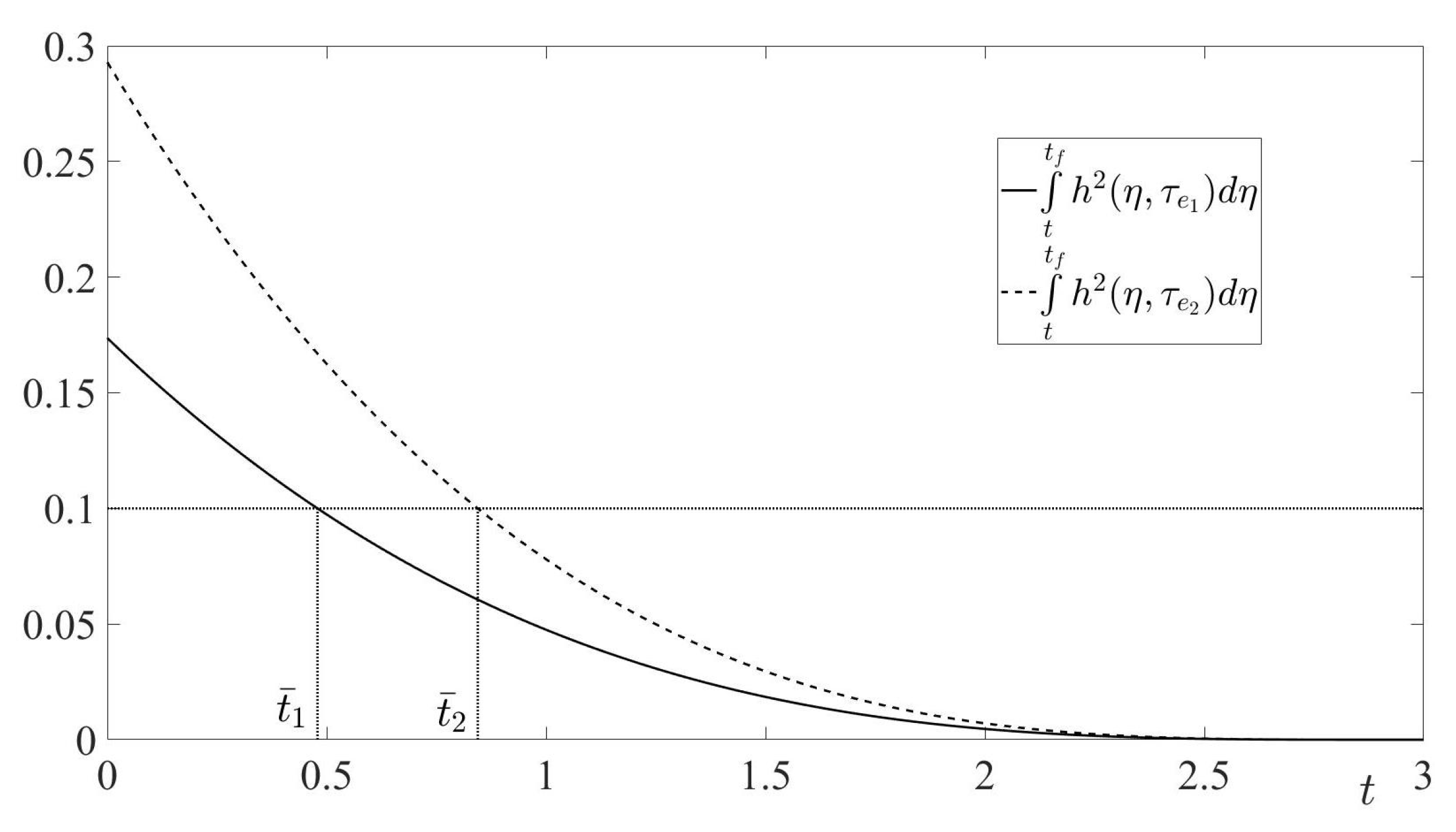
In this example, the moments, defined by (123), are s, s (see Figure 1).
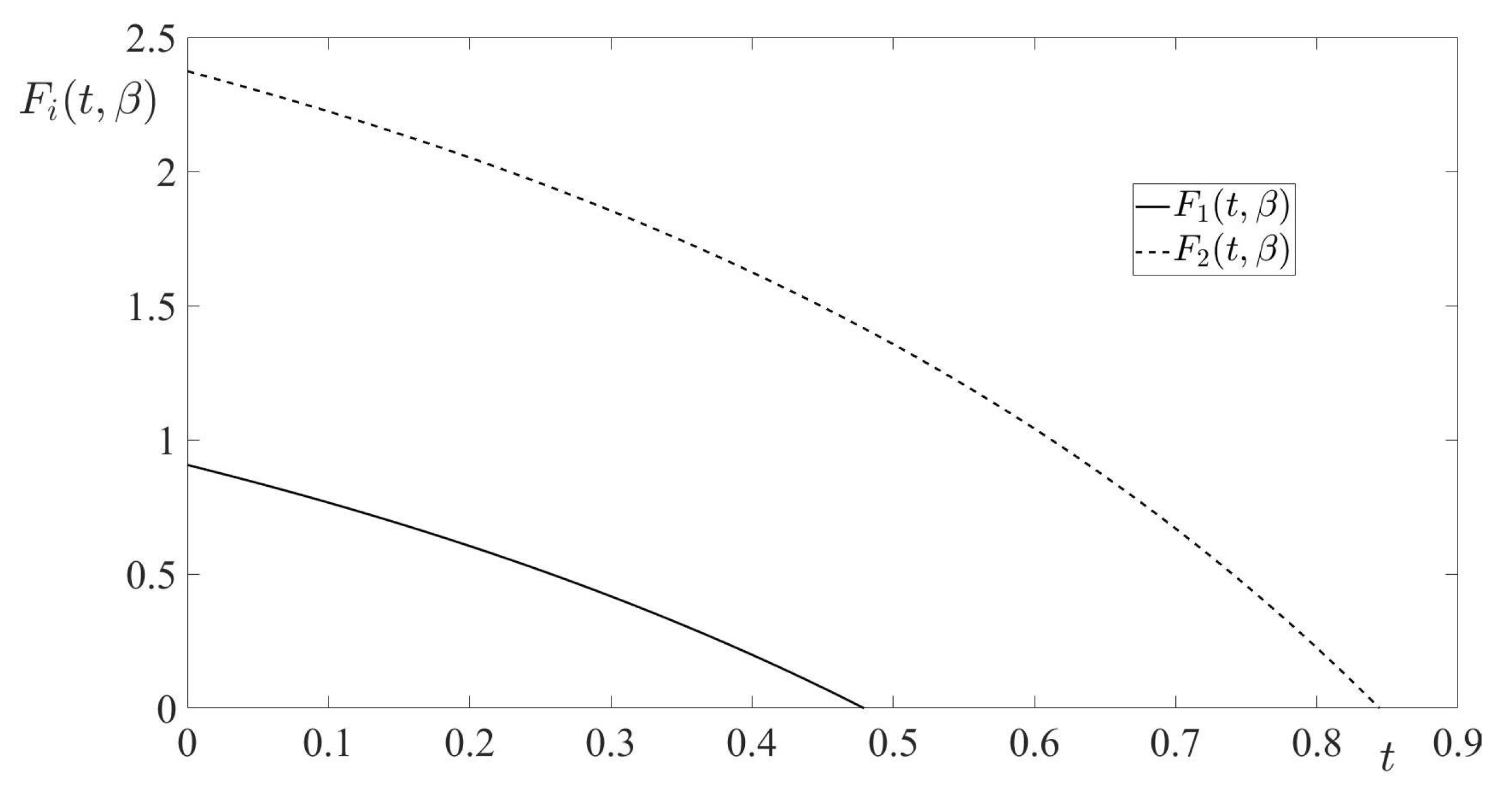
In Figure 2, the functions , given by (122), are shown for , . It is seen that these functions were decreasing. Therefore,
Due to (119) and (120), .
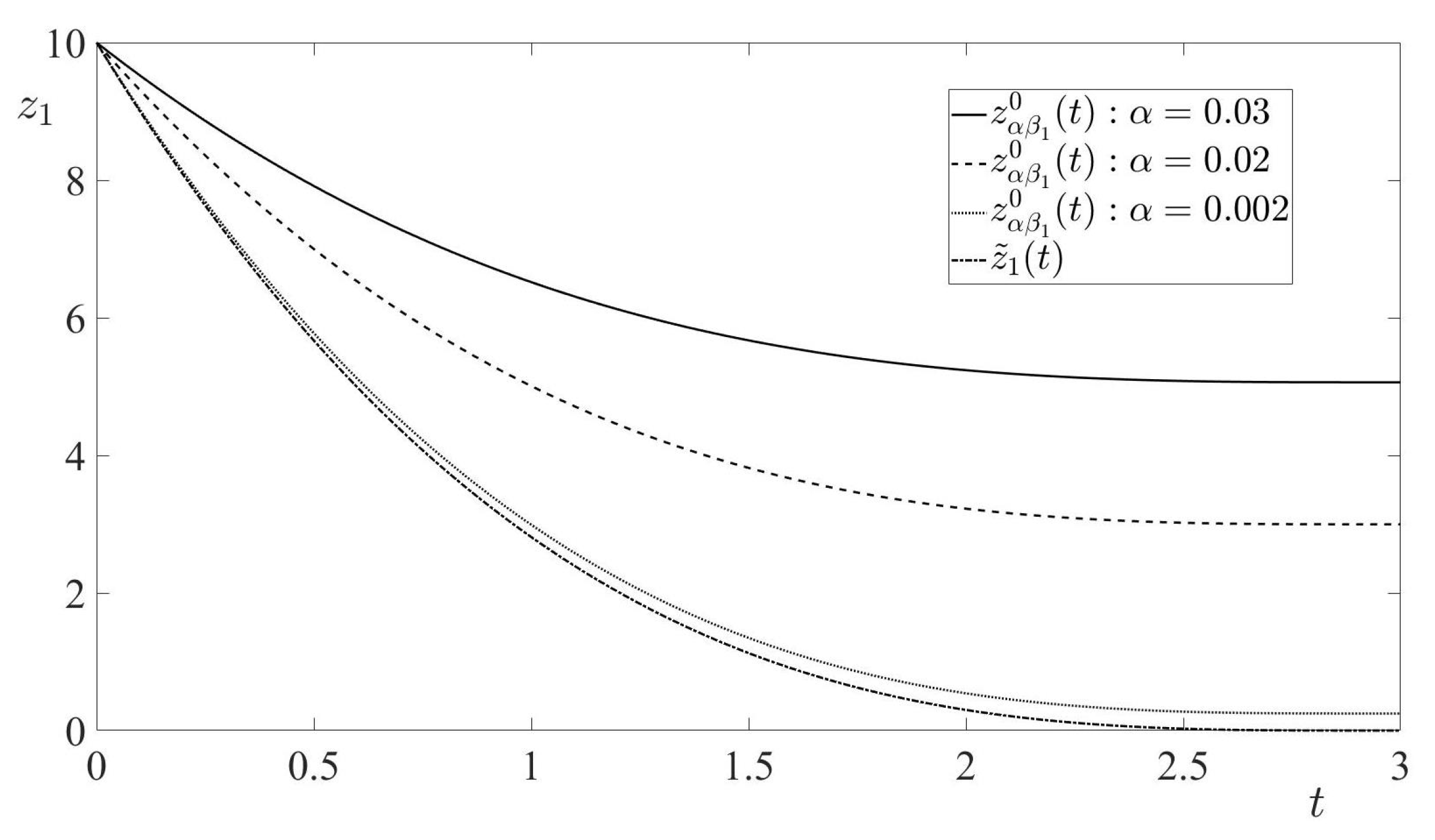
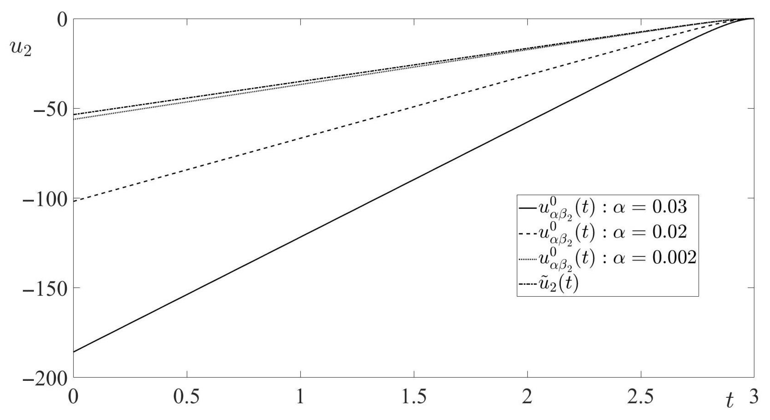
In Figure 3 and Figure 4, the components of the optimal trajectories are shown for decreasing values of , along with the components of the corresponding limiting function . It is clearly seen that the optimal trajectories tended to for , and tended to zero.
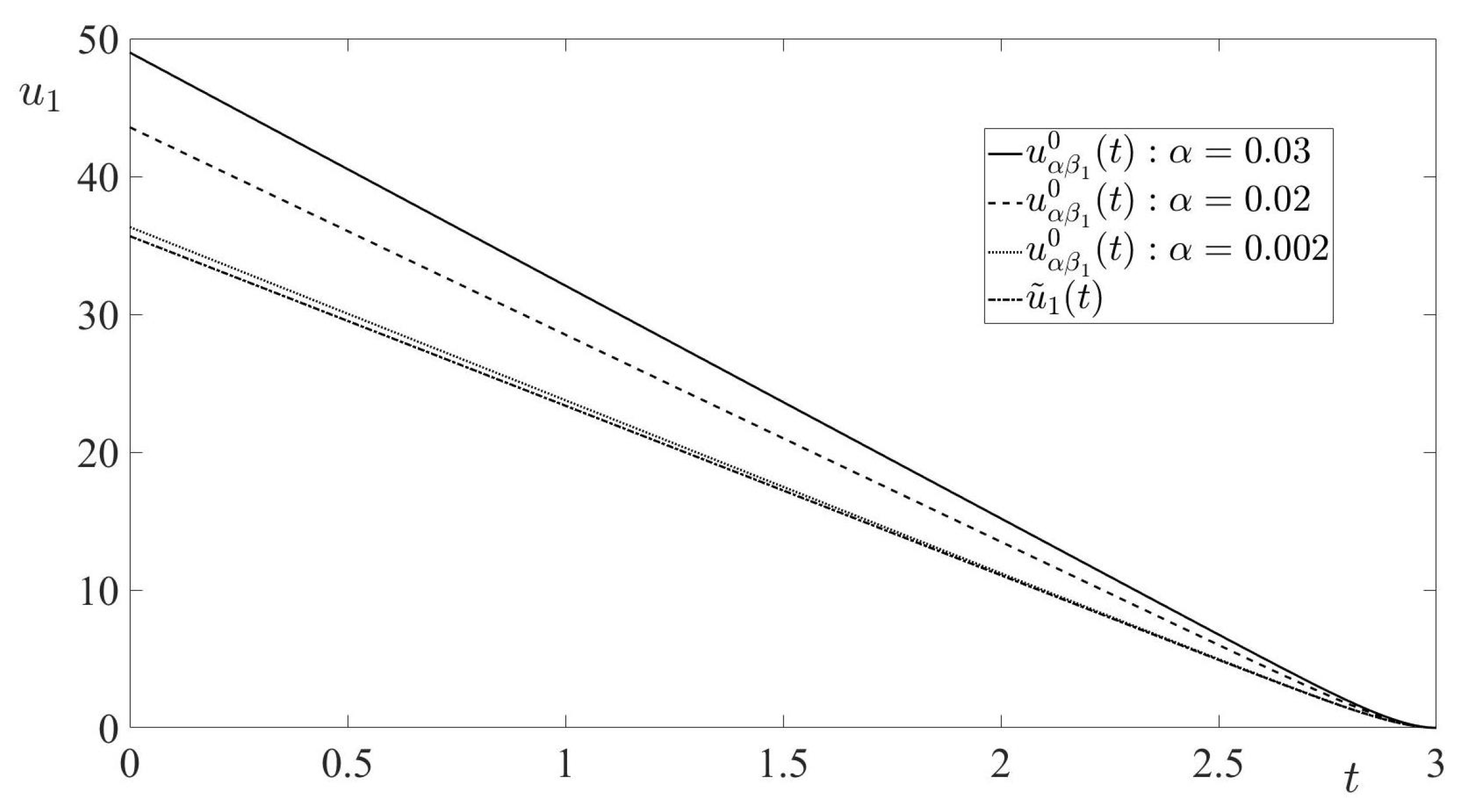
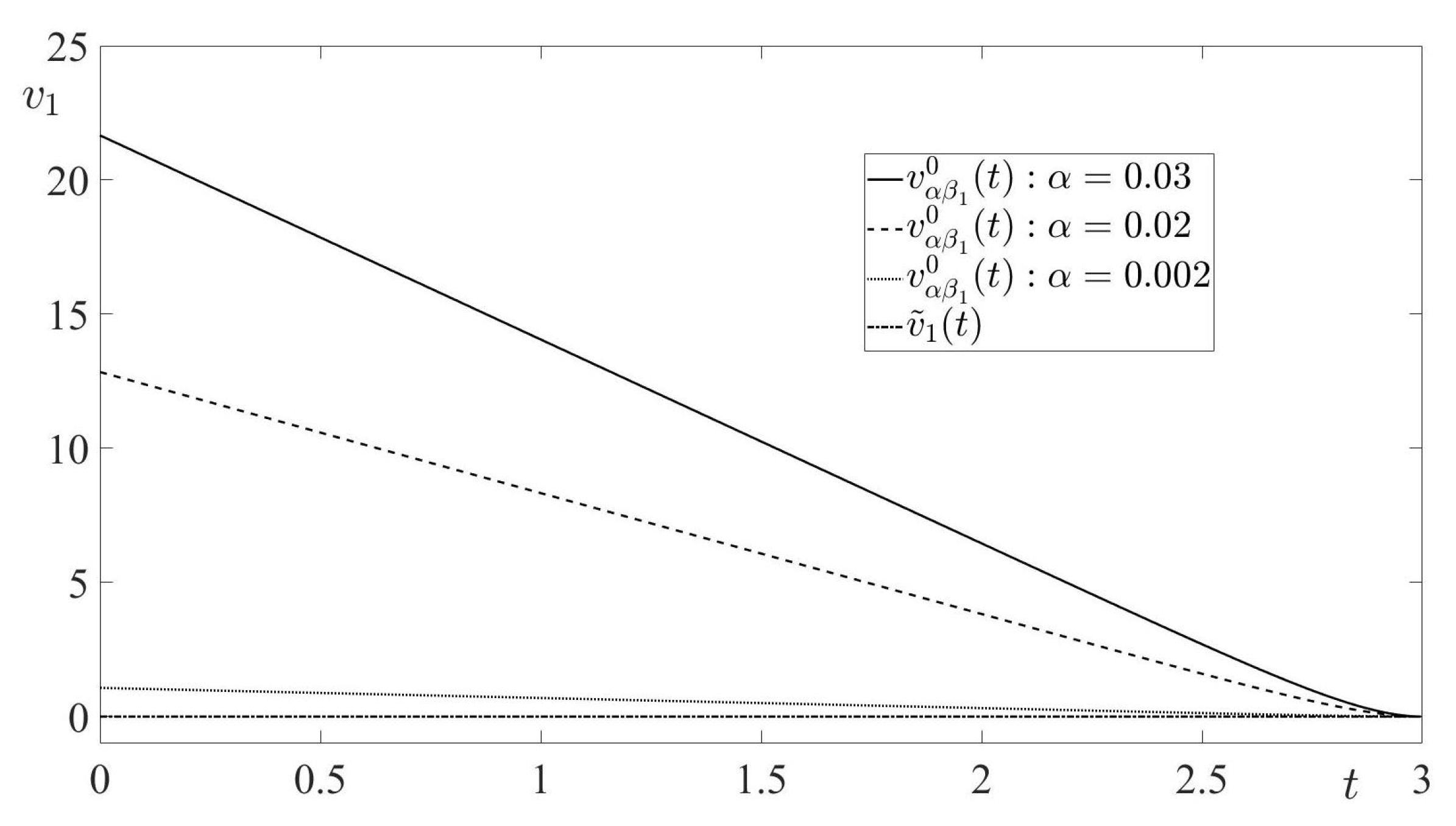
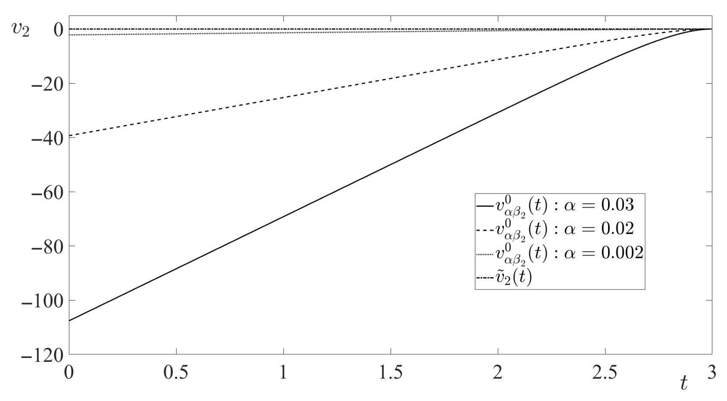
The respective components of time realizations of the optimal strategies and , along with the components of the corresponding limiting functions and , are depicted in Figure 5, Figure 6, Figure 7 and Figure 8, respectively. It is seen that the time realizations of the optimal strategies tended to the corresponding limiting functions for , remaining bounded.
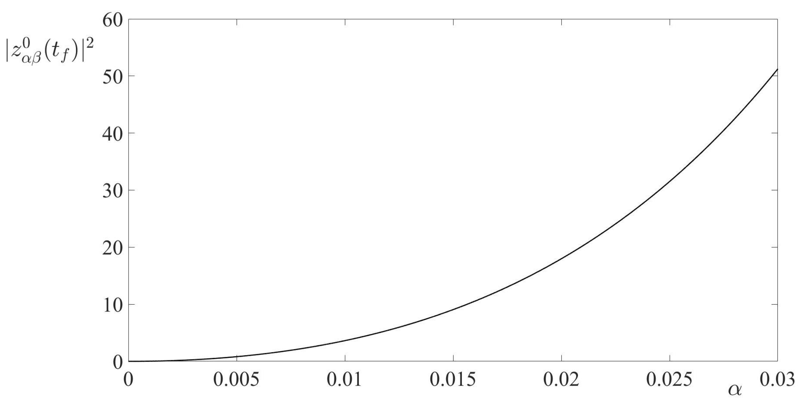
The game value is depicted in Figure 9 as a function of . It is seen that it tended to zero for .
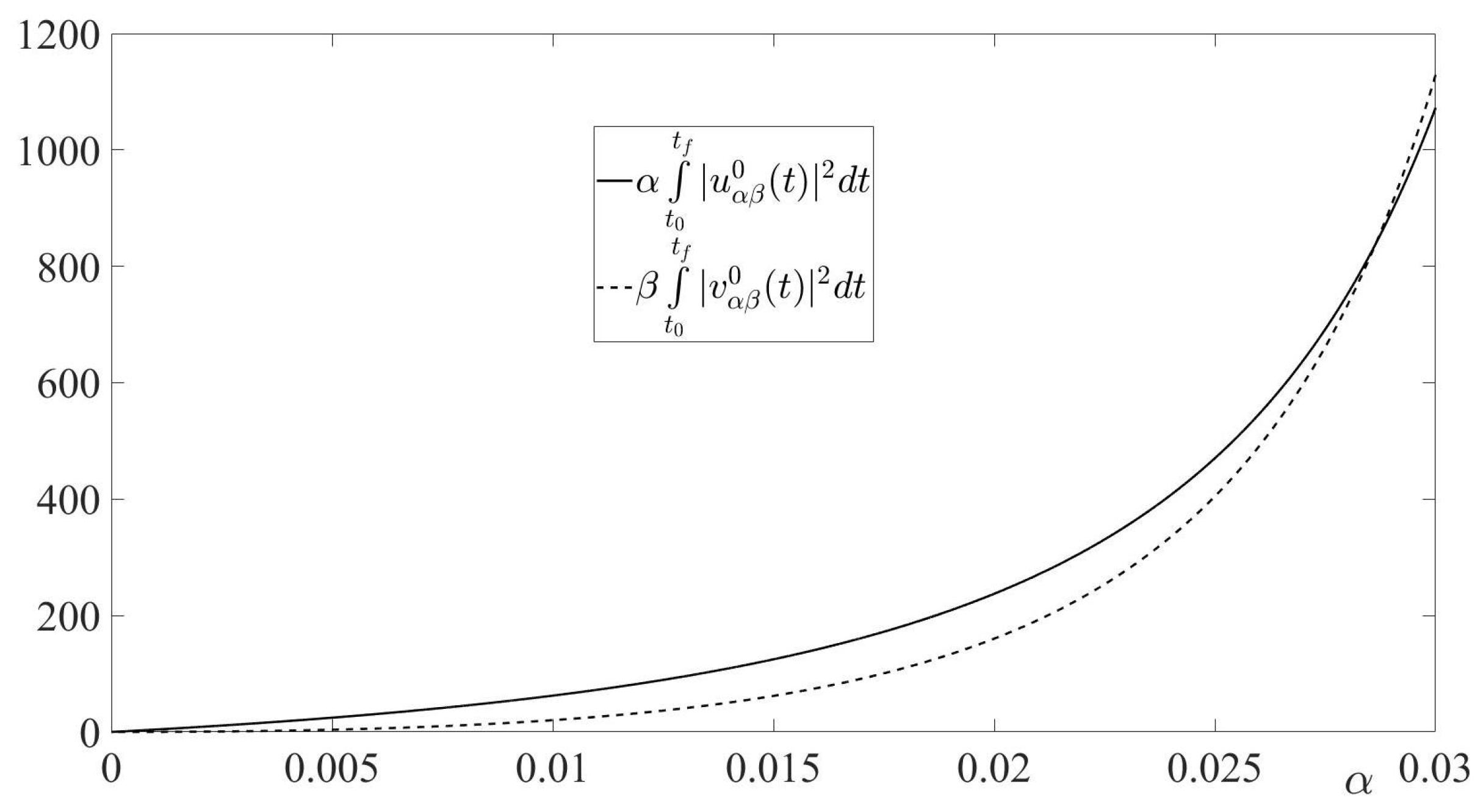
The respective terminal and integral terms of the cost function are shown in Figure 10 and Figure 11, respectively. It is seen that all components of the optimal cost tended to zero for .
Remark 10.
From Equation (125), it was seen that the small control cost of the interceptor yielded the high gain in its optimal state-feedback control. This important feature of the interceptor’s optimal state-feedback control increased considerably the ability of the interceptor to capture the target. One more important feature of the interceptor’s optimal state-feedback control was that the time realization of this control along the optimal interception’s trajectory and, especially, the trajectory itself, were bounded while the small parameter α tended to zero. Both aforementioned features of the interceptor’s state-feedback control, obtained by solution of the cheap control game, were extremely important in various real-life situations of a capture of a maneuverable flying target by a maneuverable flying interceptor. It should be noted that if the small control cost of the interceptor tended to zero, the ability of the interceptor to capture the target increased tending to the best achievable result, which was the zero-miss distance at the end of the interception.
6. Conclusions
In this paper, a pursuit-evasion problem, modeled by a finite-horizon linear-quadratic zero-sum differential game, was considered. In the game’s cost function, the penalty coefficient for the minimizing player’s control expenditure was a small value . Thus, the considered game was a zero-sum differential game with a cheap control of the minimizing player. By the proper state transformation, the initially formulated game was converted to a smaller Euclidean dimension differential game, called the reduced game. This game, also was a cheap control game and it was treated in the sequel of the paper. Due to the game’s solvability conditions, the solution of the reduced cheap control game was converted to the solution of the terminal-value problem for the matrix Riccati differential equation. Sufficient condition for the existence of the solution to this terminal-value problem in the entire interval of the game’s duration was presented, and the solution of this terminal-value problem was obtained. Using this solution, the value of the reduced cheap control game, as well as the optimal state-feedback controls of the minimizing player (the pursuer) and the maximizing player (the evader), were derived. The trajectory of the game, generated by the optimal players’ state-feedback controls, (the optimal trajectory), was obtained. The limits of the optimal trajectory, as well as of the time realizations of the players’ optimal state-feedback controls along the optimal trajectory, for were calculated. By this calculation, the boundedness of the optimal trajectory and the corresponding time realizations of the players’ optimal state-feedback controls for were shown. The limit of the game value for also was calculated, yielding the best achievable game value from the pursuer’s viewpoint. Along with the cheap control game, its degenerate version was considered. This version was obtained from the cheap control game by setting there formally , yielding the new zero-sum linear-quadratic pursuit-evasion game. This new game was singular, because it could not be solved either by the Isaacs’s MinMax principle or by the Bellman–Isaacs equation method. For this singular game, the notion of the pursuer’s minimizing sequence of state-feedback controls (instead of the pursuer’s optimal state-feedback control) was proposed. It was established that the -dependent pursuer’s optimal state-feedback control in the cheap control game constituted the pursuer’s minimizing sequence of state-feedback controls (as ) in the singular game. It was shown that the limit of this minimizing sequence was not an admissible pursuer’s state-feedback control in the singular game. However, the evader’s optimal state-feedback control and the value of the singular game coincided with the limits (for ) of the evader’s optimal state-feedback control and the value, respectively, of the cheap control game. Based on the theoretical results of the paper, the interception problem in 3D space, modeled by a zero-sum linear-quadratic game with the eight-dimensional dynamics, was studied. Similarly to the theoretical part of the paper, the case of the small penalty coefficient for the pursuer’s (interceptor’s) control expenditure in the cost function was considered. By proper linear state transformation, the original cheap control game was reduced to the new cheap control game with the two-dimensional dynamics. The asymptotic behaviour of the solution to this new game for was analyzed.
Author Contributions
The authors contributed equally to this article. All authors have read and agreed to the published version of the manuscript.
Funding
This research received no external funding.
Data Availability Statement
Not applicable.
Conflicts of Interest
The authors declare no conflict of interest.
References
- Bell, D.J.; Jacobson, D.H. Singular Optimal Control Problems; Academic Press: Cambridge, MA, USA, 1975. [Google Scholar]
- Kurina, G.A. A degenerate optimal control problem and singular perturbations. Soviet Math. Dokl. 1977, 18, 1452–1456. [Google Scholar]
- Glizer, V.Y. Stochastic singular optimal control problem with state delays: Regularization, singular perturbation, and minimizing sequence. SIAM J. Control Optim. 2012, 50, 2862–2888. [Google Scholar] [CrossRef]
- Shinar, J.; Glizer, V.Y.; Turetsky, V. Solution of a singular zero-sum linear-quadratic differential game by regularization. Int. Game Theory Rev. 2014, 16, 1–32. [Google Scholar] [CrossRef]
- Kwakernaak, H.; Sivan, R. The maximally achievable accuracy of linear optimal regulators and linear optimal filters. IEEE Trans. Autom. Control 1972, 17, 79–86. [Google Scholar] [CrossRef] [Green Version]
- Braslavsky, J.H.; Seron, M.M.; Mayne, D.Q.; Kokotović, P.V. Limiting performance of optimal linear filters. Automatica 1999, 35, 189–199. [Google Scholar] [CrossRef]
- Seron, M.M.; Braslavsky, J.H.; Kokotović, P.V.; Mayne, D.Q. Feedback limitations in nonlinear systems: From Bode integrals to cheap control. IEEE Trans. Autom. Control 1999, 44, 829–833. [Google Scholar] [CrossRef] [Green Version]
- Kokotović, P.V.; Khalil, H.K.; O’Reilly, J. Singular Perturbation Methods in Control: Analysis and Design; Academic Press: London, UK, 1986. [Google Scholar]
- Young, K.D.; Kokotović, P.V.; Utkin, V.I. A singular perturbation analysis of high-gain feedback systems. IEEE Trans. Autom. Control 1977, 22, 931–938. [Google Scholar] [CrossRef]
- Moylan, P.J.; Anderson, B.D.O. Nonlinear regulator theory and an inverse optimal control problem. IEEE Trans. Autom. Control 1973, 18, 460–465. [Google Scholar] [CrossRef]
- Turetsky, V.; Glizer, V.Y. Robust solution of a time-variable interception problem: A cheap control approach. Int. Game Theory Rev. 2007, 9, 637–655. [Google Scholar] [CrossRef]
- Turetsky, V.; Glizer, V.Y.; Shinar, J. Robust trajectory tracking: Differential game/cheap control approach. Int. J. Systems Sci. 2014, 45, 2260–2274. [Google Scholar] [CrossRef]
- Turetsky, V.; Shinar, J. Missile guidance laws based on pursuit—Evasion game formulations. Automatica 2003, 39, 607–618. [Google Scholar] [CrossRef]
- Turetsky, V. Upper bounds of the pursuer control based on a linear-quadratic differential game. J. Optim. Theory Appl. 2004, 121, 163–191. [Google Scholar] [CrossRef]
- Petersen, I.R. Linear-quadratic differential games with cheap control. Syst. Control Lett. 1986, 8, 181–188. [Google Scholar] [CrossRef]
- Glizer, V.Y. Asymptotic solution of zero-sum linear-quadratic differential game with cheap control for the minimizer. NoDEA Nonlinear Diff. Equ. Appl. 2000, 7, 231–258. [Google Scholar] [CrossRef]
- Vasil’eva, A.B.; Butuzov, V.F.; Kalachev, L.V. The Boundary Function Method for Singular Perturbation Problems; SIAM Books: Philadelphia, PA, USA, 1995. [Google Scholar]
- Bryson, A.; Ho, Y. Applied Optimal Control; Hemisphere: New York, NY, USA, 1975. [Google Scholar]
- Zhukovskii, V.I. Analytic design of optimum strategies in certain differential games. I. Autom. Remote Control 1970, 4, 533–536. [Google Scholar]
- Krasovskii, N.N.; Subbotin, A.I. Game-Theoretical Control Problems; Springer: New York, NY, USA, 1988. [Google Scholar]
- Basar, T.; Olsder, G.J. Dynamic Noncooperative Game Theory; Academic Press: London, UK, 1992. [Google Scholar]
- Petrosyan, L.A.; Zenkevich, N.A. Game Theory; World Scientific Publishing Company: Singapore, 2016. [Google Scholar]
- Isaacs, R. Differential Games; John Wiley: New York, NY, USA, 1965. [Google Scholar]
- Turetsky, V. Robust route realization by linear-quadratic tracking. J. Optim. Theory Appl. 2016, 170, 977–992. [Google Scholar] [CrossRef]
- Kalman, R.E. Contributions to the Theory of Optimal Control. Bol. Soc. Mat. Mex. 1960, 5, 102–119. [Google Scholar]
- Shinar, J.; Gutman, S. Three-Dimensional Optimal Pursuit and Evasion with Bounded Controls. IEEE Trans. Autom. Control 1980, 25, 492–496. [Google Scholar] [CrossRef]
- Shinar, J.; Medinah, M.; Biton, M. Singular surfaces in a linear pursuit-evasion game with elliptical vectograms. J. Optim. Theory Appl. 1984, 43, 431–458. [Google Scholar] [CrossRef]
Figure 1.
Moments .

Figure 2.
Functions .

Figure 3.
Trajectories and limiting function .

Figure 4.
Trajectories and limiting function .

Figure 5.
Time realizations and limiting function .

Figure 6.
Time realizations and limiting function .

Figure 7.
Time realizations and limiting function .

Figure 8.
Time realizations and limiting function .

Figure 9.
The game value.

Figure 10.
The terminal term of the cost function.

Figure 11.
Integral terms of the cost function.

Publisher’s Note: MDPI stays neutral with regard to jurisdictional claims in published maps and institutional affiliations. |
© 2022 by the authors. Licensee MDPI, Basel, Switzerland. This article is an open access article distributed under the terms and conditions of the Creative Commons Attribution (CC BY) license (https://creativecommons.org/licenses/by/4.0/).
Share and Cite
MDPI and ACS Style
Turetsky, V.; Glizer, V.Y. Cheap Control in a Non-Scalarizable Linear-Quadratic Pursuit-Evasion Game: Asymptotic Analysis. Axioms 2022, 11, 214. https://0-doi-org.brum.beds.ac.uk/10.3390/axioms11050214
AMA Style
Turetsky V, Glizer VY. Cheap Control in a Non-Scalarizable Linear-Quadratic Pursuit-Evasion Game: Asymptotic Analysis. Axioms. 2022; 11(5):214. https://0-doi-org.brum.beds.ac.uk/10.3390/axioms11050214
Chicago/Turabian StyleTuretsky, Vladimir, and Valery Y. Glizer. 2022. "Cheap Control in a Non-Scalarizable Linear-Quadratic Pursuit-Evasion Game: Asymptotic Analysis" Axioms 11, no. 5: 214. https://0-doi-org.brum.beds.ac.uk/10.3390/axioms11050214
Note that from the first issue of 2016, this journal uses article numbers instead of page numbers. See further details here.