A Symplectic Algorithm for Constrained Hamiltonian Systems

Abstract

In this paper, a symplectic algorithm is utilized to investigate constrained Hamiltonian systems. However, the symplectic method cannot be applied directly to the constrained Hamiltonian equations due to the non-canonicity. We firstly discuss the canonicalization method of the constrained Hamiltonian systems. The symplectic method is used to constrain Hamiltonian systems on the basis of the canonicalization, and then the numerical simulation of the system is carried out. An example is presented to illustrate the application of the results. By using the symplectic method of constrained Hamiltonian systems, one can solve the singular dynamic problems of nonconservative constrained mechanical systems, nonholonomic constrained mechanical systems as well as physical problems in quantum dynamics, and also available in many electromechanical coupled systems.

1. Introduction

In 1993, symplectic algorithms for constrained Hamiltonian systems have been proposed [1]. We know that the displacements q and momenta p of an object moving freely are given by a Hamilton canonical equation in the form [2]

$$\dot{q}={\nabla }_{p}H(p, q), \dot{p}=-{\nabla }_q\left(p,q\right)$$

(1)

where $p, q\in R^n$, $H:{ R}^n\times R^n\to { R}^n$ is called the Hamiltonian function. A natural question is what happens when (1) is constrained by algebraic equations on q and/or p. That is, there are Hamiltonian constraints of the form $g\left(q\right)=0$, and it leads to the constraints of Hamiltonian equations as [3,4]

$$\dot{q}={\nabla }_{p}H(p, q), \dot{p}=-{\nabla }_{q}H\left(p,q\right)-\mathsf{\lambda }G{\left(q\right)}^t,$$

(2)

where $g:{ R}^n\to { R}^n$, $G\left(q\right)=g_q\left(q\right)\in R^{n\times m}$ and $\mathsf{\lambda }\in R^m$. Equation (2) is called a constrained Hamiltonian system, which is not only a relatively loose concept but also a general constrained mechanical system. The flow of a Hamiltonian system like (1) possesses an important symplectic geometric structure. It has been observed in numerical experiments that symplectic methods with fixed step-size possess better long-term stability properties. Leimkuhler and Skeel [5] investigated symplectic numerical integrators of constrained Hamiltonian systems in molecular dynamics. By composition methods, Reich [6] studied symplectic integration of the constrained Hamiltonian systems. The method they proposed can reduce Hamiltonian differential-algebraic equations to ordinary differential equations in Euclidean space.

When studying symmetry properties of classical and quantum constrained systems, Li [7,8] found that via Legendre transformation, a singular Lagrangian system can be transformed into the phase space determined by generalized momenta and generalized coordinates. Since there are inherent constraints between generalized momenta and generalized coordinates, it is named a constrained Hamiltonian system. A lot of important physical systems belong to this system, such as quantum electrodynamics, quantum flavor dynamics, and so on. Even many electromechanical coupled systems belong to constrained Hamiltonian systems. For a Lagrangian system, if the value of determinant $\det \left(\frac{{\partial }^{2}L}{\partial q_s\partial q_k}\right)$ vanishes, then it is named as a singular Lagrange system. The Lagrangian function of supersymmetry, supergravity, and string theory are all singular. Therefore, the fundamental theory of constrained Hamiltonian systems acts an important role in modern quantum field theory [9].

In the late 1980s, Feng et al. established the so-called symplectic algorithms to study the equations in Hamiltonian form and showed that these methods are more superior over a long time by combining theoretical analysis and computer experimentation [10,11]. The symplectic method has been widely recognized as a suitable numerical integrator with global conservation properties for canonical Hamiltonian systems. It has been well applied in testing particle simulation and some physical experiments in plasma physics, and thus derived a series of results, for instance, a variational multi-symplectic particle-in-cell algorithm of the Vlasov-Maxwell system [12], the practical symplectic partitioned Runge-Kutta and Runge-Kutta-Nystrom methods [13], the symplectic integrations of Hamiltonian systems [14], symplectic integrators of the Ablowitz–Ladik discrete nonlinear Schrödinger equation [15], etc. The standard symplectic scheme normally works for a canonical structure of the dynamical system. However, the symplectic simulation for the constrained Hamiltonian systems is beset with difficulties since the constrained Hamiltonian systems are usually non-canonical.

In this paper, we will present a general procedure for constructing the canonical coordinates of constrained Hamiltonian systems. By defining a variable transformation and calculations, the canonical variables for constrained Hamiltonian systems can be derived, and thus the constrained Hamiltonian systems are canonicalized. Once the canonical coordinates of constrained Hamiltonian systems are derived, one can employ the standard canonical symplectic methods to study the constrained Hamiltonian systems. The method we proposed is of importance in the study of constrained Hamiltonian systems. We believe that the symplectic method of constrained Hamiltonian systems given in this paper can be used in the study of quantum dynamics, electromechanical coupled systems, and strange constrained dynamics as well.

To verify the effect of the canonicalization and illustrate the advantage of the canonical symplectic simulation, a numerical example of the constrained Hamiltonian system is presented. Clearly, the numerical results derived by the canonical symplectic method are more accurate in the long-term simulation since they can maintain conservation properties.

2. Canonicalization of Constrained Hamiltonian Systems

Assume that a mechanical system is determined by the generalized coordinates $q_i(i=1,2,\dots ,n)$, and the Lagrangian function $L=L(t,q_i,{\dot{q}}_i)$ satisfies $\det \left(\frac{{\partial }^{2}L}{\partial q_s\partial q_k}\right)=0$ When the generalized momenta and Hamiltonian of the system are constructed, there are inherent constraints between the canonical variables in the phase space

$${\varphi }_j(t,q_i,p_i)=0\begin{array}{cc}& (j=1,2,\dots ,n-r,i=j=1,2,\dots ,n)\end{array}$$

(3)

this is the constraint equation that should be obtained between the generalized coordinates and the generalized momenta of the constrained Hamiltonian system.

Then the motion equations of a singular system can be written as [11]

$${\dot{q}}_i=\frac{\partial H_c}{\partial p_i}+{\lambda }_j\frac{\partial {\phi }_j}{\partial p_i},\begin{array}{cc}& {\dot{p}}_i=-\frac{\partial H_c}{\partial q_i}-{\lambda }_j\frac{\partial {\phi }_j}{\partial q_i}\end{array}\begin{array}{cc}& (i=1,2,\dots ,n)\end{array}$$

(4)

where $H_c$ is the Hamiltonian of the system and ${\lambda }_j$ is the Lagrange multiplier. The multiplier in Formula (4) can be given by Equations (3) and (4).

The motion Equation (4) of the constrained Hamiltonian system can be rewritten as

$$\left(\begin{array}{c}{\dot{p}}_1\\ ⋮\\ {\dot{p}}_i\\ {\dot{q}}_1\\ ⋮\\ {\dot{q}}_n\end{array}\right)=\left(\begin{array}{cc}{0}_n& S_n\\ T_n& 0_n\end{array}\right)\left(\begin{array}{c}\frac{\partial H_c}{\partial p_1}\\ ⋮\\ \frac{\partial H_c}{\partial p_i}\\ \frac{\partial H_c}{\partial q_1}\\ ⋮\\ \frac{\partial H_c}{\partial q_i}\end{array}\right)=M_{2n\times 2n}\left(\begin{array}{c}\frac{\partial H_c}{\partial p_1}\\ ⋮\\ \frac{\partial H_c}{\partial p_i}\\ \frac{\partial H_c}{\partial q_1}\\ ⋮\\ \frac{\partial H_c}{\partial q_i}\end{array}\right),$$

(5)

where

$$S_n={\left(\begin{array}{ccc}-1-{\lambda }_j\frac{\partial {\phi }_j}{\partial H_c}& \dots & 0\\ ⋮& \ddots & ⋮\\ 0& \cdots & -1-{\lambda }_j\frac{\partial {\phi }_j}{\partial H_c}\end{array}\right)}_{n\times n},T_n={\left(\begin{array}{ccc}1+{\lambda }_j\frac{\partial {\phi }_j}{\partial H_c}& \dots & 0\\ ⋮& \ddots & ⋮\\ 0& \cdots & 1+{\lambda }_j\frac{\partial {\phi }_j}{\partial H_c}\end{array}\right)}_{n\times n}$$

(6)

and $M_{2n\times 2n}$ is an anti-symmetric matrix.

Let $v={(p,q)}^T$, where $\begin{array}{cc}p=(p_1,p_2,\dots ,p_n),& q=(q_1,q_2,\dots ,q_n)\end{array},$ then Equation (5) can be rewritten as

$$\dot{v}=K{(v)}^{-1}\nabla H_c(v),$$

(7)

where

$$K(v)=\left(\begin{array}{cc}{0}_n& T_n^{-1}\\ S_n^{-1}& 0_n\end{array}\right).$$

(8)

It is easy to see that Equations (5) and (7) are non-canonical Hamiltonian systems.

To rewrite the non-canonical Hamiltonian system in canonical form, we let $Z=\Psi (v)$ be the corresponding canonical variables which is a transformation from $R^{2n}$ to $R^{2n}$. $Z={(\tilde{p},\tilde{q})}^T$ are new variables after canonicalization. By the chain rule, the canonicalization of Equation (7) can be written as [11]

$$\dot{Z}=\left(\frac{\partial \Psi }{\partial v}\right)K{(v)}^{-1}{\left(\frac{\partial \Psi }{\partial v}\right)}^T\nabla \tilde{H}(Z),$$

(9)

where $\tilde{H}(Z)=H_c(v)$. If we let $\left(\frac{\partial \Psi }{\partial v}\right)K{(v)}^{-1}{\left(\frac{\partial \Psi }{\partial v}\right)}^T=J^{-1},$ i.e.,

$$K(v)={\left(\frac{\partial \Psi }{\partial v}\right)}^{T}J\left(\frac{\partial \Psi }{\partial v}\right)$$

(10)

Note that $K(v)$ is a given matrix and $v={(p,q)}^T$ is the original variable, so we can get $\Psi (v)$ through this transformation, which is a set of canonical new generalized momenta $\tilde{p}=({\tilde{p}}_1,{\tilde{p}}_2,\dots ,{\tilde{p}}_n)$ and generalized coordinates $\tilde{q}=({\tilde{q}}_1,{\tilde{q}}_2,\dots ,{\tilde{q}}_n)$. Now, we have transformed the non-canonical Hamiltonian system into a canonical Hamiltonian system.

By substituting the new variables into the original Hamiltonian of the constrained system, it becomes canonical. Based on the canonical Hamiltonian equations, one can examine their properties and hence some useful algorithms can be applied to examine the numerical solutions and numerical simulation of the constrained Hamilton systems. The results of the original system can be obtained by replacing the new variables with the old ones.

3. Symplectic Method for Constrained Hamiltonian Systems

The constrained Hamiltonian systems are transformed in the canonical form (9):

$$\frac{dZ}{dt}=J^{-1}\tilde{\nabla }H(Z),$$

(11)

that is, the canonical Hamiltonian system is

$$\begin{array}{ccc}\frac{dZ}{dt}=J^{-1}\tilde{\nabla }H(Z),& J=\left(\begin{array}{cc}0& I_n\\ -I_n& 0\end{array}\right),& Z\in R^{2n}\end{array}$$

(12)

We now show that the properties, conclusions, and calculation methods of canonical Hamiltonian systems can be extended to constrained Hamiltonian systems. We give the symplectic method for constrained Hamiltonian systems as follows.

A transformation of the constrained Hamiltonian system

$$\begin{array}{cc}\Psi :R^{2n}\to R^{2n},& v=\left(\begin{array}{c}p\\ q\end{array}\right)\end{array}\to \tilde{Z}=\left(\begin{array}{c}\tilde{p}\\ \tilde{q}\end{array}\right)$$

(13)

is called the symplectic transformation for a system if its Jacobian is a symplectic matrix

$${\left(\frac{d\tilde{Z}}{dZ}\right)}^{T}J\left(\frac{d\tilde{Z}}{dZ}\right)=J\iff {\displaystyle \sum _{k=1}^{n}d{\tilde{p}}_k\wedge d{\tilde{q}}_k={\displaystyle \sum _{k=1}^{n}d{p}_k\wedge d{q}_k}}.$$

(14)

For the canonical Hamiltonian system (9), if

$$\begin{array}{cc}\tilde{p}=p-\tau \frac{\partial H}{\partial q}(\tilde{p},q),& \tilde{q}=q+\tau \frac{\partial H}{\partial p}(\tilde{p},q),\end{array}$$

(15)

then it is a first-order symplectic scheme. When $H(p,q)=U(p)+V(q)$, Equation (15) becomes

$$\begin{array}{cc}\tilde{p}=p-\tau \frac{\partial V}{\partial q}(q),& \tilde{q}=q+\tau \frac{\partial U}{\partial p}(\tilde{p}),\end{array}$$

(16)

which is an explicit symplectic scheme. For the canonical Hamiltonian system (9), the Euler midpoint rule is

$$\tilde{Z}=Z+\tau J^{-1}\nabla H(\frac{\tilde{Z}+Z}{2}),$$

(17)

which is a second-order symplectic scheme. A Runge-Kutta method

$$\begin{array}{cc}\tilde{Z}=Z+\tau {\displaystyle \sum _{i=1}^m{b}_i}{J}^{-1}\nabla H(K_i),& K_i=Z+\tau {\displaystyle \sum _{i=1}^m{a}_{ij}}{J}^{-1}\nabla H(K_j),\end{array}i=1,\dots ,m,$$

(18)

is symplectic if and only if $b_i{b}_j-b_i{a}_{ij}-b_j{a}_{ij}=0$. In Equations (15)–(18), τ represents the time step size.

4. Example

The Lotka-Volterra model can be expressed as a non-canonical Hamiltonian system with $n=1$

$$\left(\begin{array}{c}\dot{p}\\ \dot{q}\end{array}\right)=\left(\begin{array}{cc}0& -pq\\ pq& 0\end{array}\right)\nabla H(p,q),$$

(19)

where $H(p,q)=p-2\log p+q-\log q.$

The Hamiltonian $H$ can be rewritten as $H=H_1+H_2$ with $H_1=p-2\log p$ and $H_2=q-\log q.$ According to the canonialization method shown in Section 2, we have

$$K=\left(\begin{array}{cc}0& \frac{1}{pq}\\ -\frac{1}{pq}& 0\end{array}\right).$$

(20)

According to Equation (10), we get

$$\begin{array}{cc}\frac{\partial \tilde{p}}{\partial p}\frac{\partial \tilde{q}}{\partial p}-\frac{\partial \tilde{p}}{\partial p}\frac{\partial \tilde{q}}{\partial p}=0,& \frac{\partial \tilde{p}}{\partial p}\frac{\partial \tilde{q}}{\partial q}-\frac{\partial \tilde{q}}{\partial p}\frac{\partial \tilde{p}}{\partial q}=\end{array}\frac{1}{pq}$$

(21)

and

$$\begin{array}{cc}\tilde{p}=\log (p),& \tilde{q}=\log (q).\end{array}$$

(22)

Hence, we have

$$p=\exp (\begin{array}{cc}\tilde{p}),& q=\exp (\tilde{q})\end{array}$$

(23)

and thus

$$\tilde{H}(\tilde{p},\tilde{q})=\exp (\tilde{p})-2\tilde{p}+\exp (\tilde{q})-\tilde{q},$$

(24)

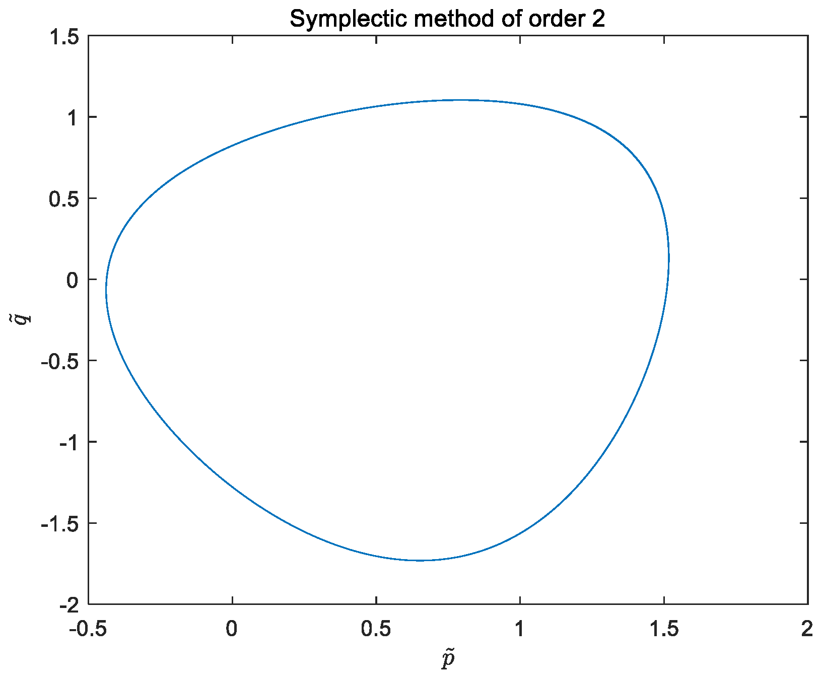
which is a canonical Hamiltonian system. Using the second-order explicit symplectic scheme on the basis of the canonicalization, we get the trajectory of the canonical variable $\begin{array}{cc}\tilde{p},& \tilde{q}\end{array}$, where $\tilde{p}\left(0\right)=\ln 2,$ $\tilde{q}\left(0\right)=\ln 3,$ and time step size $\tau =0.1$ (see Figure 1).

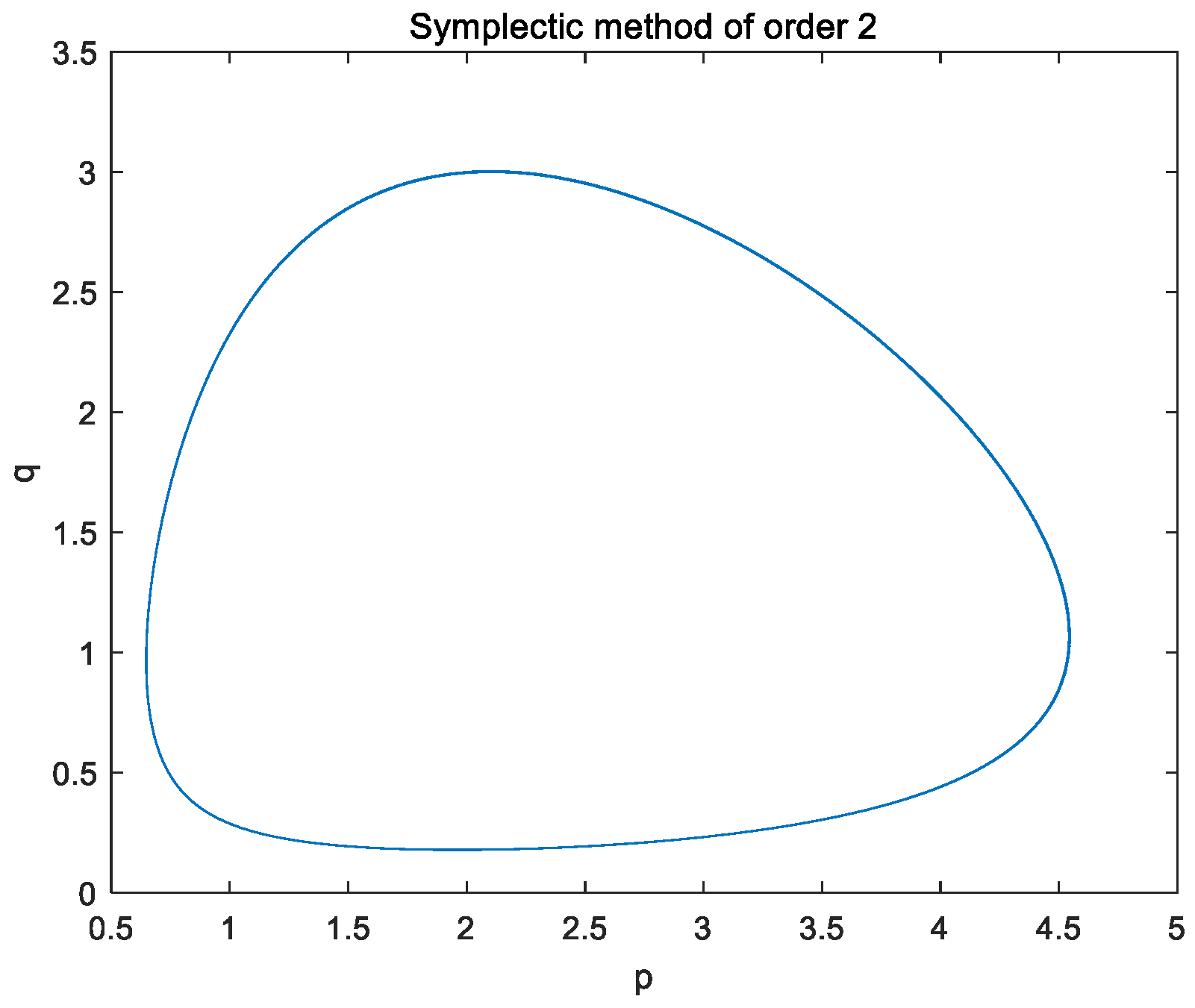
Using Equation (23) we can obtain $p,q,$ and $p\left(0\right)=2,$ $q\left(0\right)=3$, and time step size $\tau =0.1$, then using the second-order explicit symplectic scheme on the basis of $p,q$, we get the trajectory of the non-canonical variable $p,q$ (see Figure 2).

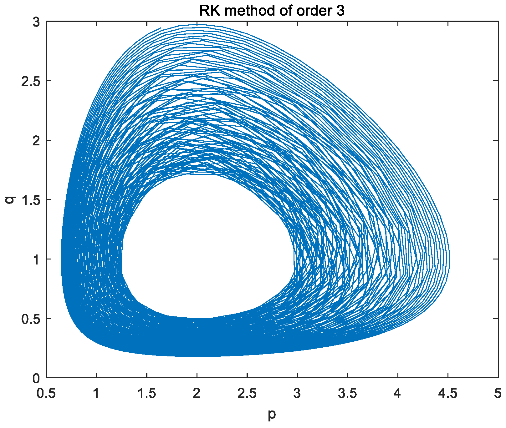
In addition, the implicit Runge-Kutta method of order 3 is applied directly to the non-canonical Hamiltonian system directly, and then we get the trajectory of the original variables $p,q$, and $p\left(0\right)=2,$ $q\left(0\right)=3$ and time step size $\tau =0.1$ (see Figure 3).

As can be seen from Figure 1 and Figure 2, the trajectory diagrams of regularized variables and initial variables are kept unchanged by a symplectic algorithm. After 1,000,000 steps, the graph remains basically unchanged, which indicates that the symplectic algorithm of constrained Hamiltonian systems has the property of preserving structure. Namely, the physical properties of constrained Hamiltonian systems can be maintained by a symplectic method. One can see from Figure 3 that the graph using the third-order Runge Kutta method (or general numerical calculation method) is very unstable. This method does not have the property of preserving the structure, that is, it cannot maintain the physical properties of the constrained Hamiltonian systems. It is shown clearly from the three figures that the symplectic algorithm has better structure-preserving properties. It is of great significance to study the constrained Hamiltonian systems using the symplectic algorithm.

5. Conclusions

In this paper, we discuss the canonicalization method of the constrained Hamiltonian systems, then the symplectic method is applied to the constrained Hamiltonian systems on the basis of the canonicalization. Compared with the traditional Runge-Kutta method, they have better structural preservation properties. Consequently, the symplectic methods can be applied to more noncanonical Hamiltonian systems, which will be further investigated in our next work.

References

- Reich, S. Symplectic Integration of Constrained Hamiltonian Systems by Runge-Kutta Methods; Technical Report 93-13; Department of Computer Science, University of British Columbia: Vancouver, BC, Canada, 1993. [Google Scholar]
- Hildebrand, F.B. Methods of Applied Mathematics, 2nd ed.; Prentice-Hall: Englewood Cliffs, NJ, USA, 1965. [Google Scholar]
- Dirac, P.A.M. Lecture on Quantum Mechanics; Yeshiva University Press: New York, NY, USA, 1964. [Google Scholar]
- Arnold, V.I. Mathematical Methods of Classical Mechanics, Graduate Texts in Mathematics, No. 60; Springer: New York, NY, USA, 1975. [Google Scholar]
- Leimkuhler, B.J.; Skeel, R.D. Symplectic numerical integrators in constrained Hamiltonian systems. J. Comput. Phys. 1994, 112, 117–125. [Google Scholar] [CrossRef] [Green Version]
- Reich, S. Symplectic Integration of Constrained Hamiltonian Systems by Composition Methods. SIAM J. Numer. Anal. 1996, 33, 475–491. [Google Scholar] [CrossRef] [Green Version]
- Li, Z.P. Classical and Quantal Dynamics of Constrained System and Their Symmetrical Properties; Beijing Polytechnic Univ. Press: Beijing, China, 1993. [Google Scholar]
- Li, Z.P.; Jiang, J.H. Symmetries in Constrained Canonical System; Beijing Science Press: Beijing, China, 2002. [Google Scholar]
- Holod, I.; Lin, Z. Verification of electromagnetic fluid-kinetic hybrid electron model in global Gyrokinetic particle simulation. Phys. Plasmas 2013, 20, 032309. [Google Scholar] [CrossRef] [Green Version]
- Feng, K.; Qin, M. Symplectic Geometric Algorithms for Hamiltonian Systems; Zhejiang Science and Technology Publishing House: Hangzhou, China, 2010. [Google Scholar]
- Feng, K.; Qin, M. Symplectic difference schemes for Hamiltonian systems. J. Comp. Math. 1991, 1, 86–96. [Google Scholar]
- Xiao, J.; Liu, J.; Qin, H. A variational multi-symplectic particle-in-cell algorithm with smoothing functions for the Vlasov-Maxwell system. Phys. Plasmas 2013, 20, 102517. [Google Scholar] [CrossRef]
- Blanes, S.; Moan, P.C. Practical symplectic partitioned Runge-Kutta and Runge-Kutta-Nystrom methods. J. Comp. Appl. Math. 2000, 142, 313–330. [Google Scholar] [CrossRef] [Green Version]
- Channell, P.J.; Scovel, C. Symplectic integration of Hamiltonian systems. Nonlinearity 1990, 3, 231–259. [Google Scholar] [CrossRef]
- Schober, C.M. Symplectic integrators for the Ablowitz–Ladik discrete nonlinear Schrödinger equation. Phys. Lett. A 1999, 259, 140–151. [Google Scholar] [CrossRef]
Figure 1.
Trajectory of the canonical variable .
Figure 2.
Trajectory of the non-canonical variable .
Figure 3.
Trajectory of the non-canonical variable.
Publisher’s Note: MDPI stays neutral with regard to jurisdictional claims in published maps and institutional affiliations. |
© 2022 by the authors. Licensee MDPI, Basel, Switzerland. This article is an open access article distributed under the terms and conditions of the Creative Commons Attribution (CC BY) license (https://creativecommons.org/licenses/by/4.0/).
Share and Cite
MDPI and ACS Style
Fu, J.; Zhang, L.; Cao, S.; Xiang, C.; Zao, W. A Symplectic Algorithm for Constrained Hamiltonian Systems. Axioms 2022, 11, 217. https://0-doi-org.brum.beds.ac.uk/10.3390/axioms11050217
AMA Style
Fu J, Zhang L, Cao S, Xiang C, Zao W. A Symplectic Algorithm for Constrained Hamiltonian Systems. Axioms. 2022; 11(5):217. https://0-doi-org.brum.beds.ac.uk/10.3390/axioms11050217
Chicago/Turabian StyleFu, Jingli, Lijun Zhang, Shan Cao, Chun Xiang, and Weijia Zao. 2022. "A Symplectic Algorithm for Constrained Hamiltonian Systems" Axioms 11, no. 5: 217. https://0-doi-org.brum.beds.ac.uk/10.3390/axioms11050217
Note that from the first issue of 2016, this journal uses article numbers instead of page numbers. See further details here.