New Fuzzy Extensions on Binomial Distribution

Abstract

The use of discrete probabilistic distributions is relevant to many practical tasks, especially in present-day situations where the data on distribution are insufficient and expert knowledge and evaluations are the only instruments for the restoration of probability distributions. However, in such cases, uncertainty arises, and it becomes necessary to build suitable approaches to overcome it. In this direction, this paper discusses a new approach of fuzzy binomial distributions (BDs) and their extensions. Four cases are considered: (1) When the elementary events are fuzzy. Based on this information, the probabilistic distribution of the corresponding fuzzy-random binomial variable is calculated. The conditions of restrictions on this distribution are obtained, and it is shown that these conditions depend on the ratio of success and failure of membership levels. The formulas for the generating function (GF) of the constructed distribution and the first and second order moments are also obtained. The Poisson distribution is calculated as the limit case of a fuzzy-random binomial experiment. (2) When the number of successes is of a fuzzy nature and is represented as a fuzzy subset of the set of possible success numbers. The formula for calculating the probability of convolution of binomial dependent fuzzy events is obtained, and the corresponding GF is built. As a result, the scheme for calculating the mathematical expectation of the number of fuzzy successes is defined. (3) When the spectrum of the extended distribution is fuzzy. The discussion is based on the concepts of a fuzzy-random event and its probability, as well as the notion of fuzzy random events independence. The fuzzy binomial upper distribution is specifically considered. In this case the fuzziness is represented by the membership levels of the binomial and non-binomial events of the complete failure complex. The GF of the constructed distribution and the first-order moment of the distribution are also calculated. Sufficient conditions for the existence of a limit distribution and a Poisson distribution are also obtained. (4) As is known, based on the analysis of lexical material, the linguistic spectrum of the statistical process of word-formation becomes two-component when switching to vocabulary. For this, two variants of the hybrid fuzzy-probabilistic process are constructed, which can be used in the analysis of the linguistic spectrum of the statistical process of word-formation. A fuzzy extension of standard Fuchs distribution is also presented, where the fuzziness is reflected in the growing numbers of failures. For better representation of the results, the examples of fuzzy BD are illustrated in each section.

1. Introduction

In current practice, and especially in the creation of new technologies, the use of extensions of classical probabilistic distributions based on expert data and evaluations is becoming more and more common. Particularly, the fuzzy extensions of discrete distributions are attracting attention, and the use of fuzzy-stochastic distributions or fuzzy-stochastic processes often have no alternative in dealing with incomplete objective-experimental data [1,2,3,4,5,6,7,8]. Based on these considerations, the aim of our research was to develop a new approach to the extension of the BD under the fuzzy uncertainty environment. In the introduction, we first review the existing research directions on the fuzzy BD extensions and then present the main principle of our approach.

Briefly, regarding the basic works studying fuzzy BD and its application in the different problems, practices, and research, the addition of two fuzzy Bernoulli distributions and the sum of subsequent fuzzy BDs have been discussed in [9]. Extensions of these ideas would be of use to study fuzzy randomness and the concept of measure. In [10], the authors assume that the probability of “success” $p$ is not known exactly and is to be estimated from a random sample or from expert opinion. For the fuzzy BD, a fuzzy number $\tilde{p}$ instead of $p$ is substituted. In [11], discrete probability distributions, where some of the probability values are uncertain, are considered. These uncertainties are modeled using fuzzy numbers. The basic laws of fuzzy probability theory are derived. Applications to the binomial probability distribution and queuing theory are considered. In [12], essential properties of fuzzy probability are derived to present the measurement of fuzzy conditional probability, fuzzy independency, and fuzzy Bayes theorem. Fuzzy discrete distributions, fuzzy binomials, and fuzzy Poisson distributions are introduced with different examples. Among intelligent techniques, the authors in [13] focus on the application of the fuzzy set theory in the acceptance sampling. Multi-objective mathematical models for fuzzy single and fuzzy double acceptance sampling plans with illustrative examples are proposed. The study illustrates how an acceptance sampling plan should be designed under fuzzy BD. The fuzzy set theory can be successfully used to cope with the vagueness in these linguistic expressions for acceptance sampling. In [14], the main distributions of acceptance sampling plans are handled with fuzzy parameters, and their acceptance probability functions are derived. Then, the characteristic curves of acceptance sampling are examined under fuzziness. Illustrative examples are given with binomial and other fuzzy distributions. In [15], the authors intend to generate some properties of negative BD under imprecise measurement. These properties include fuzzy mean, fuzzy variance, fuzzy moments, and fuzzy GF. The uncertainty in the observations may not be addressed with the classical approach to probability distribution; therefore, the fuzzy set theory helps to modify the classical approach. In [16], the authors discuss the single acceptance sampling plan, when the proportion of nonconforming products is a fuzzy number. They showed that the operating characteristic (OC) curve of the plan is a band with high and low bounds and that for a fixed sample size and acceptance number, the width of the band depends on the ambiguity proportion parameter in the lot. Illustrative examples are given with binomial and other fuzzy distributions. In [17], the portfolio consists of only options traded in the financial market. One of the most famous models of option pricing is the Binomial Cox-Ross-Rubinstein (CRR) Model. Using Fuzzy Binomial CRR procedure, the price of option is an interval with a specific membership degree, by which the investors are allowed to adjust their portfolios. We make a portfolio dynamically adjusted periodically, in which the membership degree of an option price determines the decision of buying or selling the option in the simulation. Classifiers based on the BD can be found in the scientific literature, but due to the uncertainty of the epidemiological data, a fuzzy approach may be interesting. Reference [18] presents a new classifier named fuzzy binomial naive Bayes (FBiNB). The theoretical development is presented as well as the results of its application on simulated multidimensional data. A brief comparison among FBiNB, a classical binomial naive Bayes classifier, and a naive Bayes classifier is performed. The results obtained showed that the FBiNB provided the best performance, according to the Kappa coefficient. In [19], two main distributions of acceptance sampling plans are considered, which are binomial and Poisson distributions with fuzzy parameters, and they derived their acceptance probability functions. Then, fuzzy acceptance sampling plans were developed based on these distributions. In [20] the authors study the determination of the Quick Switching Single Double Sampling System using fuzzy BD, where the acceptance number tightening method is used. In [21], the fuzzy representations of a real-valued random variable are introduced for capturing relevant information on the distribution of the variable through the corresponding fuzzy-valued mean value. Specifically, characteristic fuzzy representations of a random variable allow us to capture the whole information on its distribution. As a result, the tests about fuzzy means of fuzzy random variables can be applied to develop goodness-of-fit tests. In this work, empirical comparisons of goodness-of-fit tests based on some convenient fuzzy representations with well-known procedures in case the null hypothesis relates to some specified BDs are presented. As is known [22], the optimal hypothesis tests for the BD and some other discrete distributions are uniformly most powerful (UMP) one-tailed and UMP unbiased (UMPU) two-tailed randomized tests. Therefore, conventional confidence intervals are not dual to randomized tests and perform badly on discrete data at small and moderate sample sizes. In this work, a new confidence interval notion, called fuzzy confidence intervals, that is dual to and inherits the exactness and optimality of UMP and UMPU tests is introduced. A new P-value notion, called fuzzy P-values or abstract randomized P-values, that also inherits the same exactness and optimality is also introduced. In [15], the generating procedure of some properties of negative BD under imprecise measurement is developed. These properties include fuzzy mean, fuzzy variance, fuzzy moments, and fuzzy moments GF.

It should be noted that in almost all of the studies presented here, the use of binomial distribution (BD) in an uncertain environment may result in fuzziness for only one reason: the value-realization of a binomial value in an uncertain environment cannot be the result of exact measurements or calculations, and it must be represented by fuzzy variables [9,10,11,12,13,14,15,16,17,18,19,20,21,22]. In other words, we are dealing with a binomial experiment when the possible results are presented in fuzzy values, more often in triangular or trapezoidal fuzzy numbers [23]—i.e., the binomial distribution is a descriptor of a random-fuzzy experiment whose realizations or characteristic parameters are represented in fuzzy values. The problem presented in this article is different from those presented in the studies above. It refers to a generalization of binomial distribution when the results or characteristics of an experiment are described by fuzzy variables. These variables are defined on the universe of all the results of the experiment and not on a certain subset of real numbers, as discussed in the studies presented above—i.e., we are dealing with a fuzzy-random experiment, where the binomial variable is a fuzzy-random variable. It has both a probability distribution and a membership function on the universe of all results of the experiment. Of course, the use of such binomial models is in great demand. This was the main motivation for us, the authors, to explore some of the new fuzzy extensions of binomial distribution.

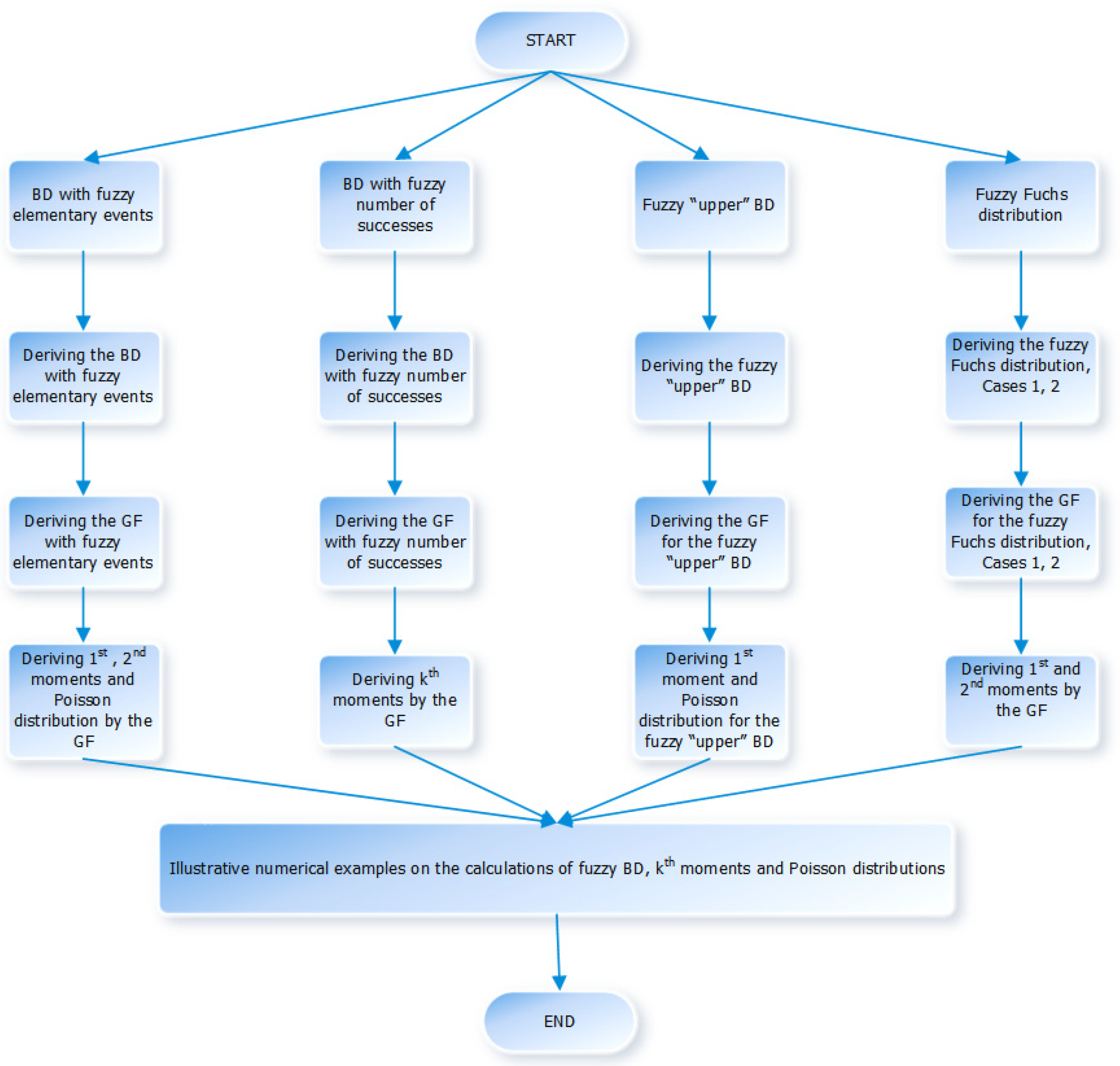
In this work, we present a new approach to the extension of a classical BD under different fuzzy environments. In contrast to the above approaches to the study of fuzzy BDs, a completely new approach is developed in this paper. Section 2 presents the fuzzy extension of the BD, where the Bernoulli fuzzy-random variable is considered instead of the Bernoulli random variable. Success and failure events have both probabilistic distributions and their implementation possibility in the form of compatibility levels. Based on this information, the probabilistic distribution of the corresponding binomial fuzzy-random variable is calculated. The conditions of restrictions on this distribution are obtained. The Poisson distribution is calculated as a limit case of the constructed binomial fuzzy-random experiment. Section 3 considers the fuzzy extension of a BD, where the number of successes, unlike the previous case, is of a fuzzy nature and is represented as a fuzzy subset of the set of possible success numbers. A formula for calculating the probability of the occurrence of binomial dependent fuzzy events is obtained. The formula for calculating the probability of the convolution of binomial dependent fuzzy events is obtained. The invariance principle of exponential distribution is applied, and the corresponding GF is constructed. As a result, a scheme for calculating the mathematical expectation of the number of fuzzy successes is created. Section 4 considers the fuzzy extension of the binomial upper distribution, where the fuzziness is represented in the compatibility levels of the binomial and non-binomial events of the complete failure complex. The GF of the constructed distribution and the first-order moment of the distribution are also calculated. Sufficient conditions for the existence of a corresponding limit distribution and the Poisson distribution are also obtained. Section 5 presents the fuzzy extension of the classical Fuchs distribution, where fuzziness is reflected in the number of increasing failures. The built distribution function and the first and second order moments of the distribution are also calculated. Sufficient conditions for the existence of a corresponding limit distribution and the Poisson distribution are obtained. For better representation of the results, the examples of fuzzy BD are illustrated in each section. Section 6 presents the main results obtained and prospects for future research. A sequential scheme of the key facts and obtained results is presented by Scheme 1.

2. BD by Fuzzy Elementary Events

Consider $P_1$ and $P_0=1-P_1$ as elementary a priori probabilities of success (“1”) and failure (“0”) events, respectively. Let us also consider the membership levels ${\mu }_1$ and ${\mu }_2$ for (1) and (0), respectively. Therefore, we created a fuzzy-random variable of Bernoulli -$\tilde{\mathcal{X}}\sim \left(\begin{array}{ccc}values& 1& 0\\ probabilities& P_1& P_0\\ membership\hspace{0.17em}levels& {\mu }_1& {\mu }_2\end{array}\right)$. Then, the probabilities of the fuzzy events $\tilde{1}$ and $\tilde{0}$ according to [24,25] can be calculated by the formulas:

$$\mathcal{P}(\tilde{1})={\mu }_1{P}_1 \mathrm{and} \mathcal{P}(\tilde{0})={\mu }_2{P}_0$$

(1)

For a sequence of $n$ repetitive ordinary (non-fuzzy) trials in a binomial experiment, we introduce the notations

$$\begin{array}{l}{C}_1\equiv (1,\dots ,1)\hspace{0.17em},\hspace{0.17em}\hspace{0.17em}\hspace{0.17em}\hspace{0.17em}\hspace{0.17em}{C}_2\equiv (1,\dots ,1,0),\dots ,\\ C_{2^n-1}\equiv (0,\dots ,0,1),\hspace{0.17em}\hspace{0.17em}\hspace{0.17em}\hspace{0.17em}{C}_{2^n}\equiv (0,\dots ,0),\end{array}$$

(2)

as there exist $2^n$ possible results by the combination of (1) and (0). For describing the “$n$ repetitive fuzzy elementary experiments”

$${\tilde{C}}_1\equiv (\tilde{1},\dots ,\tilde{1}),\dots ,{\tilde{C}}_{2^n}\equiv (\tilde{0},\dots ,\tilde{0})$$

(3)

We refer to the notion of a fuzzy variable introduced in [24]. Suppose we have a fuzzy Bernoulli variable $\tilde{\mathcal{X}}\equiv (X,U,\tilde{R}(x,u))$, where $X$ is a fuzzy elementary event, $U=\left\{0,1\right\}$ is a universal set, and the restriction $\tilde{R}(x,u)\subset U$ means that

$$\tilde{R}(x,u)\equiv \tilde{R}(\tilde{\mathcal{X}})\equiv \tilde{0}\cup \tilde{1}\equiv \left\{\tilde{0},\tilde{1}\right\},$$

(4)

Consider an ordered set of $n$ such variables $({\tilde{\mathcal{X}}}_1,\dots ,{\tilde{\mathcal{X}}}_n)$ as a fuzzy binomial experiment. According to [24], the universal set of such a compound fuzzy variable is the Cartesian product $U_1\times \dots \times U_n$. Now, suppose that ${\tilde{\mathcal{X}}}_1,\dots ,{\tilde{\mathcal{X}}}_n$ are the same non-interactive variables, i.e.,

$$\tilde{\mathrm{R}}({\tilde{\mathcal{X}}}_1,\dots ,{\tilde{\mathcal{X}}}_n)=\overline{\tilde{R}}({\tilde{\mathcal{X}}}_1)\cap \dots \hspace{0.17em}\cap \overline{\tilde{R}}({\tilde{\mathcal{X}}}_n)$$

(5)

where $\overline{\tilde{R}}({\tilde{\mathcal{X}}}_i)$ is a cylindrical continuation of a marginal constraint $\tilde{R}({\tilde{\mathcal{X}}}_i),\hspace{0.17em}\hspace{0.17em}i=1,\dots ,n$. We refer to the sequence of “$n$ repetitive fuzzy elementary experiments” as a fuzzy point $\tilde{\mathrm{R}}({\tilde{\mathcal{X}}}_1,\dots ,{\tilde{\mathcal{X}}}_n)$. According to (5), we have:

$$\begin{array}{l}{\mu }_{{\tilde{C}}_1}=\min \{{\mu }_1,\dots ,{\mu }_1\},\hspace{0.17em}\hspace{0.17em}{\mu }_{{\tilde{C}}_{2^n}}=\min \{{\mu }_2,\dots ,{\mu }_2\},\hspace{0.17em}\hspace{0.17em}\hspace{0.17em}\\ {\mu }_{{\tilde{C}}_i}=\min \{({\mu }_1\hspace{0.17em}or\hspace{0.17em}{\mu }_2)\wedge \dots \wedge ({\mu }_1\hspace{0.17em}or\hspace{0.17em}{\mu }_2)\}={\mu }_1\wedge \hspace{0.17em}{\mu }_2,\hspace{0.17em}\hspace{0.17em}\hspace{0.17em}i=2,3,\dots ,\hspace{0.17em}{2}^n-1.\end{array}$$

(6)

If we use the formula for calculating a fuzzy event probability, we obtain the following probabilities:

$$\begin{array}{l}\mathcal{P}\left({\tilde{C}}_1\right)\equiv \mathcal{P}(\tilde{1},\dots ,\tilde{1},\tilde{1})={\mu }_{1}P(1,\dots ,1,1)\\ \mathcal{P}\left({\tilde{C}}_2\right)\equiv \mathcal{P}(\tilde{1},\dots ,\tilde{1},\tilde{0})=({\mu }_1\wedge {\mu }_2)P(1,\dots ,1,0),\dots ,\\ \mathcal{P}\left({\tilde{C}}_{2^n-1}\right)\equiv \mathcal{P}(\tilde{0},\dots ,\tilde{0},\tilde{1})=({\mu }_1\wedge {\mu }_2)P(0,\dots ,0,1)\\ \mathcal{P}\left({\tilde{C}}_{2^n}\right)\equiv \mathcal{P}(\tilde{0},\dots ,\tilde{0},\tilde{0})={\mu }_{2}P(0,\dots ,0,0).\end{array}$$

(7)

As is well known, the projection of a relation on a given set of variables is a marginal sub-relation of that relation which applies only on these variables. It is considered on the Cartesian product of the universes of these variables. If we sum the distribution (7) by the projection of relation (5)

$$\underset{U_{i_1}\times \dots \times U_{i_{n-1}}}{{\displaystyle \mathrm{Proj}}}\hspace{0.17em}\langle \tilde{\mathrm{R}}({\tilde{\mathcal{X}}}_1,\dots ,{\tilde{\mathcal{X}}}_n)\rangle \hspace{0.17em}\hspace{0.17em}={\tilde{R}}_q\left({\tilde{\mathcal{X}}}_{i_1},\dots , {\tilde{\mathcal{X}}}_{i_{n-1}}\right),\hspace{0.17em}\hspace{0.17em}\hspace{0.17em}\hspace{0.17em}\hspace{0.17em}\hspace{0.17em}\hspace{0.17em}q\equiv ( i_1,\dots ,i_{n-1}),$$

(8)

we receive only normed fuzzy probabilities of $\tilde{1}$ and $\tilde{0}$

$$\mathcal{P}(\tilde{1})=\frac{{\mu }_1{P}_1}{{\sum }_{i=1}^{2^n}\mathcal{P}\left({\tilde{C}}_i\right)},$$

(9)

$$\mathcal{P}(\tilde{0})=1-\mathcal{P}(\tilde{1})=\frac{{\mu }_1{P}_0+({\mu }_2-{\mu }_1)P(0,\dots ,0)}{{\sum }_{i=1}^{2^n}\mathcal{P}\left({\tilde{C}}_i\right)}.$$

After substituting (7) and (9) in the BD formula, we receive:

$$\begin{array}{l}\mathcal{P}({\tilde{C}}_{(k)})=\frac{P_1^k}{{[1+(\frac{{\mu }_2}{{\mu }_1}-1)P(0,\dots ,0)]}^{n-1}}{[1+(\frac{{\mu }_2}{{\mu }_1}-1)P(0,\dots ,0)-P_1]}^{n-k},\\ k=1,\dots ,n.\end{array}$$

(10)

where common notation ${\tilde{C}}_{\left(k\right)}$ is introduced for those ${\tilde{C}}_i$ to which the same number $k$ of successes correspond, since the probabilities of such ${\tilde{C}}_i$ are equal. Note that

$$\sum _{i=1}^{2^n}\mathcal{P}({\tilde{C}}_i)={\mu }_1+({\mu }_2-{\mu }_1)P(0,\dots ,0),$$

(11)

It is clear from (9) and (10) that if ${\mu }_1={\mu }_2$, then the conditions for the independence of fuzzy events degenerate to the corresponding conditions for ordinary events.

The constraint (7) for probabilities $\mathcal{P}({\tilde{C}}_{(k)})$ leads to the relationship

$$\frac{{\mu }_2}{{\mu }_1}={\left[1+\frac{1-P_1\cdot \sqrt[n-1]{\frac{P_1}{P\left(1, \dots ,1\right)}}}{P\left(1, \dots ,1\right){\left(\sqrt[n-1]{\frac{P_1}{P\left(1, \dots ,1\right)}}-1\right)}^n}\right]}^{-1}.$$

(12)

By putting Formula (12) into (11) and assuming that ${\mu }_2\ge {\mu }_1$ and $\mathcal{P}\left({\tilde{C}}_i\right)\ge 0$, we get a system of conditions

$$\mathcal{P}\left({\tilde{C}}_{(k)}\right)=P(1,\dots ,1){[\sqrt[n-1]{\frac{P_1}{P(1,\dots ,1)}}-1]}^{n-k},k=1,\dots ,n;$$

(13)

$$0\le \frac{P_1\cdot \sqrt[n-1]{\frac{P_1}{P\left(1, \dots ,1\right)}}-1}{P\left(1, \dots ,1\right){\left[\sqrt[n-1]{\frac{P_1}{P\left(1, \dots ,1\right)}}-1\right]}^n}<1; \frac{{\mu }_2}{{\mu }_1}=1+\frac{-1+P_1\cdot \sqrt[n-1]{\frac{P_1}{P\left(1, \dots ,1\right)}}}{P\left(0, \dots ,0\right)}.$$

(14)

The probabilities of considering fuzzy events, normalized in $\tilde{\mathrm{R}}({\tilde{\mathcal{X}}}_1,\dots ,{\tilde{\mathcal{X}}}_n)={\displaystyle \underset{i=1}{\overset{2^n}{\cup }}{\tilde{C}}_i}$, are calculated by the formula

$${\mathcal{P}}^{\prime }({\tilde{C}}_i)=\frac{\mathcal{P}({\tilde{C}}_i)}{{\sum }_{j=1}^{2^n}\mathcal{P}({\tilde{C}}_j)},i=1,\dots ,2^n.$$

(15)

In deriving the BD with fuzzy elementary events, we will proceed from the notion of the independence of fuzzy events [23], which is not equivalent to the ordinary independence. This leads to the certain conditions of independence, which we discuss below. For the purpose of clarity, let ${\mu }_1\le {\mu }_2$; then, we obtain the fuzzy binomial distribution:

$${\mathcal{P}}^{\prime }\left({\tilde{C}}_1\right)={[{\mathcal{P}}^{\prime }(\tilde{1})]}^n,\dots ,{\mathcal{P}}^{\prime }\left({\tilde{C}}_{2^n}\right)={[{\mathcal{P}}^{\prime }(\tilde{0})]}^n$$

Thus, conditions (13)–(15) are equivalent to the existence of the $n$-ar fuzzy-random variable, which is a sequence of $n$ repetitive, fuzzy, non-interacting, and independent elementary events whose distribution is described by the BD with fuzzy elementary events

$$\begin{array}{l}{\mathcal{P}}^{\prime }\left({\tilde{\mathcal{B}}}_n^k\right)=C_n^k{[{\mathcal{P}}^{\prime }(\tilde{1})]}^k{[{\mathcal{P}}^{\prime }(\tilde{0})]}^{n-k}=C_n^k\frac{{\mu }_1^k{P}_1^k{[{\mu }_1{P}_0+({\mu }_2-{\mu }_1)P(0\dots ,0)]}^{n-k}}{{[{\mu }_1+({\mu }_2-{\mu }_1)P(0,\dots 0)]}^n}=\\ C_n^k\frac{P_1^k{[P_0+(\frac{{\mu }_2}{{\mu }_1}-1)P(0,\dots ,0)]}^{n-k}}{{[1+(\frac{{\mu }_2}{{\mu }_1}-1_1)P(0,\dots 0)]}^n},\end{array}$$

(16)

where

$${\widetilde{ℬ}}_n^k={\displaystyle \underset{\forall j \mathrm{with} k \mathrm{successes}}{\cup }{\tilde{C}}_j}.$$

If ${\mu }_2<{\mu }_1$, for the calculation of ${\mathcal{P}}^{\prime }\left({\tilde{\mathcal{B}}}_n^k\right)$, it is necessary to make the following changes in the ending part of Equation (16). Instead of $\frac{{\mu }_2}{{\mu }_1}$, we write $\frac{{\mu }_1}{{\mu }_2}$, and instead of $P\left(0,\dots ,0\right)$, we write $P\left(1,\dots ,1\right)$:

$$\frac{{\mu }_2}{{\mu }_1}\leftarrow \frac{{\mu }_1}{{\mu }_2}\hspace{0.17em},\hspace{0.17em}\hspace{0.17em}\hspace{0.17em}\hspace{0.17em}\hspace{0.17em} P\left(0,\dots ,0\right)\leftarrow P\left(1,\dots ,1\right).$$

To be more precise, we receive

$$\begin{array}{l}{\mathcal{P}}^{\prime }\left({\tilde{\mathcal{B}}}_n^k\right)=C_n^k\frac{{[{\mu }_2{P}_1+({\mu }_1-{\mu }_2)P(1,\dots ,1)]}^k{\mu }_2^{n-k}{P}_0^{n-k}}{{[{\mu }_2+({\mu }_1-{\mu }_2)P(1,\dots ,1)]}^n},\\ C_n^k\frac{P_0^{n-k}{[P_1+(\frac{{\mu }_1}{{\mu }_2}-1)P(1,\dots ,1)]}^{n-k}}{{[1+(\frac{{\mu }_1}{{\mu }_2}-1)P(1,\dots ,1)]}^n}.\end{array}$$

(17)

Note that in both cases, if ${\mu }_2={\mu }_1$, then (16) and (17) transform to the usual BD.

From Formulas (16) and (17), we see that ${\mathcal{P}}^{\prime }\left({\tilde{\mathcal{B}}}_n^k\right)$ depends on the ratio $\frac{{\mu }_2}{{\mu }_1}$ if ${\mu }_2>{\mu }_1$, and on the ratio $\frac{{\mu }_1}{{\mu }_2}$ if ${\mu }_2<{\mu }_1$, while the condition of independence and non-interaction (14) allows us to express the normalized probability ${\mathcal{P}}^{\prime }\left({\tilde{\mathcal{B}}}_n^k\right)$ with the probabilities of the corresponding non-fuzzy events. Indeed, it is not difficult to show that

$${\mathcal{P}}^{\prime }(\tilde{1})=\{\begin{array}{ll}\sqrt[n-1]{P_1(\stackrel{n-1}{\overbrace{1,\dots ,1)}}},& {\mu }_1<{\mu }_2\\ \sqrt[n-1]{P_0(\stackrel{n-1}{\overbrace{1,\dots ,1)}}},& {\mu }_1>{\mu }_2\end{array}, {\mathcal{P}}^{\prime }(\tilde{0})=\{\begin{array}{ll}\sqrt[n-1]{P_1(\stackrel{n-1}{\overbrace{0,\dots ,0)}}},& {\mu }_1<{\mu }_2\\ \sqrt[n-1]{P_0(\stackrel{n-1}{\overbrace{0,\dots ,0)}}},& {\mu }_1>{\mu }_2\end{array}$$

(18)

If we enter the values from Formula (18) to Formulas (16) and (17), we get

$${\mathcal{P}}^{\prime }\left({\tilde{\mathcal{B}}}_n^k\right)=\{\begin{array}{l}{C}_n^k[P_1(\stackrel{n-1}{\overbrace{1,\dots ,1)}}{]}^{\frac{k}{n-1}}[P_1(\stackrel{n-1}{\overbrace{0,\dots ,0)}}{]}^{\frac{n-k}{n-1}},{\mu }_1<{\mu }_2,\\ C_n^k[P_0(\stackrel{n-1}{\overbrace{1,\dots ,1)}}{]}^{\frac{k}{n-1}}[P_0(\stackrel{n-1}{\overbrace{0,\dots ,0)}}{]}^{\frac{n-k}{n-1}},{\mu }_1>{\mu }_2.\end{array}$$

(19)

Using the notion of a discrete distribution moment generating function, we analytically obtain the formula of the GF of the BD with fuzzy elementary events (two cases are considered as presented above).

$$G_{{\mathcal{P}}^{\prime }\left({\hat{\mathfrak{B}}}_n^k\right)}(y)=\{\begin{array}{l}\frac{{[{\mu }_1{P}_0+{\mu }_1{P}_{1}y+({\mu }_2-{\mu }_1)P(0,\dots ,0)]}^n}{{[{\mu }_1+({\mu }_2-{\mu }_1)P(0,\dots ,0)]}^n},{\mu }_1<{\mu }_2,\\ \frac{{[{\mu }_2{P}_{1}y+({\mu }_1-{\mu }_2)P(1,\dots ,1)y+{\mu }_2{P}_0]}^n}{{[{\mu }_2+({\mu }_1-{\mu }_2)P(1,\dots ,1)]}^n},{\mu }_1>{\mu }_2.\end{array}$$

(20)

As is well known, distribution moments are easily calculated from the generating function. Without presenting a long process of calculation, we give the analytical form of the first and second order moments of the BD with fuzzy elementary events

$$\overline{k}=\{\begin{array}{c}\frac{n{\mu }_1{P}_1}{{\mu }_1+\left({\mu }_2-{\mu }_1\right)P\left(0, \dots ,0\right)}\\ \frac{n[{\mu }_2{P}_1+\left({\mu }_1-{\mu }_2\right)P\left(1, \dots ,1\right)]}{{\mu }_2+\left({\mu }_1-{\mu }_2\right)P\left(1, \dots ,1\right)}\end{array}\hspace{0.17em}\begin{array}{c}, {\mu }_1<{\mu }_2,\\ \\ , {\mu }_1>{\mu }_2.\end{array}=\{\begin{array}{c}\frac{n{P}_1}{1+\left(\frac{{\mu }_2}{{\mu }_1}-1\right)P\left(0, \dots ,0\right)}\\ \frac{n[P_1+\left(\frac{{\mu }_1}{{\mu }_2}-1\right)P\left(1, \dots ,1\right)]}{1+\left(\frac{{\mu }_1}{{\mu }_2}-1\right)P\left(1, \dots ,1\right)}\end{array}\hspace{0.17em}\begin{array}{c}, {\mu }_1<{\mu }_2,\\ \\ , {\mu }_1>{\mu }_2.\end{array}$$

(21)

$$\begin{gathered} {\overline{k}}^2=\overline{k}(1+\frac{n-1}{n}\overline{k})=\{\begin{array}{c}\frac{n{\mu }_1{P}_1}{{\mu }_1+\left({\mu }_2-{\mu }_1\right)P\left(0, \dots ,0\right)}\left[1+\frac{\left(n-1\right){\mu }_1{P}_1}{{\mu }_1+\left({\mu }_2-{\mu }_1\right)P\left(0, \dots ,0\right)}\right]\\ \frac{n[{\mu }_2{P}_1+\left({\mu }_1-{\mu }_2\right)P\left(1, \dots ,1\right)]}{{\mu }_2+\left({\mu }_1-{\mu }_2\right)P\left(1, \dots ,1\right)}\left[1+\frac{\left(n-1\right)[{\mu }_2{P}_1+\left({\mu }_1-{\mu }_2\right)P\left(1, \dots ,1\right)]}{{\mu }_2+\left({\mu }_1-{\mu }_2\right)P\left(1, \dots ,1\right)}\right]\end{array}\hspace{0.17em}\hspace{0.17em}\begin{array}{c}, {\mu }_1<{\mu }_2,\\ \\ , {\mu }_1>{\mu }_2.\end{array} \\ =\{\begin{array}{c}\frac{n{P}_1}{1+\left(\frac{{\mu }_2}{{\mu }_1}-1\right)P\left(0, \dots ,0\right)}\left[1+\frac{\left(n-1\right)P_1}{1+\left(\frac{{\mu }_2}{{\mu }_1}-1\right)P\left(0, \dots ,0\right)}\right]\\ \frac{n[P_1+\left(\frac{{\mu }_1}{{\mu }_2}-1\right)P\left(1, \dots ,1\right)]}{1+\left(\frac{{\mu }_1}{{\mu }_2}-1\right)P\left(1, \dots ,1\right)}\left[1+\frac{(n-1)P_1+\left(\frac{{\mu }_1}{{\mu }_2}-1\right)P\left(1, \dots ,1\right)]}{1+\left(\frac{{\mu }_1}{{\mu }_2}-1\right)P\left(1, \dots ,1\right)}\right]\end{array}\hspace{0.17em}\hspace{0.17em}\begin{array}{c}, {\mu }_1<{\mu }_2,\\ \\ , {\mu }_1>{\mu }_2.\end{array} \end{gathered}$$

(22)

Expressions (16), (17), and (21) allow us to prove the existence of Poisson limits for BD with fuzzy elementary events. It is not difficult to calculate the limits below if we use a well-known numerical sequence limit calculation technique. There are some possible cases:

(1). $\overline{k}=const.$ In this case, we obviously have

$$\underset{\begin{array}{c}n\to \infty \\ \overline{\mathrm{k}}=const\end{array}}{\lim }{\mathcal{P}}^{\prime }\left({\tilde{\mathcal{B}}}_n^k\right)=e^{-\overline{k}}\frac{{\overline{k}}^k}{k!},k=0,1,\dots$$

(23)

(2). ${\mu }_{{}_1}$ and ${\mu }_2$ are fixed and $n{P}_1=const$. It is easy to show that:

$$\underset{\begin{array}{l}n\to \infty \\ n{P}_1=\lambda =\mathit{const}\\ P_1\to 0\end{array}}{\lim }{\mathcal{P}}^{\prime }\left({\tilde{\mathcal{B}}}_n^k\right)=\{\begin{array}{ll}{e}^{-c^{\prime }}\frac{{\left(c^{\prime }\right)}^k}{k!},& c^{\prime }=\frac{\lambda }{1+(\frac{{\mu }_2}{{\mu }_1}-1)[P(\overbrace{0,\dots ,0})]},{\mu }_1<{\mu }_2,\\ e^{-c^{″}}\frac{{\left(c^{″}\right)}^k}{k!}& c^{″}=\lambda +(\frac{{\mu }_1}{{\mu }_2}-1)[P(\stackrel{n}{\overbrace{1,\dots ,1}})],{\mu }_1>{\mu }_2.\end{array}$$

(24)

Example 1.

Let the fuzzy Bernoulli distribution be given $\tilde{\mathcal{X}}\sim \left(\begin{array}{ccc}values& 1& 0\\ probabilities& 0.3& 0.7\\ membership\hspace{0.17em}levels& 0.5& 0.6\end{array}\right)$. Based on Formula (19), construct fuzzy BD for the $n=5$. Use Formulas (21) and (22) and calculate the moments of the first and second order $\overline{k}$ and ${\overline{k}}^2$. Calculate the standard deviation of distribution $SD=\sqrt{{\overline{k}}^2-{(\overline{k})}^2}$. Using the Poisson distribution Formula (24), calculate the distribution values for $k=0,1,\dots ,7$ when $n{P}_1\simeq const=6$.

Solution of Example 1. It is clear that for the calculations $P_1=0.3$ and $P_0=0.7$, ${\mu }_1=0.5$ and ${\mu }_2=0.6$, $n=5$, $k=0,1,2,3,4,5$. In our case, ${\mu }_1<{\mu }_2$. Let us assume that $P_1(\stackrel{n-1}{\overbrace{0,\dots ,0)}}$ = $P_1(\stackrel{4}{\overbrace{0,\dots ,0)}}={(0.7)}^4$ and $P_1(\stackrel{n-1}{\overbrace{1,\dots ,1)}}$=$P_1(\stackrel{4}{\overbrace{1,\dots ,1)}}={(0.3)}^4$. We receive (

Table 1. Conditional fuzzy binomial probability distribution.

$\mathit{k}$	0	1	2	3	4	5
${\mathcal{P}}^{\prime }\left({\tilde{\mathcal{B}}}_n^k\right)$	0.1681	0.3601	0.3087	0.1323	0.0283	0.0024

).

Using Formulas (21) and (22), we receive $\overline{k}$ = 1.4512, ${\overline{k}}^2$ = 3.1360, and $SD=\sqrt{{\overline{k}}^2-{(\overline{k})}^2}$ = 1.0149. For the Poisson distribution, if $n{P}_1\simeq const=6$, then, for $k=0,1,2,3,4,5$, we receive (

Table 2. Fragment of Poisson distribution.

$\mathit{k}$	0	1	2	3	4	5	6	7
$\underset{\begin{array}{c}n\to \infty \\ n{P}_1=\mathit{const}\end{array}}{\lim }{\mathcal{P}}^{\prime }\left({\tilde{\mathcal{B}}}_n^k\right)$	0.0029	0.0170	0.0497	0.0967	0.1411	0.1647	0.1603	0.1336

).

3. BDs with a Fuzzy Number of Successes

Consider a set ${\mathcal{A}}_n\equiv \left\{0, 1, \dots , n\right\}.$ Let $\tilde{k},\hspace{0.17em}\hspace{0.17em}\tilde{k}\subset {\mathcal{A}}_n$ be the fuzzy subset in ${\mathcal{A}}_n$, $\tilde{k}=“approximately\hspace{0.17em}\hspace{0.17em}k\hspace{0.17em}\hspace{0.17em}number”$ with some membership function ${\mu }_{\tilde{k}}:\hspace{0.17em}{\mathcal{A}}_n\to [0,1]$ and $\tilde{k}={\displaystyle \underset{l=0}{\overset{n}{\cup }}\left[{\mu }_{\tilde{k}}\left(l\right)/l\right]}$ [23,24].

If ${\mathcal{A}}_n$ is a set of numbers of possible successes in $n$ trials of the binomial scheme, then it is well known that to each element of ${\mathcal{A}}_n$ corresponds the probability $P({ℬ}_{n;p}^k)=C_n^k{p}^k{q}^{n-k}$. Therefore, according to [24,25], for the BD with the fuzzy success number, we obtain the formula

$$\mathcal{P}\left({\mathcal{B}}_{n;p}^{\tilde{k}}\right)={\sum }_{l=0}^n{\mu }_{\tilde{k}}(l)P\left({\mathcal{B}}_{n;p}^l\right)$$

(25)

Here, $\mathcal{P}\left({\tilde{\mathcal{B}}}_{n;p}^k\right)$ is the probability measure of a fuzzy event ${ℬ}_{n;p}^{\tilde{k}}$ or the fuzzy subset $\tilde{k}$.

Note that in this scheme under consideration, the fuzzy events ${ℬ}_{n;p}^{\tilde{k}}$ are not mutually exclusive events. Therefore, according to the additivity property of a probability measure of a fuzzy event [24,25], we have

$$\begin{array}{l}\mathcal{P}\left(\underset{k=0}{\overset{n}{\cup }}{\mathcal{B}}_{n;p}^{\tilde{k}}\right)={\sum }_{k=0}^n\mathcal{P}\left({\mathcal{B}}_{n;p}^{\tilde{k}}\right)-{\displaystyle \sum _{k,k^{\prime }}}\mathcal{P}({\mathcal{B}}_{n;p}^{\tilde{k}}\cap {\mathcal{B}}_{n;p}^{\widetilde{k^{\prime }}})+{\displaystyle \sum _{k,k^{\prime },k^{″}}}\mathcal{P}({\mathcal{B}}_{n;p}^{\tilde{k}}\cap {\mathcal{B}}_{n;p}^{\widetilde{k^{\prime }}}\cap {\mathcal{B}}_{n;p}^{\widetilde{k^{″}}})+\dots \\ +(-1{)}^n\mathcal{P}({\mathcal{B}}_{n;p}^{\tilde{o}}\cap \dots \cap {\mathcal{B}}_{n;p}^{\tilde{n}}).\end{array}$$

(26)

Let $0<p_i<1,\hspace{0.17em}\hspace{0.17em}i=1,2$ be two numbers. An important feature of the distribution (25) is that the law of composition is satisfied

$$\mathcal{P}\left({\mathcal{B}}_{n;p_1{p}_2}^{\tilde{k}}\right)={\sum }_{m=0}^{n}P\left({\mathcal{B}}_{n;p_1}^m\right)\mathcal{P}\left({\mathcal{B}}_{m,p_2}^{\tilde{k}}\right)$$

(27)

which is easily verified by the simple calculations

$$\mathcal{P}\left({\mathcal{B}}_{n;p_1{p}_2}^{\tilde{k}}\right)={\sum }_{l=0}^n{\mu }_{\tilde{k}}(l)P\left({\mathcal{B}}_{n;p_1{p}_2}^l\right)={\sum }_{l=0}^n{\mu }_{\tilde{k}}(l)C_n^k{\left(p_1{p}_2\right)}^l{(1-p_1{p}_2)}^{n-l}$$

and

$$\begin{array}{l}{\sum }_{m=0}^{n}P\left({\mathcal{B}}_{n;p_1}^m\right)\mathcal{P}\left({\mathcal{B}}_{m,p_2}^{\tilde{k}}\right)={\sum }_{m=0}^{n}P\left({\mathcal{B}}_{n;p_1}^m\right){\sum }_{l=0}^n{\mu }_{\tilde{k}}(l)P\left({\mathcal{B}}_{n;p_2}^l\right)=\\ {\sum }_{l=0}^n{\mu }_{\tilde{k}}(l){\sum }_{m=0}^n{C}_n^m{C}_m^l{p}_1^m{(1-p_1)}^{n-m}{p}_2^l{(1-p_2)}^{m-l}={\sum }_{l=0}^n{\mu }_{\tilde{k}}(l)\frac{n!}{l!(n-l)!}{\left(p_1{p}_2\right)}^l{(1-p_1{p}_2)}^{n-l}\\ \times {\sum }_{m=0}^n\frac{(n-l)!}{(n-m)!(m-l)!}\frac{p_1^{m-l}{(1-p_1)}^{n-m}{(1-p_2)}^{m-l}}{{(1-p_1{p}_2)}^{n-l}}={\sum }_{l=0}^n{\mu }_{\tilde{k}}(l)\frac{n!}{l!(n-l)!}{p}_1{p}_2^l{(1-p_1{p}_2)}^{n-l}\\ \times {\sum }_{j=0}^{n-l}\frac{(n-l)!}{j!(n-l-j)!}\frac{p_1^j{(1-p_1)}^{n-l-j}{(1-p_2)}^j}{{(1-p_1{p}_2)}^{n-l}}={\sum }_{l=0}^n{\mu }_{\tilde{k}}(l)P\left({\mathcal{B}}_{n;p_1{p}_2}^l\right).\end{array}$$

Based on the property of the invariability of the exponential distribution, let us extend the fuzzy subset $\tilde{k}$ from the set ${\mathcal{A}}_n$ to the non-negative integer numbers set $N\cup \{0\}$. In this case, the extended membership function ${\mu }_{\tilde{k}}\left(l\right),\hspace{0.17em}\hspace{0.17em}\hspace{0.17em}l\in N\cup \left\{0\right\}$ will be a mapping of a set of natural numbers $\mathbb{N}$ into $\left[0,1\right]$. Consider the expression of the moments’ generating function of fuzzy BD.

Consider the expression of the moments’ GF of the fuzzy BD

$$G(\tilde{k})={\sum }_{n=0}^{\infty }\mathcal{P}\left({\mathcal{B}}_{n;p}^{\tilde{k}}\right)f_n(u),$$

(28)

where $f_n\left(u\right)=\left(1-u\right)u^n, 0<u<1$.

If we denote $v=\frac{pu}{1-u+pu}$ and $g_l\left(v\right)=\left(1-v\right)v^l$, then

$$G(\tilde{k})={{\displaystyle \sum }}_{l=0}^{\infty }{\mu }_{\tilde{k}}\left(l\right)g_l\left(v\right).$$

(29)

Indeed,

$$\begin{array}{l}G(\tilde{k})={\sum }_{n=0}^{\infty }{f}_n(u)\mathcal{P}\left({\mathcal{B}}_{n;p}^{\tilde{k}}\right)={\sum }_{n=0}^{\infty }{f}_n(u){\sum }_{l=0}^n{\mu }_{\tilde{k}}(l)P\left({\mathcal{B}}_{n;p}^l\right)=f_0(u){\sum }_{l=0}^0{\mu }_{\tilde{k}}(l)P\left({\mathcal{B}}_{0;p}^l\right)\\ +f_1(u){\sum }_{l=0}^1{\mu }_{\tilde{k}}(l)P\left({\mathcal{B}}_{1;p}^l\right)+f_2(u){\sum }_{l=0}^2{\mu }_{\tilde{k}}(l)P\left({\mathcal{B}}_{2;p}^l\right)+\dots \\ ={\mu }_{\tilde{k}}(0)[f_0(u)P\left({\mathcal{B}}_{0;p}^0\right)+f_1(u)P\left({\mathcal{B}}_{1;p}^0\right)+f_2(u)P\left({\mathcal{B}}_{2;p}^0\right)+\dots ]+\\ {\mu }_{\tilde{k}}(1)[f_1(u)P\left({\mathcal{B}}_{1;p}^1\right)+f_2(u)P\left({\mathcal{B}}_{2;p}^1\right)+\dots ]\\ +{\mu }_{\tilde{k}}(2)[f_2(u)P\left({\mathcal{B}}_{2;p}^2\right)+f_3(u)P\left({\mathcal{B}}_{3;p}^2\right)+\dots ]+\dots \end{array}$$

Given that for $r<s$ $P\left({ℬ}_{r;p}^s\right)=0$, then

$$\begin{array}{l}G\left(\tilde{k}\right)={{\displaystyle \sum }}_{n=0}^{\infty }{\mu }_{\tilde{k}}\left(n\right){{\displaystyle \sum }}_{l=0}^{\infty }{f}_l\left(u\right)P\left({ℬ}_{l;p}^n\right)\\ ={{\displaystyle \sum }}_{n=0}^{\infty }{\mu }_{\tilde{k}}\left(n\right){{\displaystyle \sum }}_{l=0}^{\infty }\begin{array}{c}\frac{l!}{n!\left(n-l\right)!}{p}^n{\left(1-p\right)}^{l-n}\left(1-u\right)u^l\end{array}\\ ={{\displaystyle \sum }}_{n=0}^{\infty }{\mu }_{\tilde{k}}\left(n\right)\left(1-u\right){\left(pu\right)}^n{{\displaystyle \sum }}_{l=0}^{\infty }\frac{l!}{n!\left(n-l\right)!}{\left[\left(1-p\right)u\right]}^{l-n}=\\ {{\displaystyle \sum }}_{n=0}^{\infty }{\mu }_{\tilde{k}}\left(n\right)\left(1-u\right){\left(pu\right)}^n{{\displaystyle \sum }}_{j=0}^{\infty }\frac{\left(n+j\right)!}{n!j!}\left[(1-p\right)u{]}^j\hspace{0.17em}\hspace{0.17em}\hspace{0.17em}.\end{array}$$

The last sum is a decomposition of the function ${\left[1-\left(1-p\right)u\right]}^{-n+1}$ into series by degrees of $(1-p)u$. Considering the connection between $u$ and $v$, we finally obtain the expression of (29)

$$G\left(\tilde{k}\right)={{\displaystyle \sum }}_{n=0}^{\infty }{\mu }_{\tilde{k}}\left(l\right)\frac{1-u}{1-\left(1-p\right)u}{\left[\frac{pu}{1-\left(1-p\right)u}\right]}^n.$$

To determine the mean value of a success fuzzy number “with probability measure $\mathcal{P}$”, let us do the following. Consider a set of ordinary (nonfuzzy) events $\mathcal{A}\subset {\mathcal{A}}_n$. Define the function of a set $E(.)$ in such a way that, for any subset $\mathcal{A}$, this function corresponds to the conditional mean, i.e., if $\mathcal{A}\subset {\mathcal{A}}_n$, then $E(\mathcal{A})={\overline{k}}_{\mathcal{A}}$. According to the principle of generalization [23], the domain of definition $E(.)$ can be extended to fuzzy subsets as well. Suppose we have a fuzzy subset $\tilde{k}$ of ${\mathcal{A}}_n$, and $\tilde{k}$ is represented as

$$\tilde{k}={\displaystyle \underset{\alpha }{\cup }{\mathcal{A}}_{\alpha }}, \alpha \in \left[0,1\right],$$

(30)

where ${\mathcal{A}}_{\alpha }$ denotes a cut set of level $\alpha$. Then,

$$E(\tilde{k})={\displaystyle \underset{\alpha }{\cup }E({\mathcal{A}}_{\alpha })}={\displaystyle \underset{\alpha }{\cup }{\overline{k}}_{{\mathcal{A}}_{\alpha }}}.$$

(31)

Here, $E(\tilde{k})$ is a fuzzy subset on the set of all conditional mean values $ℰ$. Relationships (30) and (31) define the calculation rule for the values of the characteristic functions of fuzzy subsets on the set of all conditional means $\mu \left({\overline{k}}_{\mathcal{A}}\right)$ corresponding to ordinary subsets ${\mathcal{A}}_n$ over ${\mu }_{\tilde{k}}\left(l\right)$.

Define the mean value of the fuzzy success number as a convex combination [23] of the fuzzy subsets $E(\tilde{k})$ with the following weights: $W_n(\tilde{k})=\frac{\mathcal{P}\left({\mathcal{B}}_{n;p}^{\tilde{k}}\right)}{\sum _l\mathcal{P}\left({\mathcal{B}}_{n;p}^{\tilde{l}}\right)}$. We define a fuzzy subset with the following membership function

$${\mu }_{{\tilde{k}}_p}\left(\overline{l_{\mathcal{A}}}\right)=\sum _{\tilde{k}\in {\mathcal{A}}_n}{W}_n(\tilde{k}){\mu }_{\mathrm{E}(\tilde{k})}\left({\overline{l}}_{\mathcal{A}}\right),{\overline{l}}_{\mathcal{A}}\in \mathcal{E}$$

(32)

Note that when ${\mu }_{\tilde{u}}\left(l\right)\to {\delta }_{l_{ }k},\hspace{0.17em}\hspace{0.17em}{\delta }_{l_{ }k}=\{\begin{array}{l}1,\hspace{0.17em}\hspace{0.17em}if\hspace{0.17em}\hspace{0.17em}l=k,\\ 0,\hspace{0.17em}\hspace{0.17em}if\hspace{0.17em}l\ne k\end{array}$, that is, when moving $\tilde{k}$ to the ordinary set $\left\{k\right\},$ “the average by the measure $\mathcal{P}$” tends to the mathematical expectation of the number of successes of the BD, ${\tilde{k}}_{\mathcal{P}}\to np$. The method given here can be used for the calculation of any order fuzzy moments ${\tilde{k}}_{\mathcal{P}}^r$, but when calculating high-order moments, it is necessary to use a certain rule for multiplying fuzzy numbers. Most importantly, we present a rule that is derived from the principle of generalization [23].

The discussion of the Poisson and Normal approximations for (25) is reduced to the substitution of the corresponding approximate values of $P\left({ℬ}_{n;p}^l\right)$ in this formula.

Example 2.

Let the Bernoulli distribution be given $\mathcal{X}\sim \left(\begin{array}{l}values\hspace{0.17em}\hspace{0.17em}\hspace{0.17em}\hspace{0.17em}\hspace{0.17em}\hspace{0.17em}\hspace{0.17em}\hspace{0.17em}\hspace{0.17em}\hspace{0.17em}\hspace{0.17em}1\hspace{0.17em}\hspace{0.17em}\hspace{0.17em}\hspace{0.17em}\hspace{0.17em}\hspace{0.17em}\hspace{0.17em}\hspace{0.17em}\hspace{0.17em}0\\ propbabilities\hspace{0.17em}\hspace{0.17em}\hspace{0.17em}\hspace{0.17em}0.3\hspace{0.17em}\hspace{0.17em}\hspace{0.17em}\hspace{0.17em}\hspace{0.17em}0.7\end{array}\right)$ and let a binomial experiment be created based on this Bernoulli experiment for $n=6$. Let be given the following fuzzy subsets “approximately $k$ successes” ($k=0,\dots ,6$) (

Table 3. Fuzzy subsets “approximately $k$ successes” ($k=0,1,2,3,4,5,6$ ).

$\tilde{\mathit{k}}$$\backslash \mathit{k}$	0	1	2	3	4	5	6
$\tilde{0}$	1.0	0.8	0.6	0.5	0.3	0.2	0.1
$\tilde{1}$	0.9	1.0	0.8	0.6	0.5	0.3	0.1
$\tilde{2}$	0.7	0.8	1.0	0.9	0.6	0.4	0.2
$\tilde{3}$	0.4	0.6	0.8	1.0	0.9	0.7	0.5
$\tilde{4}$	0.2	0.3	0.5	0.8	1.0	0.8	0.6
$\tilde{5}$	0.1	0.3	0.5	0.7	0.9	1.0	0.8
$\tilde{6}$	0.1	0.2	0.3	0.5	0.7	0.9	1.0

).

Use the results of this Section to calculate the numerical values of BD with fuzzy success numbers.

Solution of Example 2. Note that $p=0.3$. Using expression (25) and the data of Table 3, we calculate the BD values presented in

Table 4. Numerical values of BD with fuzzy success numbers—$\mathcal{P}\left({\mathcal{B}}_{n;p}^{\tilde{k}}\right)$.

$\tilde{\mathit{k}}$	$\tilde{0}$	$\tilde{1}$	$\tilde{2}$	$\tilde{3}$	$\tilde{4}$	$\tilde{5}$	$\tilde{6}$
$\mathcal{P}\left({\mathcal{B}}_{n;p}^{\tilde{k}}\right)$	0.6667	0.8118	0.8552	0.7342	0.4927	0.4586	0.3137

.

4. Fuzzy “Upper” BD

As is well known, the discussion on the (non-fuzzy) “upper” BD is based on a model of the superposition of two processes: the binomial process ${ℬ}_{n;p}^k$ and the process of “increasing the total number of failures” ${ℬ}_0$-denoted by ${ℬ}_0\circ {ℬ}_{n;p}^k$, characterized by a priori probability $P({ℬ}_0)=1-\gamma$ [26], where $p$ is the elementary event probability of (“1”). Let ${\mu }_0$ and ${\mu }_0^{\prime }$ be the values of the membership function that correspond to the complex events $\stackrel{n}{\overbrace{(0,\dots ,0)}}$ at attempting to distinguish the binomial and non-binomial origin events. Then, as it is easy to verify, the probability of $k$ successes in $n$ trials of the binomial “upper” fuzzy experiment—denoted by ${\widetilde{ℬ}}_0\circ {ℬ}_{n;p}^k$ will have the form

$$\begin{array}{l}\mathcal{P}({\tilde{\mathcal{B}}}_0\circ {\mathcal{B}}_{n;p}^k)=\frac{1}{Z}\{\begin{array}{c}{\mu }_{0}P\left({\mathcal{B}}_0\right)+{\mu }_0^{\prime }P\left({\overline{\mathcal{B}}}_0\right)P\left({\mathcal{B}}_{n;p}^0\right),k=0,\\ P\left({\overline{\mathcal{B}}}_0\right)P\left({\mathcal{B}}_{n;p}^k\right),k=1,\dots ,n,\end{array}=\\ \frac{1}{Z}\{\begin{array}{c}{\mu }_0(1-\gamma )+{\mu }_0^{\prime }\gamma (1-p{)}^n,k=0,\\ \gamma C_n^k{p}^k(1-p{)}^{n-k},k=1,\dots ,n\end{array}\end{array}$$

(33)

where $Z$ is a constant that is determined by the normalization condition ${\displaystyle \sum _k}\mathcal{P}({\tilde{\mathcal{B}}}_0\circ {\mathcal{B}}_{n;p}^k)=1$ and

$$Z={\mu }_0\left(1-\gamma \right)+{\mu }_0^{\prime }\gamma {\left(1-p\right)}^n+\gamma \left[1-{\left(1-p\right)}^n\right].$$

(34)

The corresponding GF and the first moment of this probabilistic distribution are as follows:

$$G_{\mathcal{P}({\tilde{\mathcal{B}}}_0\circ {\mathcal{B}}_{n,p}^k)}(y)=\frac{1}{Z}[{\mu }_0(1-\gamma )+{\mu }_0\gamma (1-p{)}^n+\gamma ((1-p+py{)}^n-(1-p{)}^n)],$$

(35)

and $\overline{k}=Z^{-1}\gamma np$.

Poisson’s limit ($np\to c>0,\hspace{0.17em}\hspace{0.17em}n\to \infty ,\hspace{0.17em}\hspace{0.17em}p\to 0$) is

$$P_{Poiss}\left(k\right)=\frac{1}{Z}\{\begin{array}{c}{\mu }_0\left(1-\gamma \right)+{\mu }_0^{\prime }\gamma e^{-c} , k=0,\\ \gamma e^{-c}\frac{c^k}{k!} , k=1, 2, \dots \hspace{0.17em}\hspace{0.17em}\hspace{0.17em}. \end{array}$$

(36)

$\overline{k}$ and $c$ are related by the ratio

$$\overline{k}={\left[{\mu }_0\left(1-\gamma \right)+{\mu }_0^{\prime }\gamma e^{-c}+\gamma \left(1-e^{-c}\right)\right]}^{-1}\gamma c.$$

(37)

By the integration of Formula (36) with respect to membership levels $0\le {\mu }_0\le 1,\hspace{0.17em} 0\le {{\mu }^{\prime }}_0\le 1$, we obtain the Poisson distribution

$${\overline{P}}_{Poiss}\left(k\right)=\{\begin{array}{c}1-\left(1-e^{-c}\right)\xi , k=0,\\ \xi e^{-c}\frac{c^k}{k!}, k=1,2,\dots ,\end{array}$$

(38)

where

$$\xi ={\displaystyle \underset{0\le {\mu }_0,{\mu }_0^{\prime }\le 1}{\iint }}\gamma Z^{-1}d{\mu }_{0}d{\mu }_0^{\prime }.$$

(39)

It is easy to show that GF $G_{Poiss}$ looks like as follows:

$$G_{Poiss}\left(y\right)=1-\left(1-ec\right) \xi +\xi e^{-c}\left(e^{cy}-1\right),$$

(40)

and in this case, $\overline{\overline{k}}=\xi c$. Therefore, we finally receive

$${\overline{P}}_{Poiss}\left(k\right)=\{\begin{array}{c}1-\left(1-e^{-\frac{\overline{\overline{k}}}{\xi }}\right)\xi , k=0,\\ \xi e^{-\frac{\overline{\overline{k}}}{\xi }}\frac{{\left(\frac{\overline{\overline{k}}}{\xi }\right)}^k}{k!} , k=1, 2, \dots .\end{array}$$

(41)

Example 3.

Let the binomial experiment by the same data presented in Example 2 be given: $p=0.3,\hspace{0.17em}\hspace{0.17em}q=0.7,\hspace{0.17em}\hspace{0.17em}n=6$. For the creation of the (non-fuzzy) “upper” BD ${ℬ}_0\circ {ℬ}_{n;p}^k$ as a model of the superposition of two processes—the binomial process ${ℬ}_{n;p}^k$ and the process of “increasing the total number of failures” ${ℬ}_0$—we enter the a priori probability value $P({ℬ}_0)=1-\gamma =0.65$ [13] and the elementary event probability of (“1”)—$p=0.3$. Let ${\mu }_0=0.8$ and ${\mu }_0^{\prime }=0.4$ be the levels of the membership function that correspond to the complex events $\stackrel{n}{\overbrace{(0,\hspace{0.17em}\dots \hspace{0.17em},0)}}$ when we want to distinguish the binomial and non-binomial origin events. Calculate: 1. the probability distribution of $k$ success of the fuzzy “upper” binomial experiment—denoted by ${\widetilde{ℬ}}_0\circ {ℬ}_{n;p}^k$; 2. the Poisson distribution—$P_{Poiss}\left(k\right)$; 3. the Poisson distribution ${\overline{P}}_{Poiss}\left(k\right)$.

Solution of Example 3. Case 1. Using Formula (33), we receive the numerical values of the probability distribution of $k$ success of the fuzzy “upper” binomial experiment—denoted by ${\widetilde{ℬ}}_0\circ {ℬ}_{n;p}^k$. $p=0.3,\hspace{0.17em}\hspace{0.17em}q=0.7,\hspace{0.17em}\hspace{0.17em}n=6$ (

Table 5. The values of probabilities of the fuzzy “upper” BD ${\widetilde{ℬ}}_0\circ {ℬ}_{n;p}^k$.

$\mathit{k}$	$0$	$1$	$2$	$3$	$4$	$5$	$6$
$\mathcal{P}({\tilde{\mathcal{B}}}_0\circ {\mathcal{B}}_{n,p}^k)$	0.6347	0.1253	0.1342	0.0767	0.0247	0.0042	0.0002

).

Case 2. By Formula (36), we calculated the values of the Poisson distribution—$P_{Poiss}\left(k\right)$ for the $k=0,1\dots ,6$ success (

Table 6. The probabilities of $k$ success of the Poisson distribution—$P_{Poiss}\left(k\right)$.

$\mathit{k}$	$0$	$1$	$2$	$3$	$4$	$5$	$6$
$P_{Poiss}\left(k\right)$	0.6445	0.1242	0.1129	0.0685	0.0319	0.0128	0.0052

).

Case 3. Using Formula (37), we numerically calculated the value of the first order moment of distribution—$\overline{k}$. Therefore, we analytically received expression of the functions $Z$ (Formula (34)) and GF $G_{\mathcal{P}({\tilde{\mathcal{B}}}_0\circ {\mathcal{B}}_{n;p}^k)}(y)$. After this, we numerically calculated the value of the integral $\xi$. Finally, we calculated the values of the Poisson distribution ${\overline{P}}_{Poiss}\left(k\right)$ for the $k=0,1\dots ,6$ success (

Table 7. The probabilities of $k$ success of the Poisson distribution ${\overline{P}}_{Poiss}\left(k\right)$.

$\mathit{k}$	$0$	$1$	$2$	$3$	$4$	$5$	$6$
${\overline{P}}_{Poiss}\left(k\right)$	0.5100	0.1747	0.1572	0.0943	0.0424	0.0153	0.0061

).

5. Fuzzy Fuchs Distribution

Let us consider a hybrid fuzzy-random process where the fuzzy process is pre-distributed while the random process is ordinary. Based on the analysis of lexical material, it has been established that the linguistic spectrum of the statistical process of word-formation (which is in conversation) becomes two-component when switching to vocabulary. This has been explained for several languages [24]. In this section, we construct two variants of such a process, which can be used in the analysis of the linguistic spectrum of the statistical process of word-formation. It is well known that, as in the case of the binomial “upper” distribution, all variants of the Fuchs distribution are based on a two-process superposition model, which, in the case under consideration, is interpreted as “determined” and binomial, ${\Phi }_{n;\nu ;p}^k={ℬ}_{\nu }\circ {ℬ}_{n-\nu ;p}^k$ [24].

The derivation of the Fuchs probability distribution function for the most characteristic cases discussed below actually coincides with the corresponding (non-fuzzy) probability distribution. Therefore, we will present only the final results. In addition, we use the Fuchs model and terminology [26]. We consider two cases:

Case 1. The pre-placement process is non-fuzzy, while the fuzziness of the binomial process is conditioned by the fuzziness of the elementary events. In this case, the fuzzy elemental event is characterized by a probability that depends on the number of pre-placed elements. As in Section 1, we consider a basic fuzzy-random variable of Bernoulli $\widetilde{ℬ}\sim \left(\begin{array}{ccc}values& 1& 0\\ probabilities& P_1& P_0\\ membership\hspace{0.17em}levels& {\mu }_{{}_1}^{}& {\mu }_2^{}\end{array}\right)$ and a sequence of fuzzy-random variables of Bernoulli ${\widetilde{ℬ}}_{\nu }^{}\sim \left(\begin{array}{ccc}values& 1& 0\\ probabilities& P_1^{(\nu )}& P_0^{(\nu )}\\ membership\hspace{0.17em}levelsfor\hspace{0.17em}(\hspace{0.17em}\nu )& {\mu }_{{}_1}^{(\nu )}& {\mu }_2^{(\nu )}\end{array}\right),\hspace{0.17em}\hspace{0.17em}\hspace{0.17em}\hspace{0.17em}\nu =0,\dots ,n$ for the creation of a fuzzy Fuchs probability distribution. In this case, the Fuchs probabilistic distribution is as follows:

$${\mathcal{P}}^{\prime }({\tilde{\mathcal{B}}}_v\circ {\tilde{\mathcal{B}}}_{n-v;p}^k)={\sum }_{v=0}^n{\rho }_v{C}_{n-v}^{k-v}{[{\mathcal{P}}_{n-v}^{\prime }(\tilde{1})]}^{k-v}{[{\mathcal{P}}_{n-v}^{\prime }(\tilde{0})]}^{n-k},$$

(42)

where ${\rho }_{\nu }$ are the proportions of those cells in which the $\nu$ elements are pre-placed (according to (15)) for $\nu =0, 1, \dots$ and must meet the conditions ${\mu }_1^{(\nu )}<{\mu }_2^{(\nu )},\hspace{0.17em}\hspace{0.17em}\hspace{0.17em}\nu =0,\dots n$, and

$${\mathcal{P}}^{(v)}\left({\tilde{C}}_{(k)}\right)=\stackrel{n-v}{\overbrace{P_1^{(v)}(1,\dots ,1)}}{[\sqrt[n-v-1]{\frac{P_1^{(v)}}{\stackrel{n-v}{\overbrace{P_1^{(v)}(1,\dots ,1)}}}}-1]}^{n-k},k=1,\dots ,$$

(43)

$${\mathcal{P}}^{(v)}\left({\tilde{C}}_{2^{n-v}}\right)=\stackrel{n-v}{\overbrace{P_1^{(v)}(1,\dots ,1)}}·[\sqrt[n-v-1)]{\frac{P_1^{(v)}}{\stackrel{n-v}{\overbrace{P_1^{(v)}(1,\dots ,1)}}}}-1{]}^{n-v}+1-P_1^{(v)}·\sqrt[n-v-1]{\frac{P_1^{(v)}}{\stackrel{n-v}{\overbrace{P_1^{(v)}(1,\dots ,1)}}}},$$

$$0\le \frac{P_1^{(\nu )}\times \sqrt[n-\nu -1]{\frac{P_1^{(\nu )}}{\stackrel{n-\nu }{\overbrace{P_1^{(\nu )}(1,\dots ,1)}}}}}{P_1^{(\nu )}\stackrel{n-\nu }{\left(1, \dots ,1\right){\left[\sqrt[n-\nu -1]{\frac{P_1^{(\nu )}}{\stackrel{n-\nu }{\overbrace{P_1^{(\nu )}(1,\hspace{0.17em}\dots \hspace{0.17em},1)}}}}-1\right]}^{n-\nu }}}<1,$$

$$\frac{{\mu }_2^{\left(\nu \right)}}{{\mu }_1^{\left(v\right)}}=1+{[\stackrel{n-\nu }{\overbrace{P_1^{(\nu )}(0,\hspace{0.17em}\dots \hspace{0.17em},0)}}]}^{-1}{}^{ }\left[-1+\sqrt[n-\nu -1]{\frac{P_1^{(\nu )}}{\stackrel{n-\nu }{\overbrace{P_1^{(\nu )}(1,\hspace{0.17em}\dots \hspace{0.17em},1)}}}}\right].$$

The corresponding GF of the distribution (42) and the first two moments are as follows:

$$\begin{array}{c}{G}_{{\mathcal{P}}^{\prime }({\tilde{\mathcal{B}}}_v\circ {\tilde{\mathcal{B}}}_{n-v;p}^k)}(y)={\displaystyle \sum _{v=0}}{\rho }_v{y}^v\frac{[{\mu }_1{P}_0+{\mu }_1{P}_{1}y+({\mu }_2-{\mu }_1)[\stackrel{n-v}{\overbrace{P_1^{(v)}(0,\dots ,0)}}{]}^{n-v}}{[{\mu }_1+({\mu }_2-{\mu }_1)[\stackrel{n-v}{\overbrace{P_1^{(v)}(0,\dots ,0)}}{]}^{n-v}},\\ \overline{k}=n{P}_1+(1-P_0){\left({\sum }_{v=0}^n{\mu }_1^{(v)}{\rho }_v\right)}^{-1}\left({\sum }_{v=0}^n{\mu }_2^{(v)}{\rho }_v\right)\end{array}$$

(44)

$${\overline{k}}^2={({{\displaystyle \sum }}_{\nu =0}^n{\mu }_1^{(\nu )}{\rho }_{\nu })}^{-1}\left[{{\displaystyle \sum }}_{\nu =0}^n{\mu }_2^{(\nu )}{\rho }_{\nu }+P_1{{\displaystyle \sum }}_{\nu =0}^n\left(n-\nu \right)\left(2\nu +1+P_1\left(n-\nu -1\right)\right){\mu }_2^{(\nu )}{\rho }_{\nu }\right].$$

(45)

We can obtain the similar expressions for $G_{{\mathcal{P}}^{\prime }({\tilde{\mathcal{B}}}_v\circ {\tilde{\mathcal{B}}}_{n-v;p}^k)}(y)$, $\overline{k}$, and ${\overline{k}}^2$ in the case ${\mu }_1^{\left(\nu \right)}>{\mu }_2^{\left(\nu \right)},\hspace{0.17em}\hspace{0.17em}\hspace{0.17em}\nu =0,\dots ,n$, (omitted here).

Case 2. The pre-placement process is fuzzy, while the Binomial process is non-fuzzy—${\tilde{\Phi }}_{n;\nu ;p}^k={\widetilde{ℬ}}_{\nu }\circ {ℬ}_{n-\nu ;p}^k$. Analogously to the previous case, we receive

$${\mathcal{P}}^{\prime }({\tilde{\mathcal{B}}}_v\circ {\mathcal{B}}_{n-v;p}^k)={\sum }_{v=0}^n\frac{{\rho }_v{p}_v}{{\sum }_{s=0}^n{\rho }_s{p}_s}P\left({\mathcal{B}}_{n-v;p}^k\right),$$

(46)

where $(\nu ,\hspace{0.17em}{\rho }_{\nu },\hspace{0.17em}{p}_{\nu }), \nu =0,1,\dots ,n$ is some fuzzy-random variable of the pre-placement process in the Fuchs distribution.

Given the subjective nature of the spectral probabilities in the Fuchs distribution, we can argue that, in this case, the non-fuzzy and fuzzy distributions coincide.

Example 4.

Case 1. Calculate the first and second moments of the Fuchs distribution if, in the role of fuzzy Bernoulli distribution, we selected $\widetilde{ℬ}\sim \left(\begin{array}{ccc}values& 1& 0\\ probabilities& P_1=0.3& P_0=0.7\\ membership\hspace{0.17em}levels& {\mu }_1=0.5& {\mu }_2=0.6\end{array}\right)$, and the sequence of the membership levels of ${\widetilde{ℬ}}_{\nu }$ is given by

Table 8. Sequence of the membership levels of ${\widetilde{ℬ}}_{\nu }$.

Values	1	0
Probabilities	$P_1=0.3$	$P_0=0.7$
Membership levels	${\mu }_1^{}=0.6$	${\mu }_2^{}=0.8$
$\mathrm{Membership} \mathrm{levels} \mathrm{for} \nu =0$	${\mu }_1^{(0)}=0.5$	${\mu }_2^{(0)}=0.6$
$\mathrm{Membership} \mathrm{levels} \mathrm{for} \nu =1$	${\mu }_1^{(1)}=0.4$	${\mu }_2^{(1)}=0.7$
$\mathrm{Membership} \mathrm{levels} \mathrm{for} \nu =2$	${\mu }_1^{(2)}=0.3$	${\mu }_2^{(2)}=0.6$
$\mathrm{Membership} \mathrm{levels} \mathrm{for} \nu =3$	${\mu }_1^{(3)}=0.5$	${\mu }_2^{(3)}=0.8$
$\mathrm{Membership} \mathrm{levels} \mathrm{for} \nu =4$	${\mu }_1^{(4)}=0.3$	${\mu }_2^{(4)}=0.6$
$\mathrm{Membership} \mathrm{levels} \mathrm{for} \nu =5$	${\mu }_1^{(5)}=0.5$	${\mu }_2^{(5)}=0.9$
$\mathrm{Membership} \mathrm{levels} \mathrm{for} \nu =6$	${\mu }_1^{(0)}=0.6$	${\mu }_2^{(0)}=0.7$

.

Calculate the values of $\overline{k}$ and ${\overline{k}}^2$.

Case 2. Let the fuzzy binomial experiment and the fuzzy random variable on all possible success values be given $\{0,1,2,3,4,5,6\}$ (

Table 9. The fuzzy random variable.

$\mathit{\nu }$	0	1	2	3	4	5	6
$p_{\nu }$	0.05	0.1	0.2	0.3	0.2	0.1	0.05
${\rho }_{\nu }$	0.15	0.25	0.45	0.75	0.55	0.35	0.25

).

Let the fuzzy Bernoulli variable also be given $\tilde{\mathcal{X}}\sim \left(\begin{array}{ccc}values& 1& 0\\ probabilities& P_1=0.3& P_0=0.7\\ membership\hspace{0.17em}levels& {\mu }_1=0.5& {\mu }_2=0.6\end{array}\right)$. Calculate the numerical value of the Fuchs distribution.

Solution of the Example 4.

In Case 1, the fuzzy character of the binomial process is conditioned by the fuzzy character of the elementary events. Therefore, we received an expression of the corresponding GF. After this, we calculated the values of $\overline{k}=$ 2.3100 and ${\tilde{k}}^2=$ 10.7470 (Formulas (44) and (45)).

In Case 2, when in the Fuchs experiment there is a fuzzy pre-placement process while the binomial process is non fuzzy—${\tilde{\Phi }}_{n;\nu ;p}^k={\widetilde{ℬ}}_{\nu }\circ {ℬ}_{n-\nu ;p}^k$, for obtaining the numerical values of the Fuchs fuzzy distribution, we used Table 9 and Formula (46), where $P({ℬ}_{n-\nu ;p}^l)=C_{n-\nu }^l{p}^l{(1-p)}^{n-\nu -l},\hspace{0.17em}\hspace{0.17em}p=P_1=0.3,\hspace{0.17em}\hspace{0.17em}{C}_{n-\nu }^l=0$ if $\hspace{0.17em}l>n-\nu$. The results are given by

Table 10. Values of the Fuchs fuzzy distribution.

$\mathit{k}$	$0$	$1$	$2$	$3$	$4$	$5$	$6$
${\mathcal{P}}^{\prime }({\tilde{\mathcal{B}}}_v\circ {\mathcal{B}}_{n-v;p}^k)$	0.1157	0.4044	0.5702	0.3867	0.1382	0.0336	0.0045

.

6. Conclusions

The research presented in this paper is relevant today in terms of its applicability. Experimental, objective data are often not sufficient to build discrete distributions in the study, analysis, and synthesis of difficult and complex phenomena. Often, such data do not exist at all. Modern modeling, and in particular simulation modeling, is unthinkable outside of the solution of the problems of restoring discrete distributions. The research presented in this paper is different from the existing studies. It refers to a generalization of binomial distribution where the results of an experiment are described by fuzzy variables. These variables are defined in the universe of all the results of the experiment. We are dealing with a binomial fuzzy-random variable. It has both a probability distribution and a membership function in the universe of all results of the experiment. This paper discusses four new and different cases of BD fuzzy extensions. Case 1: The fuzzy extension of the BD is presented when the Bernoulli fuzzy-random variable is considered instead of the Bernoulli random variable—i.e., the success and failure events have both probabilistic distributions and their implementation capabilities in the form of compatibility levels. Based on this information, the probabilistic distribution of the corresponding binomial fuzzy-random variable is calculated. The conditions of restrictions on this distribution are obtained. It is shown that these conditions depend on the ratio of success and failure compatibility levels. The formulas for the GF of the built distribution and the first and second order moments are also obtained. The Poisson distribution is calculated as a limit case of a constructed binomial fuzzy-random experiment. Case 2: The fuzzy extension of the BD is considered, where the number of successes, in contrast to the previous case, is of a fuzzy nature and is represented as a fuzzy subset of the set of possible success numbers. A formula for calculating the probability of the convolution of binomial dependent fuzzy events is obtained. Using the principle of the invariancy of an exponential distribution, the corresponding GF is built. As a result, the scheme for calculating the mathematical expectation of the number of fuzzy successes is defined. It becomes possible in future studies to obtain Poisson and normal distributions as marginal cases of the fuzzy BDs constructed here. Case 3: The fuzzy extension of the “upper” BD is considered, where the fuzziness is represented by the compatibility levels of the binomial and non-binomial events of the complete failure complex. The GF and the first-order moment of the built distribution are calculated. Sufficient conditions for the existence of an appropriate marginal distribution, a Poisson distribution, are also obtained. Case 4: The fuzzy extension of the classical Fuchs distribution is presented, where the fuzziness is reflected in the growing number of failures. The built distribution function and the first and second order moments of the distribution are also calculated. In each section of the paper, for illustration of the obtained results, examples of the built fuzzy BD are considered. It becomes possible in future studies to obtain Poisson and normal distributions as marginal cases of the fuzzy Fuchs distribution. Of course, the practical application of the hybrid fuzzy-binomial models studied here is in great demand. This is the main motivation to continue research in this direction in the future. The main gradient of the research will be directed to the solution of applied problems, where the distributions built in this paper, or their modifications and generalizations, will be used.

References

- Kacprzyk, J.; Kondratenko, Y.P.; Merigó, J.M.; Hormazabal, J.H.; Sirbiladze, G.; Gil-Lafuente, A.M. A Status Quo Biased Multistage Decision Model for Regional Agricultural Socioeconomic Planning Under Fuzzy Information, Advanced Control Techniques in Complex Engineering Systems: Theory and Applications. In Studies in Systems, Decision and Control; Springer: Cham, Switzerland, 2019; Volume 203, pp. 201–226. [Google Scholar]
- Sirbiladze, G. Extremal Fuzzy Dynamic Systems. Theory and Applications. In IFSR International Series on Systems Science and Engineering; Springer: New York, NY, USA; Heidelberg, Germany; Dordrecht, The Netherlands; London, UK, 2013; p. 28. [Google Scholar]
- Sirbiladze, G.; Ghvaberidze, I.K.B. Multistage decision-making fuzzy methodology for optimal investments based on experts’ evaluations. Eur. J. Oper. Res. 2014, 232, 169–177. [Google Scholar] [CrossRef]
- Sirbiladze, G. Associated Probabilities’ Aggregations in Interactive MADM for q-Rung Orthopair Fuzzy Discrimination Environment. Int. J. Intell. Syst. 2020, 35, 335–372. [Google Scholar] [CrossRef]
- Garg, H.; Sirbiladze, G.; Ali, Z.; Mahmood, T. Hamy Mean Operators Based on Complex q-Rung Orthopair Fuzzy Setting and Their Application in Multi-Attribute Decision Making. Mathematics 2021, 9, 2312. [Google Scholar] [CrossRef]
- Sirbiladze, G. Associated Probabilities in Interactive MADM under Discrimination q-Rung Picture Linguistic Environment. Mathematics 2021, 9, 2337. [Google Scholar] [CrossRef]
- Sirbiladze, G. An Identification Model for a Fuzzy Time Based Stationary Discrete Process. Iran. J. Fuzzy Syst. 2022, 19, 169–186. [Google Scholar]
- Sirbiladze, G.; Manjafarashvil, T.T. Connections between Campos-Bolanos and Murofushi–Sugeno Representations of a Fuzzy Measure. Mathematics 2022, 10, 516. [Google Scholar] [CrossRef]
- Goswami, P.; Baruah, H.K. Fuzzy Discrete Distribution: The Binomial Case. 2008. Available online: https://Www.Researchgate.Net/Publication/235006838_Fuzzy_Discrete_Distributions (accessed on 10 April 2022).
- Buckley, J.J. Discrete Fuzzy Random Variables. In Fuzzy Probabilities. New Approach and Applications, Studies in Fuzziness and Soft Computing; Springer: Berlin, Germany, 2003; Volume 115, pp. 51–54. [Google Scholar]
- Buckley, J.J.; Eslami, E. Uncertain probabilities I: The discrete case. Soft Comput. 2003, 7, 500–505. [Google Scholar] [CrossRef]
- Parlak, I.B.; Tolga, A.C. Fuzzy Probability Theory I: Discrete Case. In Fuzzy Statistical Decision-Making, Studies in Fuzziness and Soft Computing; Kahraman, C., Kabak, Ö., Eds.; Springer: Berlin, Germany, 2016; Volume 343, pp. 13–31. [Google Scholar]
- Kahraman, C.; Bekar, E.T.; Senvar, O. A Fuzzy Design of Single and Double Acceptance Sampling Plans. In Intelligent Systems Reference Library; Kahraman, C., Yanık, S., Eds.; Springer: Berlin, Germany, 2016; Volume 97, pp. 179–211. [Google Scholar]
- Turanoğlu, E.; Kaya, İ.; Kahraman, C. Fuzzy Acceptance Sampling and Characteristic Curves. Int. J. Comput. Intell. Syst. 2012, 5, 13–29. [Google Scholar] [CrossRef] [Green Version]
- Adepoju, A.A.; Mohammed, U.; Sani, S.S.; Adamu, K.; Tukur, K.; Ishaq, A.I. Statistical properties of negative binomial distribution under imprecise observation. J. Niger. Stat. Assoc. 2019, 31, 1–8. [Google Scholar]
- Jamkhaneh, E.B.; Gildeh, B.S.; Yari, G. Acceptance Single Sampling Plan with Fuzzy Parameter. Iran. J. Fuzzy Syst. 2011, 8, 47–55. [Google Scholar]
- Sumarti, N.; Nadya, P. A Dynamic Portfolio of American Option using Fuzzy Binomial Method. J. Innov. Technol. Educ. 2016, 3, 85–92. [Google Scholar] [CrossRef] [Green Version]
- Moraes, R.M.; Machado, L.S. A Fuzzy Binomial Naive Bayes Classifier for Epidemiological Data. In Proceedings of the 2016 IEEE International Conference on Fuzzy Systems (FUZZ), Vancouver, BC, Canada, 24–29 July 2016; pp. 745–749. [Google Scholar]
- Kahraman, C.; Kaya, I. Fuzzy acceptance sampling plans. Stud. Fuzziness Soft Comput. 2010, 252, 457–481. [Google Scholar]
- Uma, G.; Nandhinievi, R. Determination of QSS by single–normal and double tightened plan using fuzzy binomial distribution. Int. J. Res. Advent Technol. 2018, 6, 27–43. [Google Scholar]
- Colubi, A.; Gil, M.A.; González-Rodríguez, G.; López, M.T. Empirical comparisons of goodness-of-fit tests for binomial distributions based on fuzzy representations. In Advances in Soft Computing; Dubois, D., Lubiano, M.A., Prade, H., Gil, M.Á., Grzegorzewski, P., Hryniewicz, O., Eds.; Soft Methods for Handling Variability and Imprecision; Springer: Berlin/Heidelberg, Germany, 2008; Volume 48. [Google Scholar] [CrossRef]
- Charles, J.G.; Glen, D.M. Fuzzy and randomized confidence intervals and P-values. Stat. Sci. 2005, 20, 358–366. [Google Scholar]
- Zadeh, L.A. The concept of a linguistic variable and its application to approximate reasoning—II. Inf. Sci. 1975, 8, 301–357. [Google Scholar] [CrossRef]
- Manjafarashvili, T. On determining the probability of fuzzy events. AN GSSR 1980, 97, 23–34. [Google Scholar]
- Zadeh, L.A. Probability measures of fuzzy events. J. Math. Anal. Appl. 1968, 23, 421–427. [Google Scholar] [CrossRef] [Green Version]
- Fuk, D.H. Certain probabilistic inequalities for martingales. Sib. Math. J. 1971, 14, 131–137. [Google Scholar] [CrossRef]
Scheme 1.
Sequential scheme of key facts and obtained results.