On the Bernstein Affine Fractal Interpolation Curved Lines and Surfaces

Abstract

In this article, firstly, an overview of affine fractal interpolation functions using a suitable iterated function system is presented and, secondly, the construction of Bernstein affine fractal interpolation functions in two and three dimensions is introduced. Moreover, the convergence of the proposed Bernstein affine fractal interpolation functions towards the data generating function does not require any condition on the scaling factors. Consequently, the proposed Bernstein affine fractal interpolation functions possess irregularity at any stage of convergence towards the data generating function.

1. Introduction

Classic interpolation techniques fit an elementary function to the given data in order to render a connected visualisation of a sample. Such elementary functions often imbue the visualisation with a degree of smoothness that may not be consistent with the nature of a prescribed data set. Utilising the theory of an iterated function system firstly presented in [1] and popularised in [2,3] the concept of a fractal interpolation function was proposed whose graph is the attractor, a fractal set, of an appropriately chosen iterated function system. If this graph has a Hausdorff–Besicovitch dimension between 1 and 2, the resulting attractor is called fractal interpolation curved line or fractal interpolation curve. If this graph has a Hausdorff–Besicovitch dimension between 2 and 3, the resulting attractor is called fractal interpolation surface.

In general, fractal interpolation functions arise as fixed points of the Read-Bajraktarević operator defined on suitable function spaces. Using fractal interpolation methodology, it is possible to construct interpolants, i.e. functions used to generate interpolation, with integer and non-integer dimensions. Fractal interpolation functions have been applied in order to prevent inappropriate smoothing; for instance, see [4]. Various types of fractal interpolation functions have been constructed and some significant properties of them, including calculus, dimension, smoothness, stability, perturbation error, etc., have been widely studied (see [5,6,7]). For real-time applications of FIFs, one may refer [8,9,10,11].

This article mainly focuses on affine fractal interpolation and its useful aspects and can be considered complementary to [12,13] in many ways. Firstly, we are discussing a simple procedure for finding the box-counting dimension of affine fractal interpolation functions studied in [3]. Secondly, for a prescribed set of data points, there exist an infinite number of affine fractal interpolation functions. We discuss the existence of an optimal affine fractal interpolation function close to a traditional (classical) interpolant studied in [14]. Thirdly, for given interpolation data, by exploiting fractal interpolation theory and classical Bernstein polynomial, we construct a sequence of Bernstein affine fractal interpolation functions in one and two variables that uniformly converges to the data generating function for any choice of the scaling factors. In Navascués [15] approach, affine fractal interpolation functions converge to the data generating function, if the magnitude of the corresponding scaling factors goes to zero, whereas in our approach convergence of Bernstein affine fractal interpolation functions does require any condition on the scaling factors.

Particularly, in Section 2 we briefly review the theory of iterated function systems. In Section 3, we revisit the fractal interpolation theory and state the prerequisites of the main construction. In Section 4, the affine FIFs are defined and constructed. In Section 5, we introduce the construction of Bernstein affinefractal interpolation functions and study their convergence. The construction of Bernstein affine fractal interpolation surface and its convergence are carried out in Section 6. Finally, Section 7 and Section 8 summarize our conclusions and points out areas of future work.

2. Iterated Function System and Scaling

The following notation and terminologies will be used throughout the article. The set of real numbers will be denoted by $\mathbb{R}$, whilst the set of natural numbers by $\mathbb{N}.$ For a fixed $N\in \mathbb{N},$ we shall write ${\mathbb{N}}_N$ for the set of the first N natural numbers. Let $(\mathcal{X},d_{\mathcal{X}})$ be a complete metric space and $\mathcal{H}\left(\mathcal{X}\right)$ be the set of all nonempty compact subsets of $\mathcal{X}$. Subsequently, $\mathcal{H}\left(\mathcal{X}\right)$ is a complete metric space with respect to the Hausdorff metric h, where h is defined as $h(A,B)=max\{d_{\mathcal{X}}(A,B),d_{\mathcal{X}}(B,A)\}$ and

$$\begin{array}{c}\hfill d_{\mathcal{X}}(A,B)=\underset{x\in A}{max}\underset{y\in B}{min}{d}_{\mathcal{X}}(x,y).\end{array}$$

Let $w_n:\mathcal{X}\to \mathcal{X}$ be continuous functions for $n\in {\mathbb{N}}_N$. The collection $\mathcal{I}=\{\mathcal{X};w_n,n\in {\mathbb{N}}_N\}$ is called iterated function system or IFS for short.

An IFS $\mathcal{I}$ is called hyperbolic, if each $w_n,n\in {\mathbb{N}}_N$ is a contraction with corresponding contractivity factor${\alpha }_n$ for $n\in {\mathbb{N}}_N$, i.e. $|{\alpha }_n|\le \kappa <1$. For any $A\in \mathcal{H}\left(\mathcal{X}\right)$, the set valued Hutchinson operator W on $\mathcal{H}\left(\mathcal{X}\right)$ is defined as

$$W\left(B\right)=\bigcup _{n=1}^N{w}_n\left(B\right),B\in \mathcal{H}\left(\mathcal{X}\right).$$

If the IFS $\mathcal{I}$ is hyperbolic, then it is well known that W is a contraction map on $\mathcal{H}\left(\mathcal{X}\right)$ with contractivity factor ${\left|\alpha \right|}_{\infty }=max\left\{\right|{\alpha }_n|:n\in {\mathbb{N}}_N\}.$ Then by the Banach Fixed Point Theorem, there exists a fixed point $A\in \mathcal{H}\left(\mathcal{X}\right)$ of $W,$ i.e., $W\left(A\right)=A$.

Definition 1. 

The fixed point of the Hutchinson operator is called the attractor or deterministic fractal for the IFS $\mathcal{I}$. The fixed point $A\in \mathcal{H}\left(\mathcal{X}\right)$ is some times called the invariant or self-referential set of $\mathcal{I}$.

In fractal geometry, the Minkowski–Bouligand dimension, also known as Minkowski dimension or box-counting dimension, is a way of determining the fractal dimension of a set S in a Euclidean space ${\mathbb{R}}^n$, or more generally in a metric space $(X,d)$. Another notion dealing with the measurement of fractals is the fractal derivative or Hausdorff derivative, which is a non-Newtonian generalisation of the derivative. Fractal derivatives were created for the study of anomalous diffusion, by which traditional approaches fail to factor in the fractal nature of the media. A fractal measure t is scaled according to $t^a$. Such a derivative is local, in contrast to the similarly applied fractional derivative.

When we study a problem, the scale used is of great importance. This observation leads to a two-scale transformation to convert approximately a fractal space to a continuous partner. The two scale transform, for example, in x-direction, is $s=x^a$, where x is for the small scale and s for large scale, a the two-scale dimensions. Using the two-scale transform, the fractional differential equations can be converted into traditional differential ones, which are easy to be solved; see also [16].

3. Fractal Interpolation Functions

Let $x_0<x_1<x_2\cdots <x_{N-1}<x_N$, where $N>1$, be a partition of the closed interval $I=[x_0,x_N],$ and $z_0,z_1,\cdots ,z_N$ be a collection of real numbers. Let $L_n,n\in {\mathbb{N}}_N$ be a set of homeomorphisms from I to $I_n=[x_{n-1},x_n]$ satisfying

$$L_n\left(x_0\right)=x_{n-1},L_n\left(x_N\right)=x_n.$$

(1)

Let $F_n$ be a function from $I\times K$ to K, where K is a suitable compact subset of $\mathbb{R}$), which is continuous in the x-direction and contractive in the y-direction with contractivity or vertical scaling factor$|{\alpha }_n|\le \kappa <1$, such that

$$F_n(x_0,z_0)=z_{n-1},F_n(x_N,z_N)=z_n,n\in {\mathbb{N}}_N.$$

(2)

In the existing constructions, the maps $L_n$ and $F_n$ are defined as

$$L_n\left(x\right)=a_{n}x+b_n,F_n(x,z)={\alpha }_{n}z+q_n\left(x\right),n\in {\mathbb{N}}_N,$$

(3)

where $q_n:I\to \mathbb{R}$ are suitable continuous functions such that (2) is satisfied.

Let $\mathcal{G}=\{g:I\to \mathbb{R}|g$ is continuous, $g\left(x_0\right)=z_0$ and $g\left(x_N\right)=z_N\}$. We define a metric on $\mathcal{G}$ by $\rho (h,g)=max\left\{\right|h\left(x\right)-g\left(x\right)|:x\in I\}\mathrm{for}h,g\in \mathcal{G}.$ Then ($\mathcal{G},\rho$) is a complete metric space. Define the Read-Bajraktarević operator $T_{\alpha }$ on $(\mathcal{G},\rho )$ by

$$T_{\alpha }g\left(x\right)=F_n(L_n^{-1}\left(x\right),g\circ L_n^{-1}\left(x\right)),x\in I_n.$$

(4)

Using the properties of $L_n$ and (1)-(2), $T_{\alpha }g$ is continuous on the interval $I_n$ for $n\in {\mathbb{N}}_N,$ and at each of the points $x_0,x_1,\cdots ,x_N$. Also,

$$\rho (T_{\alpha }g,T_{\alpha }h)\le {\left|\alpha \right|}_{\infty }\rho (g,h),$$

where ${\left|\alpha \right|}_{\infty }=max\left\{\right|{\alpha }_n|:n\in {\mathbb{N}}_N\}<1.$ Hence, $T_{\alpha }$ is a contraction mapping on the complete metric space $(\mathcal{G},\rho ).$ Therefore, by the Banach fixed point theorem, $T_{\alpha }$ possesses a unique fixed point, let’s say $f^{\alpha }$, on $\mathcal{G}$, i.e., $\left(T_{\alpha }{f}_{\alpha }\right)\left(x\right)=f_{\alpha }\left(x\right)$ for all $x\in I$. According to (4), the function $f_{\alpha }$ satisfies the functional equation

$$f_{\alpha }\left(x\right)=F_n(L_n^{-1}\left(x\right),f_{\alpha }\circ L_n^{-1}\left(x\right)),x\in I_n,n\in {\mathbb{N}}_N.$$

(5)

Further, using (1)-(2), it is easy to verify that $f_{\alpha }\left(x_i\right)=z_i,$ $i\in {\mathbb{N}}_N^{*}.$ By defining a mapping $w_n:I\times K\to I_n\times K$ as $w_n(x,z)=(L_n\left(x\right),F_n(x,z)),(x,z)\in I\times K,n\in {\mathbb{N}}_N,$ the graph $G\left(f_{\alpha }\right)$ of $f_{\alpha }$ satisfies

$$G\left(f_{\alpha }\right)=\bigcup _{n\in {\mathbb{N}}_N}{w}_n\left(G\left(f_{\alpha }\right)\right),$$

whereas $f_{\alpha }$ is called fractal interpolation function or FIF for short corresponding to the IFS $\mathcal{I}=\{I\times K,w_n(x,y)=(L_n\left(x\right),F_n(x,y)),n\in {\mathbb{N}}_N\}.$

Remark 1. 

The main differences of a fractal interpolant with a traditional interpolant include: (i) the construction via IFS theory that offers a functional equation for the interpolant and it implies a self similarity in small scales; (ii) the construction by iteration of the interpolant instead of using an analytic formula; and, (iii) the usage of scaling factors, which offers flexibility in the choice of interpolant in contrast to the unicity of a specific traditional interpolant.

4. Affine Fif

For $n\in {\mathbb{N}}_N$, if $q_n\left(x\right)=\theta c_n^1+(1-\theta )d_n^1$, $\theta =\frac{L_n^{-1}\left(x\right)-x_0}{x_N-x_0}$, $x\in I_n$ in (3), then $f_{\alpha }$ is called an affine FIF and it is expressed as

$$f_{\alpha }\left(x\right)={\alpha }_n{f}_{\alpha }\left(L_n^{-1}\left(x\right)\right)+c_n^1\theta +d_n^1(1-\theta ),\theta =\frac{L_n^{-1}\left(x\right)-x_0}{x_N-x_0},x\in I_n.$$

(6)

Taking $x=x_{n-1}$ and $x=x_n$ in (6), we get $d_n^1=z_{n-1}-{\alpha }_n{z}_0$ and $c_n^1=z_n-{\alpha }_n{z}_N$ respectively with help of (2). Finally the affine FIF $f_{\alpha }$ takes the following form:

For $n\in {\mathbb{N}}_N,$

$$f_{\alpha }\left(x\right)={\alpha }_n{f}_{\alpha }\left(L_n^{-1}\left(x\right)\right)+(z_n-{\alpha }_n{z}_N)\theta +(z_{n-1}-{\alpha }_n{z}_0)(1-\theta ),x\in I_n.$$

(7)

Barnsley [3] studied the box-counting dimension of an affine FIF, where its details are given in the following proposition.

Proposition 1. 

Let $\{(x_i,z_i),i\in {\mathbb{N}}_N^{*}\}$ be a set of data ponts. Then the graph G of the affine FIF corresponding to the given data points has box-counting dimension

$$di{m}_B^G=\{\begin{array}{cc}D,\hfill & {\displaystyle if\sum _{n=1}^N\left|{\alpha }_n\right|>1and data points are noncollinear}\hfill \\ 1,\hfill & \mathrm{otherwise},\hfill \end{array}$$

(8)

where D is the solution of ${\displaystyle \sum _{n=1}^N\left|{\alpha }_n\right|a_n^{D-1}=1.}$

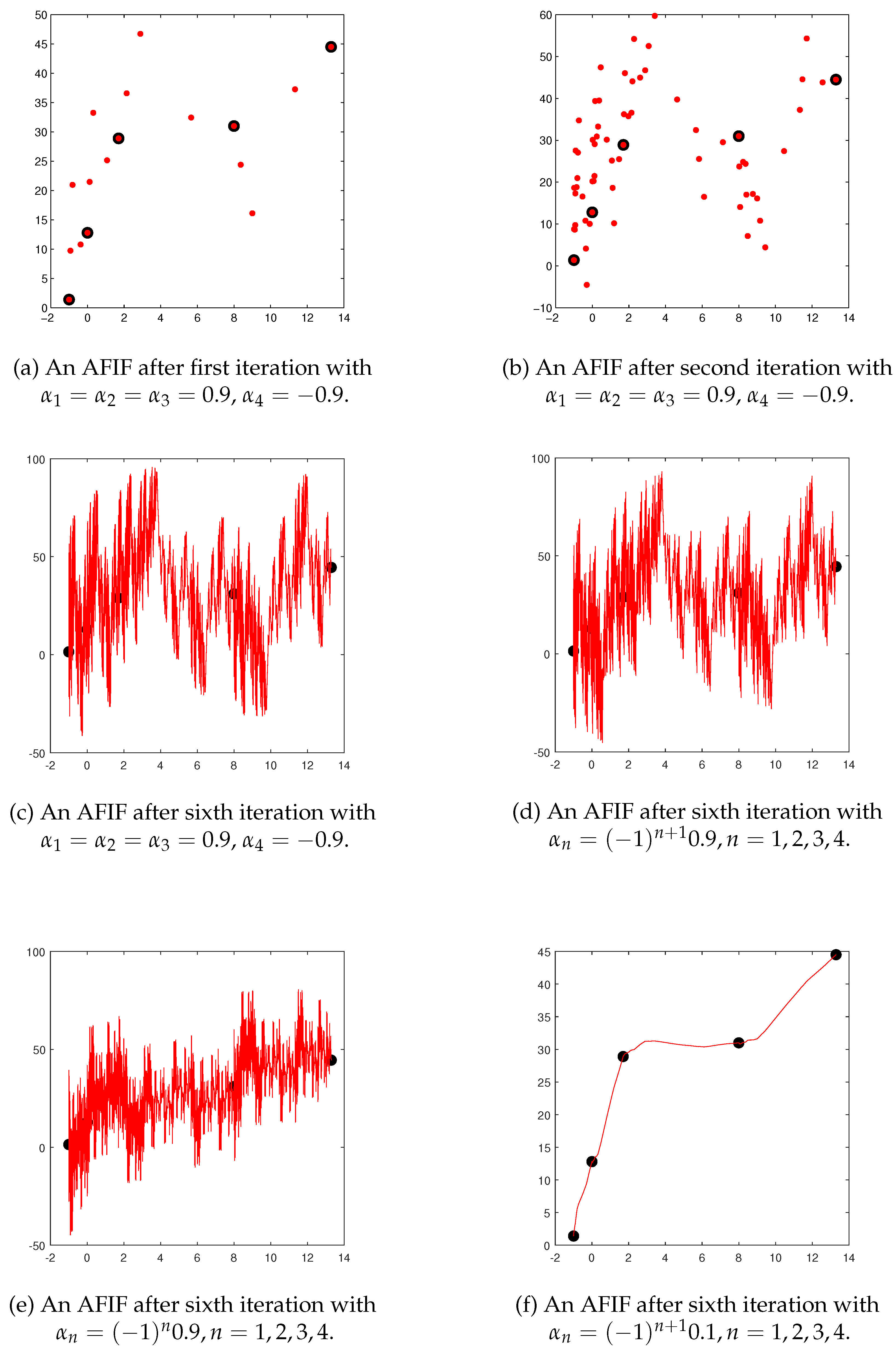
Example 1. 

Consider the interpolation data $\left\{\right(-1,1.4),(0,12.8),$$(1.7,28.9),$$(8,31),$$(13.3,$$44.5\left)\right\}$. From (7), it is clear that affine FIF is recursive. Hence, one has to use iterative procedure to evaluate the affine FIF at different points of $[-1,13.3]$. For the above data, after first, second, and sixth iteration, affine FIF with the scaling factors ${\alpha }_1={\alpha }_2={\alpha }_3=0.9,{\alpha }_4=-0.9$ is generated respectively in Figure 1a–c. From Figure 1a–c, it is clear that to obtain the values of affine FIF at more points of $[-1,13.3]$, one has to use more number of iterations. Similarly, some more affine FIFs are generated after sixth iteration in Figure 1d–f using different choices of the scaling factors as mentioned in the respective figure.

4.1. Inscribing Affine Fif in a Rectangle

In most of the applications, for instance fractal-based image encoding and compression, we need to interpolate the given data within a given rectangle. The sufficient conditions on the scaling factors which ensure that affine FIF sits within in the given rectangle are studied in [17,18]. The following proposition provides the details.

Proposition 2. 

Let $f_{\alpha }$ be an affine FIF associated with the data $\left\{(x_i,z_i),i\in {\mathbb{N}}_N^{*}\right\}$. Let $k_1<min\{z_i:i\in {\mathbb{N}}_N^{*}\}$ and $k_2>max\{z_i:i\in {\mathbb{N}}_N^{*}\}.$ Then graph of affine FIF $f_{\alpha }$ contained in the rectangle $[x_0,x_N]\times [k_1,k_2]$, if the scaling factors are chosen in the following way:

$$\begin{array}{c}\hfill {\alpha }_n\in ({\tau }_n^{*},{\tau }_n),n\in {\mathbb{N}}_N\end{array}$$

(9)

$$\begin{array}{cc}\hfill & where{\tau }_n=min\left\{1,\frac{z_{n-1}-k_1}{z_0-k_1},\frac{z_n-k_1}{z_N-k_1},\frac{k_2-z_{n-1}}{k_2-z_0},\frac{k_2-z_n}{k_2-z_N}\right\},\hfill \\ & {\tau }_n^{*}=max\left\{-1,\frac{-(z_{n-1}-k_1)}{k_2-z_0},\frac{-(z_n-k_1)}{k_2-z_N},\frac{-(k_2-z_{n-1})}{z_0-k_1},\frac{-(k_2-z_n)}{z_N-k_1}\right\}.\hfill \end{array}$$

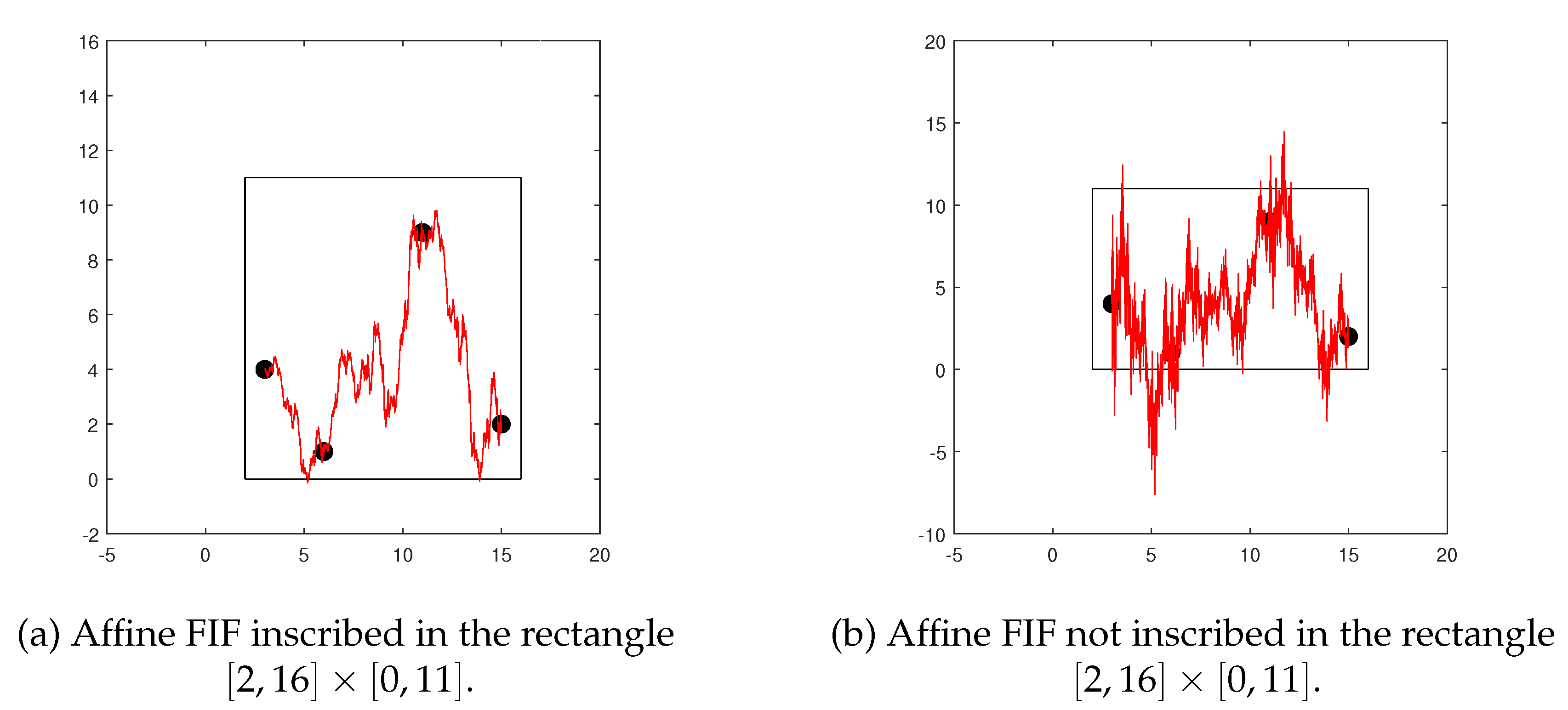
Example 2. 

We now illustrate the importance of Proposition 2 by constructing the examples of affine FIFs that interpolate the data set $\left\{\right(3,4),(6,1),(11,9),(15,2\left)\right\}$. Suppose that for some reason it is required to inscribe the graph of the interpolant in the rectangle $[2,16]\times [0,11].$ To obtain it, with respect to (9), the scaling vector is chosen as $\alpha =(-0.27,-0.6,-0.55,-0.5).$ The corresponding affine FIF inscribed in the rectangle $[2,16]\times [0,11]$ is generated in Figure 2a. Note in particular that the interpolating curve is non-negative, thus solving a constrained interpolation problem for the given data. Similarly, another affine FIF is generated in Figure 2b with the scaling vector $\alpha =(-0.8,-0.6,-0.6,-0.6)$. It is easy to verify that scaling vector $\alpha =(-0.8,-0.6,-0.6,-0.6)$ does not obey (9). As a result, the affine FIF generated in Figure 2b is not inscribed in the rectangle $[2,16]\times [0,11]$ and also affine FIF taking negative values although the given data is positive. From this experiment, we can understand imporatnce of (9) for obtaining the affine FIFs inscribed in the given rectangle.

4.2. Existence of Optimal Affine Fif

It can be easily seen from (6) that the affine FIF depends on the choice of the vertical scaling factors and there are infinite number of ways to select them. As a result, there exist an infinite number of affine FIFs corresponding to a given set of data. Hence, one can ask whether an optimal affine FIF exists. As an answer to this question, it is proved in [14] that there exists an affine FIF close to some classical interpolant f that interpolates the data points $(x_i,z_i),i\in {\mathbb{N}}_N^{*}$. Now, it is easy to verify that the affine FIF $f_{\alpha }$ is the fixed point of the Read-Bajraktarević operator $\left(T_{\alpha }h\right)\left(x\right)=g\left(x\right)+{\alpha }_n[h\left(x\right)-b\left(x\right)]\circ L_n^{-1}\left(x\right),x\in I_n,$ where g is the piecewise linear function that interpolates $(x_i,z_i),i\in {\mathbb{N}}_N^{*},$ and b is the line joining $(x_0,z_0)$ and $(x_N,z_N).$ Further, ${\left|\alpha \right|}_{\infty }$ is contractivity factor of $T_{\alpha }.$ Let us recall the Collage theorem [18,19] which serves as a prelude to our analysis.

Theorem 1 

(Collage Theorem). Let $f\in \mathcal{C}\left(I\right)$ and $U:\mathcal{C}\left(I\right)\to \mathcal{C}\left(I\right)$ be a contraction map with contractivity factor $c\in [0,1).$ If ${\parallel Uf-f\parallel }_{\infty }\le \epsilon ,$ then $\parallel f-\tilde{f}{\parallel }_{\infty }\le \frac{\epsilon }{1-c},$ where $\tilde{f}$ is fixed point of $U.$

The previous theorem states that, if $f\in \mathcal{C}\left(I\right)$ is given and ${\alpha }^{*}$ is such that $\parallel T_{{\alpha }^{*}}{f-f\parallel }_{\infty }\le \epsilon ,$ then

$$\parallel f-f_{{\alpha }^{*}}{\parallel }_{\infty }={\parallel f-T_{{\alpha }^{*}}{f}_{{\alpha }^{*}}\parallel }_{\infty }\le \frac{\epsilon }{1-|{\alpha }^{*}{|}_{\infty }}.$$

Owing to the above reason, we have to search for ${\alpha }^{*}\in \Sigma =\{\alpha \in {\mathbb{R}}^N{:\left|\alpha \right|}_{\infty }\le \mu <1\}$ such that $\parallel f-T_{{\alpha }^{*}}{f\parallel }_{\infty }$ is minimum.

Proposition 3. 

Let $f\in \mathcal{C}\left(I\right).$ Then the map $\eta :\Sigma \to \mathcal{C}\left(I\right)$ defined by $\eta \left(\alpha \right)=T_{\alpha }$ is Lipschitz continuous. Consequently, the map $F:\Sigma \to {\mathbb{R}}^{+}\cup \left\{0\right\}$ defined by $F\left(\alpha \right)=\parallel T_{\alpha }{f-f\parallel }_{\infty }$ is continuous.

Proof. 

Let $\alpha ,\beta \in \Sigma .$ From (4) and (5), we have

$$T_{\alpha }f=g\left(x\right)+{\alpha }_n\left[f\left(L_n^{-1}\left(x\right)\right)-b(L_n^{-1}\left(x\right)\right],x\in I_n,$$

$$T_{\beta }f=g\left(x\right)+{\beta }_n\left[f\left(L_n^{-1}\left(x\right)\right)-b(L_n^{-1}\left(x\right)\right],x\in I_n.$$

Consequently,

$$|T_{\alpha }f-T_{\beta }f|\le |{\alpha }_n-{\beta }_n{|\parallel f-b\parallel }_{\infty }.$$

Hence, we have

$$\parallel T_{\alpha }f-T_{\beta }{f\parallel }_{\infty }\le {|\alpha -\beta |}_{\infty }{\parallel f-b\parallel }_{\infty }{,|\alpha -\beta |}_{\infty }=max\left\{\right|{\alpha }_n-{\beta }_n|:n\in {\mathbb{N}}_N\}.$$

That is, ${\parallel \eta \left(\alpha \right)-\eta \left(\beta \right)\parallel }_{\infty }\le {|\alpha -\beta |}_{\infty }{\parallel f-b\parallel }_{\infty }.$ Therefore, $\eta$ is a Lipschitz continuous map with Lipschitz constant ${\parallel f-b\parallel }_{\infty }.$ Finally, continuity of F follows from the result that the sum and composition of continuous functions are continuous. □

Corollary 1. 

There exists an optimal scaling vector ${\alpha }^{*}\in \Sigma$ for which the function defined by $F\left(\alpha \right)=\parallel T_{\alpha }{f-f\parallel }_{\infty }$ is minimum.

Proof. 

Since the function $F:\Sigma \to {\mathbb{R}}^{+}\cup \left\{0\right\}$ is continuous and the set $\Sigma$ is compact, the existence of an optimal scaling vector ${\alpha }^{*}$ such that

$$F\left({\alpha }^{*}\right)=\underset{\alpha \in \Sigma }{min}F\left(\alpha \right)=\underset{\alpha \in \Sigma }{min}{\parallel T_{\alpha }f-f\parallel }_{\infty }$$

follows from the result that a continuous real function on a compact metric space attains its maximum and minimum. □

Having established the existence, now the following result provides a tool to find ${\alpha }^{*}.$

Proposition 4. 

The function $F:\Sigma \to {\mathbb{R}}^{+}\cup \left\{0\right\}$ defined by $F\left(\alpha \right)=\parallel T_{\alpha }{f-f\parallel }_{\infty }$ is convex.

Proof. 

Let $\alpha ,\beta \in \Sigma$ and $\lambda \in [0,1].$ It follows that

$$\begin{array}{cc}\hfill F\left(\right(1-\lambda )\alpha +\lambda \beta )=& max\left\{\right|T_{(1-\lambda )\alpha +\lambda \beta }f\left(x\right)-f\left(x\right)|:x\in I\}\hfill \\ \hfill =& \underset{n}{max}\underset{x\in I_n}{max}\left\{\right|[(1-\lambda ){\alpha }_n+\lambda {\beta }_n]\left[f\left(L_n^{-1}\left(x\right)\right)-b(L_n^{-1}\left(x\right)\right]+g\left(x\right)-b\left(x\right)\left|\right\}\hfill \\ \hfill \le & (1-\lambda )\underset{n}{max}\underset{x\in I_n}{max}\left\{\right|{\alpha }_n\left[f\left(L_n^{-1}\left(x\right)\right)-b(L_n^{-1}\left(x\right)\right]+g\left(x\right)-f\left(x\right)\left|\right\}\hfill \\ \hfill & +\lambda \underset{n}{max}\underset{x\in I_n}{max}\left\{\right|{\beta }_n\left[f\left(L_n^{-1}\left(x\right)\right)-b(L_n^{-1}\left(x\right)\right]+g\left(x\right)-f\left(x\right)\left|\right\}\hfill \\ \hfill =& (1-\lambda )\parallel T_{\alpha }{f-f\parallel }_{\infty }+\lambda {\parallel T_{\beta }f-f\parallel }_{\infty }\hfill \\ \hfill =& (1-\lambda )F\left(\alpha \right)+\lambda F\left(\beta \right).\hfill \end{array}$$

(10)

□

It is straight forward to see that $\Sigma$ is a convex subset of ${\mathbb{R}}^N.$ Consequently, from the previous proposition, it follows that the problem of finding ${\alpha }^{*}\in \Sigma$ such that $F\left({\alpha }^{*}\right)=\underset{\alpha \in \Sigma }{min}F\left(\alpha \right)$ is a constrained convex optimization problem. Following the Collage theorem, If ${\alpha }^{*}$ is the optimum scaling vector, then the expression $\frac{F\left({\alpha }^{*}\right)}{1-|{\alpha }^{*}{|}_{\infty }}$ provides an upper bound for the uniform distance $\parallel f-f_{{\alpha }^{*}}{\parallel }_{\infty },$ where f is a classical interpolant and $f_{{\alpha }^{*}}$ is the affine FIF close to f.

4.3. Convergence of Affine Fif

Theorem 2. 

(Navascués and Sebastián, 2007) Let $\psi \in \mathcal{C}\left(I\right)$. Let $f_{\alpha }$ be the affine FIF associated with the data set $\{(x_i,z_i)\in {\mathbb{R}}^2:i\in {\mathbb{N}}_N^{*}\},$ where $\psi \left(x_i\right)=z_i.$ Let g be the piecewise linear function that interpolates $(x_i,z_i),i\in {\mathbb{N}}_N^{*},$ that is, $g\left(x\right)=z_n\theta +z_{n-1}(1-\theta ),$ and $b\left(x\right)=z_N\theta +z_0(1-\theta ),\theta =\frac{x-x_{n-1}}{x_n-x_{n-1}},x\in I_n.$ Then

$$\parallel f_{\alpha }{-\psi \parallel }_{\infty }\le 2{\omega }_{\psi }\left(h\right)+\frac{{\left|\alpha \right|}_{\infty }}{1-{\left|\alpha \right|}_{\infty }}{\parallel g-b\parallel }_{\infty },$$

(11)

where ${\omega }_{\psi }\left(h\right)$ is the modulus of continuity of ψ defined by ${\omega }_{\psi }\left(h\right)={\displaystyle \underset{|x-x^{*}|\le h}{sup}}|\psi \left(x\right)-\psi \left(x^{*}\right)|$ and h is the norm of the partition defined by $h=max\{h_n:n\in {\mathbb{N}}_N\},$ where $h_n=x_n-x_{n-1}.$

Proof. 

We rewrite (7) in terms of g and b as

$$\begin{array}{cc}\hfill f_{\alpha }\left(x\right)-g\left(x\right)=& {\alpha }_n{f}_{\alpha }\left(L_n^{-1}\left(x\right)\right)-{\alpha }_{n}b\left(L_n^{-1}\left(x\right)\right),\hfill \\ \hfill =& {\alpha }_n\left[f_{\alpha }\left(L_n^{-1}\left(x\right)\right)-g\left(L_n^{-1}\left(x\right)\right)\right]+{\alpha }_{n}g\left(L_n^{-1}\left(x\right)\right)-{\alpha }_{n}b\left(L_n^{-1}\left(x\right)\right).\hfill \end{array}$$

Therefore, for $x\in I_n$,

$$\begin{array}{cc}\hfill |f_{\alpha }\left(x\right)-g\left(x\right)|\le & \left|{\alpha }_n\right||f_{\alpha }\left(L_n^{-1}\left(x\right)\right)-g\left(L_n^{-1}\left(x\right)\right)|+\left|{\alpha }_n\right|\left|g\left(L_n^{-1}\left(x\right)\right)\right|-b\left(L_n^{-1}\left(x\right)\right)|\hfill \\ \hfill \le & {\left|\alpha \right|}_{\infty }\parallel f_{\alpha }{-g\parallel }_{\infty }+{\left|\alpha \right|}_{\infty }{\parallel g-b\parallel }_{\infty }.\hfill \end{array}$$

Since the above inequality is valid for each $I_n$, $n\in {\mathbb{N}}_N,$ we have

$$\parallel f_{\alpha }{-g\parallel }_{\infty }\le {\left|\alpha \right|}_{\infty }\parallel f_{\alpha }{-g\parallel }_{\infty }+{\left|\alpha \right|}_{\infty }{\parallel g-b\parallel }_{\infty },$$

and hence

$$\parallel f_{\alpha }{-g\parallel }_{\infty }\le \frac{{\left|\alpha \right|}_{\infty }{\parallel g-b\parallel }_{\infty }}{1-{\left|\alpha \right|}_{\infty }}.$$

(12)

Noting that

$$\begin{array}{cc}\hfill g\left(x\right)-\psi \left(x\right)=& z_n\theta +z_{n-1}(1-\theta )-\psi \left(x\right)\hfill \\ \hfill =& (z_n-z_{n-1})\theta +z_{n-1}-\psi \left(x\right)\hfill \\ \hfill =& (z_n-z_{n-1})\theta +\psi \left(x_{n-1}\right)-\psi \left(x\right)\hfill \\ \hfill =& \left(\psi \left(x_n\right)-\psi \left(x_{n-1}\right)\right)\theta +\psi \left(x_{n-1}\right)-\psi \left(x\right).\hfill \end{array}$$

we find that

$${\parallel g-\psi \parallel }_{\infty }\le 2{\omega }_{\psi }\left(h\right).$$

(13)

Consider the triangle inequality

$$\parallel f_{\alpha }{-\psi \parallel }_{\infty }\le \parallel f_{\alpha }{-g\parallel }_{\infty }+{\parallel g-\psi \parallel }_{\infty }.$$

(14)

Combining (13) and (12) with (14), we settle (11). □

Since $\psi \in \mathcal{C}\left(I\right)$ is uniformly continuous, ${\omega }_{\psi }\left(h\right)\to 0$ as $h\to 0$. Therefore, from Theorem 2, we assert that $f_{\alpha }$ converges to $\psi$ as $h\to 0$ and ${\left|\alpha \right|}_{\infty }\to 0.$

5. Bernstein Affine Fif

Let the data set $\{(x_i,z_i)\in {\mathbb{R}}^2:i\in {\mathbb{N}}_N\}$ be obtained from the function $\psi \in \mathcal{C}[x_1,x_N].$ Let $h=max\{h_i:i\in {\mathbb{N}}_{N-1}\},$ where $h_i=x_{i+1}-x_i.$ Let g be the piecewise linear function that interpolates $(x_i,z_i),i\in {\mathbb{N}}_N,$ that is, $g\left(x\right)=z_{i+1}\theta +z_i(1-\theta ),\theta =\frac{x-x_i}{x_{i+1}-x_i},x\in I_i.$ In the previous section (Theorem 2), it is seen that the affine FIF $f_{\alpha }$ associated with the data set $\{(x_i,z_i)\in {\mathbb{R}}^2:i\in {\mathbb{N}}_N\}$ converges to the data generating function if $h\to 0$ and ${\left|\alpha \right|}_{\infty }\to 0.$ In the present section, we develop a sequence of Bernstein affine FIFs corresponding the data set $\{(x_i,z_i)\in {\mathbb{R}}^2:i\in {\mathbb{N}}_N\}$ that converges uniformly to $\psi$ if $h\to 0.$ In (3), we choose the $q_i$ as

$$q_i\left(x\right)=g\left(L_i\left(x\right)\right)-{\alpha }_i{B}_n(g,x),$$

where $B_n(g,x)$ is the Bernstein polynomial [20] of g, i.e.,

$$B_n(g,x)=\frac{1}{{(x_N-x_1)}^n}\sum _{k=0}^n\left(\begin{array}{c}n\\ k\end{array}\right){(x-x_1)}^k{(x_N-x)}^{n-k}g\left(x_1+\frac{k(x_N-x_1)}{n}\right),\forall x\in I,\forall n\in \mathbb{N}.$$

It is easy to verify that $B_n(g,x_1)=g\left(x_1\right)$, $B_n(g,x_N)=g\left(x_N\right)$ for all $n\in \mathbb{N}.$ In this case, the affine FIF $f_{\alpha }$= $f_{n,\alpha },n\in \mathbb{N}$ is called the Bernstein affine FIF corresponding to $\{(x_i,z_i)\in {\mathbb{R}}^2:i\in {\mathbb{N}}_N\}$ and

$$f_{n,\alpha }\left(x\right)={\alpha }_i{f}_{n,\alpha }\left(L_i^{-1}\left(x\right)\right)+g\left(x\right)-{\alpha }_i{B}_n(g,L_i^{-1}\left(x\right)),x\in I_i,i\in {\mathbb{N}}_{N-1}.$$

(15)

From the construction of fractal functions (see previous section), it can be verified that for every $n\in \mathbb{N},$ the Bernstein affine FIF $f_{n,\alpha }$ is obtained via the IFS defined by

$${\mathcal{I}}_n=\{I\times K,\left(L_i\left(x\right),F_{n,i}(x,z)\right),i\in {\mathbb{N}}_{N-1}\},$$

(16)

where $F_{n,i}(x,z)={\alpha }_{i}z+g\left(L_i\left(x\right)\right)-{\alpha }_i{B}_n(g,x).$ From (15), it is easy to notice that for a given $f\in \mathcal{C}\left(I\right)$ there exists a sequence ${\left\{f_{n,\alpha }\right\}}_{n=1}^{\infty }$ of Bernstein affine FIFs. The following theorem addresses the convergence of the sequence ${\left\{f_{n,\alpha }\right\}}_{n=1}^{\infty }$ towards the data generating function $\psi \in \mathcal{C}\left(I\right).$

Theorem 3. 

Let $\psi \in \mathcal{C}\left(I\right)$. Let $\{(x_i,z_i)\in {\mathbb{R}}^2:i\in {\mathbb{N}}_N\}$ be a data set, where $\psi \left(x_i\right)=z_i.$ Let $g\left(x\right)=z_{i+1}\theta +z_i(1-\theta ),\theta =\frac{x-x_i}{x_{i+1}-x_i},x\in I_i.$ Let $\alpha =({\alpha }_1,{\alpha }_2,\cdots ,{\alpha }_{N-1}).$ Then, for every scaling vector $\alpha ,$ the sequence ${\left\{{\mathcal{I}}_n\right\}}_{n=1}^{\infty }$ of IFSs determine a sequence ${\left\{f_{n,\alpha }\right\}}_{n=1}^{\infty }$ of Bernstein affine FIFs that converges uniformly to the data generating function $\psi .$

Proof. 

From (15), it is easy to deduce that

$$\begin{array}{cc}\hfill \parallel f_{n,\alpha }{-g\parallel }_{\infty }\le & {\left|\alpha \right|}_{\infty }{\parallel f_{n,\alpha }-B_n(g,.)\parallel }_{\infty },\hfill \\ \hfill \le & {\left|\alpha \right|}_{\infty }[\parallel f_{n,\alpha }{-g\parallel }_{\infty }+\parallel g-B_n(g,.){\parallel }_{\infty }].\hfill \end{array}$$

Hence we obtain

$$\begin{array}{c}\hfill \parallel f_{n,\alpha }{-g\parallel }_{\infty }\le \frac{{\left|\alpha \right|}_{\infty }}{1-{\left|\alpha \right|}_{\infty }}{\parallel g-B_n(g,.)\parallel }_{\infty }.\end{array}$$

(17)

Substituting (13) and (17) in (14), we get

$$\parallel f_{n,\alpha }{-\psi \parallel }_{\infty }\le 2{\omega }_{\psi }\left(h\right)+\frac{{\left|\alpha \right|}_{\infty }}{1-{\left|\alpha \right|}_{\infty }}{\parallel g-B_n(g,.)\parallel }_{\infty },$$

(18)

where ${\omega }_{\psi }\left(h\right)$ is the modulus of continuity of $\psi .$ Since $\psi \in \mathcal{C}\left(I\right)$ is uniformly continuous, ${\omega }_{\psi }\left(h\right)\to 0$ as $h\to 0$ and from the approximation theory [20], it follows that $\parallel g-B_n{(g,.)\parallel }_{\infty }\to 0$ and $n\to \infty .$ As a result, from (18), it follows that $f_{n,\alpha }\to \psi$ uniformly if $h\to 0$ and $n\to \infty .$ □

6. Bernstein Affine Fis

Let us consider the surface data set placed on the rectangular grid $D_{\mathrm{grid}}:x_1<x_2<\cdots <x_{N-1}<x_N,$$y_1<y_2<\cdots <y_{M-1}<y_M,$ be given by ${▵}_1=\{(x_i,y_j,z_{i,j})\in {\mathbb{R}}^3$|$i\in {\mathbb{N}}_N,j\in {\mathbb{N}}_M\}.$ Let $I=[x_1,x_N]$, $I_i=[x_i,x_{i+1}]$, $J=[y_1,y_M]$, $J_j=[y_j,y_{j+1}]$, and $D=I\times J$, and $D_{i,j}=I_i\times J_j$. We construct the Bernstein affine fractal surface ${\mathsf{\Phi }}_n,n\in \mathbb{N}$ as a blending of the Bernstein affine FIFs constructed along the grid lines of the interpolation domain D so that ${\mathsf{\Phi }}_n:D\to \mathbb{R}$, ${\mathsf{\Phi }}_n(x_i,y_j)=z_{i,j}$, $i\in {\mathbb{N}}_N,j\in {\mathbb{N}}_M$. Now for above surface data, $T_j=\{(x_i,z_{i,j}):i\in {\mathbb{N}}_N\}$ is the interpolation data along the $j\mathrm{th},j\in {\mathbb{N}}_M$ grid line parallel to x-axis. Similarly, $T_i^{*}=\{(y_j,z_{i,j}):j\in {\mathbb{N}}_M\}$ is the interpolation data along the $i\mathrm{th},i\in {\mathbb{N}}_N$ grid line parallel to y-axis. For $j\in {\mathbb{N}}_M,$ let $g_j\left(x\right)=z_{i+1,j}\theta +z_{i,j}(1-\theta ),\theta =\frac{x-x_i}{x_{i+1}-x_i},x\in I_i.$ Similarly, for $i\in {\mathbb{N}}_N,$ let $g_i^{*}\left(y\right)=z_{i,j+1}\varphi +z_{i,j}(1-\varphi ),\varphi =\frac{y-y_j}{y_{j+1}-y_j},y\in J_j.$ Suppose ${\mathsf{\Psi }}_{n,j}(x,{\alpha }_{i,j})$ and ${\mathsf{\Psi }}_{n,i}^{*}(y,{\alpha }_{i,j}^{*})$ are the Bernstein affine FIFs interpolating the data sets $T_j$ and $T_i^{*}$ respectively. By utilizing the functional equation of the Bernstein affine FIF $f_{n,\alpha }$ (cf. (15)), we obtain the functional equations of ${\mathsf{\Psi }}_{n,j}(x,{\alpha }_{i,j}),$$j\in {\mathbb{N}}_M$ and ${\mathsf{\Psi }}_{n,i}^{*}(y,{\alpha }_{i,j}^{*}),$$i\in {\mathbb{N}}_N$ respectively as

$${\mathsf{\Psi }}_{n,j}(x,{\alpha }_{i,j})={\alpha }_{i,j}{\mathsf{\Psi }}_{n,j}(L_i^{-1}\left(x\right),{\alpha }_{i,j})+g_j\left(x\right)-{\alpha }_{i,j}{B}_n(g_j,L_i^{-1}\left(x\right)),\theta =\frac{L_i^{-1}\left(x\right)-x_1}{x_N-x_1},x\in I_i,$$

(19)

$${\mathsf{\Psi }}_{n,i}^{*}(y,{\alpha }_{i,j}^{*})={\alpha }_{i,j}^{*}{\mathsf{\Psi }}_{n,i}^{*}(L_j^{*-1}\left(y\right),{\alpha }_{i,j}^{*})++g_i^{*}\left(y\right)-{\alpha }_{i,j}^{*}{B}_n(g_i^{*},L_j^{*-1}\left(y\right)),\varphi =\frac{L_j^{*-1}\left(y\right)-y_1}{y_M-y_1},y\in J_j,$$

(20)

${\alpha }_{i,j}$ and ${\alpha }_{i,j}^{*}$ are the scaling factors in x-direction and y-direction respectively satisfying $|{\alpha }_{i,j}|<1$ and $|{\alpha }_{i,j}^{*}|<1,$$L_j^{*}\left(y\right)=c_{j}y+d_j=\frac{(y_{j+1}-y_j)y}{y_N-y_1}+\frac{y_M{y}_j-y_1{y}_{j+1}}{y_M-y_1}:J\to J_j$ is a homeomorphism such that $L_j^{*}\left(y_1\right)=y_j,L_j^{*}\left(y_M\right)=y_{j+1},j\in {\mathbb{N}}_{M-1}$. Now we define the Bernstein affine FIS ${\mathsf{\Phi }}_n$ as blending of the above affine FIFs ${\mathsf{\Psi }}_{n,j},j\in {\mathbb{N}}_M$ and ${\mathsf{\Psi }}_{n,i}^{*},$$i\in {\mathbb{N}}_N$. In the present construction, we use the following choice of blending functions:

$a_{x,0}\left(\theta \right)={(1-\theta )}^2(1+2\theta ),$$a_{x,1}\left(\theta \right)={\theta }^2(3-2\theta )$, $\theta =\frac{L_i^{-1}\left(x\right)-x_1}{x_N-x_1}=\frac{x-x_i}{x_{i+1}-x_i},$$x\in I_i,$

$b_{y,0}\left(\varphi \right)={(1-\varphi )}^2(1+2\varphi )$, $b_{y,1}\left(\varphi \right)={\varphi }^2(3-2\varphi )$, $\varphi =\frac{L_j^{*-1}\left(y\right)-y_1}{y_M-y_1}=\frac{y-y_j}{y_{j+1}-y_j},$$y\in J_j.$

The boundary of the sub-rectangle $D_{i,j}$ is taken as the union of four boundary lines $I_i\times y_j,$$I_i\times y_{j+1},$$x_i\times J_j,$ and $x_{i+1}\times J_j$. We define ${\mathsf{\Phi }}_n,n\in \mathbb{N}$ over $D_{i,j},$$i\in {\mathbb{N}}_{N-1},$$j\in {\mathbb{N}}_{M-1},$ as

$${\mathsf{\Phi }}_n(x,y)=-M_1{{\rm Y}}_n(x,y)M_2^T,(x,y)\in D_{i,j},$$

(21)

$$\mathrm{where}{{\rm Y}}_n(x,y)=\left[\begin{array}{ccc}0& {\mathsf{\Psi }}_{n,j}(x,{\alpha }_{i,j})& {\mathsf{\Psi }}_{n,j+1}(x,{\alpha }_{i,j+1})\\ {\mathsf{\Psi }}_{n,i}^{*}(y,{\alpha }_{i,j}^{*})& z_{i,j}& z_{i,j+1}\\ {\mathsf{\Psi }}_{n,i+1}^{*}(y,{\alpha }_{i+1,j}^{*})& z_{i+1,j}& z_{i+1,j+1}\end{array}\right],M_1=[-1a_{x,0}\left(\theta \right)a_{x,1}\left(\theta \right)],$$

and $M_2=[-1b_{y,0}\left(\varphi \right)b_{y,1}\left(\varphi \right)]$. From (21), it easy to verify that ${\mathsf{\Phi }}_n(x_i,y_j)=z_{i,j}$, ${\mathsf{\Phi }}_n(x_{i+1},y_j)=z_{i+1,j}$, ${\mathsf{\Phi }}_n(x_i,y_{j+1})=z_{i,j+1}$, ${\mathsf{\Phi }}_n(x_{i+1},y_{j+1})=z_{i+1,j+1}$, $i\in {\mathbb{N}}_{N-1}$, $j\in {\mathbb{N}}_{M-1}.$ Thus ${\mathsf{\Phi }}_n$ interpolates ${▵}_1$ at the grid points of the interpolation domain D. We invite the readers to check that ${\mathsf{\Phi }}_n(x_i,y)={\mathsf{\Psi }}_{n,i}^{*}(y,{\alpha }_{i,j}^{*}),{\mathsf{\Phi }}_n(x_{i+1},y)={\mathsf{\Psi }}_{n,i+1}^{*}(y,{\alpha }_{i+1,j}^{*}),{\mathsf{\Phi }}_n(x,y_j)={\mathsf{\Psi }}_j(x,{\alpha }_{i,j}),{\mathsf{\Phi }}_n(x,y_{j+1})$$={\mathsf{\Psi }}_{n,j+1}(x,{\alpha }_{i,j+1})$. In other words, along the boundaries $I_i\times y_j$,$I_i\times y_{j+1}$, $x_i\times J_j$, and $x_{i+1}\times J_j$ of $D_{i,j}$, the fractal surface ${\mathsf{\Phi }}_n$ reduces to Bernstein affine FIFs ${\mathsf{\Psi }}_{n,j}(x,{\alpha }_{i,j})$, ${\mathsf{\Psi }}_{n,j+1}(x,{\alpha }_{i,j+1})$, ${\mathsf{\Psi }}_{n,i}^{*}(y,{\alpha }_{i,j}^{*})$, and ${\mathsf{\Psi }}_{n,i+1}^{*}(y,{\alpha }_{i+1,j}^{*})$ respectively. Similarly, using (21), the fractal surface ${\mathsf{\Phi }}_n$ over the sub-rectangle $D_{i,j+1}$ is defined as a blending of the Bernstein affine FIFs ${\mathsf{\Psi }}_{n,j+1}(x,{\alpha }_{i,j+1})$, ${\mathsf{\Psi }}_{n,j+2}(x,{\alpha }_{i,j+2})$, ${\mathsf{\Psi }}_{n,i}^{*}(y,{\alpha }_{i,j+1}^{*}),$$y\in J_{j+1}$, and ${\mathsf{\Psi }}_{n,i+1}^{*}(y,{\alpha }_{i+1,j+1}^{*}),$$y\in J_{j+1}$. Along the boundary line $I_i\times J_{j+1}$, the fractal surface ${\mathsf{\Phi }}_n$ reduces to ${\mathsf{\Psi }}_{n,j+1}(x,{\alpha }_{i,j+1})$, and hence ${\mathsf{\Phi }}_n$ is continuous over the the domains $D_{i,j}\cup D_{i,j+1},$$i\in {\mathbb{N}}_{N-1},$$j\in {\mathbb{N}}_{M-2}$. A similar type of arguments gives that ${\mathsf{\Phi }}_n$ is continuous over the the domain $D_{i,j}\cup D_{i+1,j},$$i\in {\mathbb{N}}_{N-2},$$j\in {\mathbb{N}}_{M-1}$. From the above discussion, we conclude that the fractal surface ${\mathsf{\Phi }}_n$ is continuous over the interpolation domain D. Since we have used only Bernstein affine FIFs in the construction of ${\mathsf{\Phi }}_n$, we refer it as Bernstein affine FIS. The scaling factors involved in the Bernstein affine FIFs ${\mathsf{\Psi }}_{n,j},$$j\in {\mathbb{N}}_M$, and ${\mathsf{\Psi }}_{n,i}^{*}$, $i\in {\mathbb{N}}_N$ are put in matrices $\alpha ={\left[{\alpha }_{i,j}\right]}_{(N-1)\times M}$, and ${\alpha }^{*}={\left[{\alpha }_{i,j}^{*}\right]}_{N\times (M-1)}$ respectively.

Remark 2. 

If $\alpha ={\left[0\right]}_{(N-1)\times M}$ and ${\alpha }^{*}={\left[0\right]}_{N\times (M-1)}$, then we get the classical affine surface interpolant as

$$\begin{array}{cc}\hfill S_n(x,y)=& b_{y,0}\left(\varphi \right){\mathsf{\Psi }}_{n,j}(x,0)+b_{y,1}\left(\varphi \right){\mathsf{\Psi }}_{n,j+1}(x,0)+a_{x,0}\left(\theta \right){\mathsf{\Psi }}_{n,i}^{*}(y,0)\hfill \\ & +a_{x,1}\left(\theta \right){\mathsf{\Psi }}_{n,i+1}^{*}(y,0)-a_{x,0}\left(\theta \right)b_{y,0}\left(\varphi \right)z_{i,j}-a_{x,0}\left(\theta \right)b_{y,1}\left(\varphi \right)z_{i,j+1}\hfill \\ & -a_{x,1}\left(\theta \right)b_{y,0}\left(\varphi \right)z_{i+1,j}-a_{x,1}\left(\theta \right)b_{y,1}\left(\varphi \right)z_{i+1,j+1},\hfill \end{array}$$

(22)

where ${\mathsf{\Psi }}_{n,j}(x,0)=g_j\left(x\right)$ and ${\mathsf{\Psi }}_{n,i}^{*}(y,0)=g_i^{*}\left(y\right)$ are the classical affine interpolants for the data sets $T_j$ and $T_i^{*}$ respectively.

Convergence of Bernstein affine FIS

Theorem 4. 

For $n\in \mathbb{N},$ let ${\mathsf{\Phi }}_n$ be the Bernstein affine FIS with respect to the surface data $\{(x_i,y_j,z_{i,j}):i\in {\mathbb{N}}_N,j\in {\mathbb{N}}_M\}$ generated from the function $F\in \mathcal{C}\left(D\right)$. Then, the sequence ${\left\{{\mathsf{\Phi }}_n\right\}}_{n=1}^{\infty }$ of Bernstein affine FISs converges uniformly to $F\in \mathcal{C}\left(D\right)$ if $h\to 0$ and $k\to 0,$ where $h=max\{x_{i+1}-x_i:i\in {\mathbb{N}}_{N-1}\}$ and $k=max\{y_{j+1}-y_j:j\in {\mathbb{N}}_{M-1}\}.$

Proof. 

From (21) and Remark 2, we have

$$\begin{array}{cc}\hfill |{\mathsf{\Phi }}_n(x,y)-S_n(x,y)|\le & b_{y,0}\left(\varphi \right)|{\mathsf{\Psi }}_{n,j}(x,{\alpha }_{i,j})-{\mathsf{\Psi }}_{n,j}(x,0)|\hfill \\ & +b_{y,1}\left(\varphi \right)|{\mathsf{\Psi }}_{n,j+1}(x,{\alpha }_{i,j+1})-{\mathsf{\Psi }}_{n,j+1}(x,0)|\hfill \\ & +a_{x,0}\left(\theta \right)|{\mathsf{\Psi }}_{n,i}^{*}(y,{\alpha }_{i,j}^{*})-{\mathsf{\Psi }}_{n,i}^{*}(y,0)|\hfill \\ & +a_{x,1}\left(\theta \right)|{\mathsf{\Psi }}_{n,i+1}^{*}(y,{\alpha }_{i,j}^{*})-{\mathsf{\Psi }}_{n,i+1}^{*}(y,0)|.\hfill \end{array}$$

(23)

Since ${\mathsf{\Psi }}_{n,j}(x,0)=g_j\left(x\right)$ and ${\mathsf{\Psi }}_{n,i}^{*}(y,0)=g_i^{*}\left(y\right),$ using (17), we obtain

$$\begin{array}{cc}\hfill & |{\mathsf{\Psi }}_{n,j}(x,{\alpha }_{i,j})-{\mathsf{\Psi }}_{n,j}(x,0)|\le \frac{|{\alpha }_j{|}_{\infty }}{1-|{\alpha }_j{|}_{\infty }}{\parallel g_j-B_n(g_j,.)\parallel }_{\infty },j\in {\mathbb{N}}_M,\hfill \\ & {\mathsf{\Psi }}_{n,i}^{*}(y,{\alpha }_{i,j}^{*})-{\mathsf{\Psi }}_{n,i}^{*}(y,0)|\le \frac{|{\alpha }_i^{*}{|}_{\infty }}{1-|{\alpha }_i^{*}{|}_{\infty }}{\parallel g_i^{*}-B_n(g_i^{*},.)\parallel }_{\infty },i\in {\mathbb{N}}_N,\hfill \end{array}$$

(24)

$|{\alpha }_j{|}_{\infty }=max\left\{\right|{\alpha }_{i,j}|:i\in {\mathbb{N}}_{N-1}\},$ and $|{\alpha }_i^{*}{|}_{\infty }=max\left\{\right|{\alpha }_{i,j}^{*}|:j\in {\mathbb{N}}_{M-1}\}.$ Also it is easy to calculate that

$$a_{x,0}\le 1,a_{x,1}\le 1,b_{y,0}\le 1,b_{y,1}\le 1.$$

(25)

$$\begin{array}{cc}\hfill |{\mathsf{\Phi }}_n(x,y)-S_n(x,y)|\le & \frac{|{\alpha }_j{|}_{\infty }}{1-|{\alpha }_j{|}_{\infty }}{\parallel g_j-B_n(g_j,.)\parallel }_{\infty }\hfill \\ & +\frac{|{\alpha }_{j+1}{|}_{\infty }}{1-|{\alpha }_{j+1}{|}_{\infty }}{\parallel g_{j+1}-B_n(g_{j+1},.)\parallel }_{\infty }\hfill \\ & +\frac{|{\alpha }_i^{*}{|}_{\infty }}{1-|{\alpha }_i^{*}{|}_{\infty }}{\parallel g_i^{*}-B_n(g_i^{*},.)\parallel }_{\infty }\hfill \\ & +\frac{|{\alpha }_{i+1}^{*}{|}_{\infty }}{1-|{\alpha }_{i+1}^{*}{|}_{\infty }}{\parallel g_{i+1}^{*}-B_n(g_{i+1}^{*},.)\parallel }_{\infty }.\hfill \end{array}$$

(26)

Since the above inequality is true for every $(x,y)\in D_{i,j},i\in {\mathbb{N}}_{N-1},j\in {\mathbb{N}}_{M-1},$ we get

$$\begin{array}{cc}\hfill \parallel {\mathsf{\Phi }}_n-S_n{\parallel }_{\infty }\le & \frac{|{\alpha }_j{|}_{\infty }}{1-|{\alpha }_j{|}_{\infty }}{\parallel g_j-B_n(g_j,.)\parallel }_{\infty }\hfill \\ & +\frac{|{\alpha }_{j+1}{|}_{\infty }}{1-|{\alpha }_{j+1}{|}_{\infty }}{\parallel g_{j+1}-B_n(g_{j+1},.)\parallel }_{\infty }\hfill \\ & +\frac{|{\alpha }_i^{*}{|}_{\infty }}{1-|{\alpha }_i^{*}{|}_{\infty }}{\parallel g_i^{*}-B_n(g_i^{*},.)\parallel }_{\infty }\hfill \\ & +\frac{|{\alpha }_{i+1}^{*}{|}_{\infty }}{1-|{\alpha }_{i+1}^{*}{|}_{\infty }}{\parallel g_{i+1}^{*}-B_n(g_{i+1}^{*},.)\parallel }_{\infty }.\hfill \end{array}$$

(27)

Applying the procedure which is similar to the procedure used in obtaining (13), we get

$$\parallel F-S_n\parallel \le e({\omega }_{F_j\left(h\right)}+{\omega }_{F_i\left(k\right)}),$$

(28)

where e is a suitable constant, ${\omega }_{F_j\left(h\right)}$ is the modulus of continuity of $F(x,y_j),$ and ${\omega }_{F_i\left(k\right)}$ is the modulus of continuity of $F(x_i,y).$

Consider the triangle inequality

$$\parallel {\mathsf{\Phi }}_n{-F\parallel }_{\infty }\le \parallel {\mathsf{\Phi }}_n-S_n{\parallel }_{\infty }+{\parallel S_n-F\parallel }_{\infty }.$$

(29)

Combining (27) and (28) with (29), we obtain

$$\begin{array}{cc}\hfill \parallel {\mathsf{\Phi }}_n{-F\parallel }_{\infty }\le & \frac{|{\alpha }_j{|}_{\infty }}{1-|{\alpha }_j{|}_{\infty }}{\parallel g_j-B_n(g_j,.)\parallel }_{\infty }\hfill \\ & +\frac{|{\alpha }_{j+1}{|}_{\infty }}{1-|{\alpha }_{j+1}{|}_{\infty }}{\parallel g_{j+1}-B_n(g_{j+1},.)\parallel }_{\infty }\hfill \\ & +\frac{|{\alpha }_i^{*}{|}_{\infty }}{1-|{\alpha }_i^{*}{|}_{\infty }}{\parallel g_i^{*}-B_n(g_i^{*},.)\parallel }_{\infty }\hfill \\ & +\frac{|{\alpha }_{i+1}^{*}{|}_{\infty }}{1-|{\alpha }_{i+1}^{*}{|}_{\infty }}{\parallel g_{i+1}^{*}-B_n(g_{i+1}^{*},.)\parallel }_{\infty }+e({\omega }_{F_j\left(h\right)}+{\omega }_{F_i\left(k\right)}).\hfill \end{array}$$

(30)

Now, it is easy to verify that (i) $\parallel g_j-B_n(g_j,.){\parallel }_{\infty }\to 0,j\in {\mathbb{N}}_M$ and $\parallel g_i^{*}-B_n(g_i^{*},.){\parallel }_{\infty }\to 0,i\in {\mathbb{N}}_N$ as $n\to \infty$, (ii) ${\omega }_{F_j\left(h\right)}\to 0,j\in {\mathbb{N}}_M$ and ${\omega }_{F_i\left(k\right)}\to 0,i\in {\mathbb{N}}_N,$ as $h,k\to 0.$ Consequently, we get the desired result from (30). □

Example 3. 

The Bernstein affine FISs ${\mathsf{\Phi }}_1$ and ${\mathsf{\Phi }}_{26}$ in Figure 3a,b are constructed with respect to the surface data given in

Table 1. Surface data.

$\downarrow \mathit{y}/\mathit{x}\to$	−4	−3	−2	−1
0.1	2	12	9	7
0.2	7	3	1	2
0.3	8	3	9	8
0.8	2	3	6	9

and the scaling matrices $\alpha ={\left[0.99\right]}_{3\times 4}$ and ${\alpha }^{*}={[-0.99]}_{4\times 3}$.

7. Discussion

If the magnitude of the scaling factors goes to zero, then the corresponding existing affine FIFs converge to the data generating function. In this case, the scaling factors may not fulfil condition (8). Consequently, the box-counting dimension of the existing affine FIFs would be one. In this article, using the Bernstein polynomials and the theory of IFSs, we have presented Bernstein affine FIFs as a comprehensive tool to analyse the data that originated from an irregular phenomenon. In our approach, the convergence of Bernstein FIFs towards the original function does not demand any condition on the scaling factors. As a result, we can fulfil the condition (8) and the box-counting dimension of the Bernstein affine FIFs must lie between one and two. In this work, we have also introduced the Bernstein affine FIS for the data arranged on the rectangular grid. The convergence of the affine FISs studied in [21] demand a condition on the scaling factors whereas our Bernstein affine FIS does not need any such condition. Because the shapes of the Bernstein affine FISs can be adjusted by using different choices of the scaling factors, our scheme offers a large flexibility for simulation or modelling of irregular objects. The optimal approximation of the Bernstein affine FIS for a given surface is under investigation using a genetic algorithm.

8. Materials and Methods

In the present article, we have used a sequential approach for obtaining a new class of affine FIFs, namely, Bernstein affine FIFs. Owing to the sequential technique, the convergence of the proposed Bernstein affine FIFs or FISs does depend on the choice of the scaling factors. A three dimensional problem can be approximated by either a two-dimensional or one-dimensional case, but some information will be lost. Two-scale mathematics is needed in order to reveal the lost information due to the lower dimensional approach. Generally, one scale is established by usage where traditional calculus works, and the other scale is for revealing the lost information where the continuum assumption might be forbidden, and fractional calculus or fractal calculus has to be used. Additionally, we have exploited the blending technique [22] for the construction of Bernstein affine FISs.

References

- Hutchinson, J.E. Fractals and self similarity. Indiana Univ. Math. J. 1981, 30, 713–747. [Google Scholar] [CrossRef]
- Barnsley, M.F. Fractal functions and interpolation. Constr. Approx. 1986, 2, 303–329. [Google Scholar] [CrossRef]
- Barnsley, M.F. Fractals Everywhere, 3rd ed.; Dover Publications, Inc.: New York, NY, USA, 2012. [Google Scholar]
- Maragos, P. Fractal aspects of speech signals: Dimension and interpolation. In Proceedings of the ICASSP 91: 1991 International Conference on Acoustics, Speech, and Signal Processing, Toronto, ON, Canada, 14–17 April 1991; Volume 1, pp. 417–420. [Google Scholar]
- Chand, A.K.B.; Kapoor, G.P. Generalized cubic spline fractal interpolation functions. SIAM J. Numer. Anal. 2006, 44, 655–676. [Google Scholar] [CrossRef] [Green Version]
- Viswanathan, P.; Chand, A.K.B.; Navascués, M.A. Fractal perturbation preserving fundamental shapes: Bounds on the scale factors. J. Math. Anal. Appl. 2014, 419, 804–817. [Google Scholar] [CrossRef]
- Vijender, N. Bernstein fractal trigonometric approximation. Acta Appl. Math. 2018, 159, 11–27. [Google Scholar] [CrossRef]
- Ali, M.; Clarkson, T.G. Using linear fractal interpolation functions to compress video images. Fractals 1994, 2, 417–421. [Google Scholar] [CrossRef]
- Barnsley, M.F. Fractal image compression. Not. Am. Math. Soc. 1996, 43, 657–662. [Google Scholar]
- Craciunescu, O.I.; Das, S.K.; Poulson, J.M.; Samulski, T.V. Three dimensional tumor perfusion reconstruction using fractal interpolation functions. IEEE Trans. Biomed. Eng. 2001, 48, 462–473. [Google Scholar] [CrossRef] [PubMed]
- Mazel, D.S.; Hayes, M.H. Using iterated function systems to model discrete sequences. IEEE Trans. Signal Process. 1992, 40, 1724–1734. [Google Scholar] [CrossRef]
- Dillon, S.; Drakopoulos, V. On Self-Affine and Self-Similar Graphs of Fractal Interpolation Functions Generated from Iterated Function Systems. In Fractal Analysis: Applications in Health Sciences and Social Sciences; Brambila, F., Ed.; Intech: Rijeka, Croatia, 2017; Chapter 9; pp. 187–205. [Google Scholar] [CrossRef] [Green Version]
- Ri, S.; Drakopoulos, V. How are fractal interpolation functions related to several contractions? In Mathematical Theorems; Alexeyeva, L., Ed.; Intech: Rijeka, Croatia, 2020. [Google Scholar]
- Navascués, M.A.; Sebastián, M.V. Construction of affine fractal functions close to classical interpolants. J. Comput. Anal. Appl. 2007, 9, 271–285. [Google Scholar]
- Navascués, M.A. Fractal approximation. Complex Anal. Oper. Theory 2010, 4, 953–974. [Google Scholar] [CrossRef]
- He, J.H. Fractal calculus and its geometrical explanation. Results Phys. 2018, 10, 272–276. [Google Scholar] [CrossRef]
- Dalla, L.; Drakopoulos, V. On the parameter identification problem in the plane and the polar fractal interpolation functions. J. Approx. Theory 1999, 101, 290–303. [Google Scholar] [CrossRef] [Green Version]
- Viswanathan, P.; Chand, A.K.B. Fractal rational functions and their approximation properties. J. Approx. Theory 2014, 185, 31–50. [Google Scholar] [CrossRef]
- Davide, L.T.; Matteo, R. Approximating continuous functions by iterated function systems and optimization problems. Int. Math. J. 2002, 2, 801–811. [Google Scholar]
- Gal, S.G. Shape-Preserving Approximation by Real and Complex Polynomials; Birkhäuser: Boston, MA, USA, 2010. [Google Scholar]
- Vijender, N.; Chand, A.K.B. Shape preserving affine fractal interpolation surfaces. Nonlinear Stud. 2014, 21, 175–190. [Google Scholar]
- Casciola, G.; Romani, L. Rational Interpolants with Tension Parameters. In Curve and Surface Design: Saint-Malo 2002; Lyche, T., Mazure, M.-L., Schumaker, L.L., Eds.; Nashboro Press: Brentwood, Los Angeles, CA, USA, 2003; pp. 41–50. [Google Scholar]
Figure 1.
Affine FIFs.
Figure 2.
Affine FIFs inscribed in a rectangle.
Figure 3.
Bernstein Affine FISs.