Article

A Rosenzweig–MacArthur Model with Continuous Threshold Harvesting in Predator Involving Fractional Derivatives with Power Law and Mittag–Leffler Kernel

by
Hasan S. Panigoro
1,2,
Agus Suryanto
1,*,
Wuryansari Muharini Kusumawinahyu
1 and
Isnani Darti
1
1
Department of Mathematics, Faculty of Mathematics and Natural Sciences, University of Brawijaya, Malang 65145, Indonesia
2
Department of Mathematics, Faculty of Mathematics and Natural Sciences, State University of Gorontalo, Bone Bolango 96119, Indonesia
*
Author to whom correspondence should be addressed.
Submission received: 17 September 2020 / Revised: 19 October 2020 / Accepted: 19 October 2020 / Published: 22 October 2020

Abstract

:
The harvesting management is developed to protect the biological resources from over-exploitation such as harvesting and trapping. In this article, we consider a predator–prey interaction that follows the fractional-order Rosenzweig–MacArthur model where the predator is harvested obeying a threshold harvesting policy (THP). The THP is applied to maintain the existence of the population in the prey–predator mechanism. We first consider the Rosenzweig–MacArthur model using the Caputo fractional-order derivative (that is, the operator with the power-law kernel) and perform some dynamical analysis such as the existence and uniqueness, non-negativity, boundedness, local stability, global stability, and the existence of Hopf bifurcation. We then reconsider the same model involving the Atangana–Baleanu fractional derivative with the Mittag–Leffler kernel in the Caputo sense (ABC). The existence and uniqueness of the solution of the model with ABC operator are established. We also explore the dynamics of the model with both fractional derivative operators numerically and confirm the theoretical findings. In particular, it is shown that models with both Caputo operator and ABC operator undergo a Hopf bifurcation that can be controlled by the conversion rate of consumed prey into the predator birth rate or by the order of fractional derivative. However, the bifurcation point of the model with the Caputo operator is different from that of the model with the ABC operator.

1. Introduction

More than 50 years after the model has been proposed, the Rosenzweig–MacArthur predator–prey model [1] has been consistently developed by many scholars to approach the real world phenomena with more realistic mathematical models. The commonsensical modified Rosenzweig–MacArthur models are accomplishable by considering the biological perspectives of ecosystem conditions, for instance the stage structure [2,3], the refuge effect [4,5,6,7,8], the fear effect [9], the Allee effect [10,11], the intraspecific competition [12,13], the cannibalism [14], the infectious disease [15,16,17], and so forth.
On the other hand, the modeling also contemplates the optimal management of bioeconomic resources as in fishery and pest management. Some researchers put an intervention into the predator–prey model such as the harvesting to one or more population [8,18,19,20,21,22]. To protect the population from over-exploitation during the harvesting, some management techniques have been established. One of the famous technique is a continuous threshold harvesting policy (THP) (see [23,24,25,26,27,28,29]). THP is regulated as follows: when the population density above the threshold level, harvesting is permitted; when the population density drops below the threshold level, harvesting is prohibited.
In 2013, Lv et al. [26] proposed the following Rosenzweig–MacArthur model with THP in predator
d x d t = r x 1 x K m x y a + x , d y d t = n x y a + x d y H ( y ) ,
where
H ( y ) = 0 , if y < T , h ( y T ) c + ( y T ) , if y T .
We describe the biological interpretation of variables and parameters of model (1) in Table 1. Model (1) represents an interaction between two populations with a prey–predator relationship, where THP is only applied for the predator to preserving its populations. Some appealing examples of the ecological model (1) are given by the interaction between Sycanus sp. and Setothosea asigna and between Rhinocoris sp. and Spodoptera litura. Shepard [30] reported that Sycanus sp. and Rhinocoris sp. are the natural predators of the pests such as Setothosea asigna and Spodoptera litura which exist in agricultural lands and plantations. The worrying problem is: How if the density of insects such as Sycanus sp. and Rhinocoris sp. uncontrolled? One solution is applying THP as in model (1).
Lv et al. [26] successfully explored the dynamics of the model (1) including the local stability and the existence of various phenomena (saddle-node, Hopf, cusp, and Bogdanov–Taken bifurcations). Despite their success works, the model with the first-order derivative is limited to its capability of involving all previous conditions to the growth rates of both predator and prey. The growth rates of both populations in the model (1) depend only on the current state. Biologically, the growth rates must be dependent on all of the previous conditions which are known as the memory effects. To account for such memory effects, some researchers proposed to apply the fractional-order derivative instead of the first-order derivative when expressing the growth rate of the population. The fractional-order models are naturally related to systems with memory which exists in most biological models [7,31]. The fractional-order models are also well-liked due to their capability in providing an exact description of different nonlinear phenomena [32]. In recent years, the development of fractional-order models grows rapidly and becomes popular in studying the dynamical behavior of predator–prey interaction [17,33,34,35,36,37,38]. It has been shown that the order of the fractional derivate significantly affects the dynamical behavior of the models, which is in contrast to the first-order derivative models that depend only on the values of parameters.
In this paper, we modify the model of Lv et al. [26] by applying the fractional-order derivative to the left-hand sides of the first-order differential Equation (1). We use two types of fractional-order derivatives, namely the Caputo operator (that is, the operator with the power law kernel) [39] and Atangana–Baleanu operator [40]. The basic difference between these two operators lies on their kernel. Atangana–Baleanu operator has a non-singular and non-local (that is, Mittag–Leffler) kernel while the Caputo operator does not [41,42]. From the biological meanings, a model with Atangana–Baleanu operator gives better results in applying memory effects [43,44,45]. Nevertheless, the Caputo operator has more complex analytical tools in investigating the dynamics of the model such as the local stability [46,47,48,49,50], the global stability [51,52], bifurcation theory [52,53,54], and so on. By considering the deficiencies and advantages, the model with Caputo and Atangana–Baleanu operator are employed in our work. Based on our literature review, the dynamics of the model (1) with Caputo and Atangana–Baleanu operator have never been studied. For this reason, we are interested in investigating the dynamical behavior of model (1) using both Caputo and Atangana–Baleanu fractional-order operators.
If the first-order derivatives d d t at the left hand sides of model (1) are replaced by the fractional-order derivatives D t α , then we obtain
D t α x = r ^ x 1 x K m ^ x y a + x , D t α y = n ^ x y a + x d ^ y H ( y ) .
Note that the left hand sides of model (2) have the dimension of (time) α , while the parameters at the right hand sides of model (2) such as r ^ , m ^ , n ^ , d ^ , and h ^ have the dimension of (time) 1 ; this shows the inconsistency of physical dimensions in the model (2) (see [55,56]). To overcome such inconsistency, we rescale the parameters in the model (2) to get the following model
D t α x = r ^ α x 1 x K m ^ α x y a + x , D t α y = n ^ α x y a + x d ^ α y H ( y ) ,
where
H ( y ) = 0 , if y < T , h ^ α ( y T ) c + ( y T ) , if y T .
By applying new parameters r = r ^ α , m = m ^ α , n = n ^ α , d = d ^ α , and h = h ^ α , we obtain
D t α x = r x 1 x K m x y a + x , D t α y = x y a + x d y H ( y ) ,
where
H ( y ) = 0 , if y < T , h ( y T ) c + ( y T ) , if y T .
This paper is organized as follows. In Section 2, we investigate the dynamics of model (4) with the Caputo operator. We identify the existence, uniqueness, non-negativity, and boundedness of solutions. Furthermore, we explore the dynamics of the model by examining the existence of the equilibrium points, their local and global stability, and the existence of Hopf bifurcation. In Section 3, the existence and uniqueness of solutions of the model with Atangana–Baleanu operator are verified. In Section 4, we explore the dynamics of the model using both operators numerically. We demonstrate numerically the stability of the equilibrium point, and the occurrence of forward and Hopf bifurcations. We end our works with a brief conclusion in Section 5.

2. The Caputo Fractional-Order Rosenzweig–MacArthur Model with THP in Predator

2.1. Model Formulation

The operator of Caputo fractional-order derivative is defined as follows
Definition 1.
[48] Let α ( 0 , 1 ] , f C n ( [ 0 , + ) , R ) , and Γ ( · ) is the Gamma function. The Caputo fractional derivative of order-α is defined by
C D t α f ( t ) = 1 Γ ( 1 α ) 0 t ( t s ) α f ( s ) d s , t 0 .
The kernel of Caputo operator is known as the power law kernel. By applying Definition 1 to model (4), we get the Caputo fractional order Rosenzweig–MacArthur model with THP in predator
C D t α x = r x 1 x K m x y a + x F 1 , C D t α y = n x y a + x d y H ( y ) F 2 .

2.2. Existence and Uniqueness

In this part, we study the existence and uniqueness of model (6).
Lemma 1.
[57] Consider a Caputo fractional-order system
C D t α x ( t ) = f ( t , x ( t ) ) , t > 0 , x ( 0 ) 0 , α ( 0 , 1 ] ,
where f : ( 0 , ) × Θ R n , Θ R n . A unique solution of Equation (7) on ( 0 , ) × Θ exists if f ( t , x ( t ) ) satisfies the locally Lipschitz condition with respect to x.
Since the right hand-side of model (6) is a piecewise function which is switched when the number of predators passes through the threshold level, we divide the existence and uniqueness of the solution into two cases, namely y T and y < T . We start from y T . Consider the region Θ × [ 0 , T + ] where Θ : = ( x , y ) R 2 : max | x | , | y | γ , y T , T + < + , and a mapping F ( Λ ) = ( F 1 ( Λ ) , F 2 ( Λ ) ) . For any Λ = ( x , y ) Θ and Λ ¯ = x ¯ , y ¯ Θ , we obtain
F ( Λ ) F ( Λ ¯ ) = F 1 ( Λ ) F 1 ( Λ ¯ ) + F 2 ( Λ ) F 2 ( Λ ¯ ) = r x 1 x K m x y a + x r x ¯ 1 x ¯ K m x ¯ y ¯ a + x ¯ + n x y a + x d y H ( y ) n x ¯ y ¯ a + x ¯ d y ¯ H ( y ¯ ) = r ( x x ¯ ) r K x 2 x ¯ 2 m x y a + x x ¯ y ¯ a + x ¯ + n x y a + x x ¯ y ¯ a + x ¯ d y y ¯ H ( y ) H ( y ¯ ) = r x x ¯ + r K x + x ¯ x x ¯ + ( m + n ) x y a + x x ¯ y ¯ a + x ¯ + d y y ¯ + h ( y T ) c + ( y T ) h ( y ¯ T ) c + ( y ¯ T ) = r x x ¯ + r K x + x ¯ x x ¯ + ( m + n ) a y ( x x ¯ ) + ( a x ¯ + x ¯ x ) ( y y ¯ ) ( a + x ) ( a + x ¯ ) + d y y ¯ + c h ( y y ¯ ) ( c + y T ) ( c + y ¯ T ) r x x ¯ + 2 γ r K x x ¯ + m + n a 2 a y ( x x ¯ ) + ( a x ¯ + x ¯ x ) ( y y ¯ ) + d y y ¯ + h c y y ¯ r x x ¯ + 2 γ r K x x ¯ + ( m + n ) γ a x x ¯ + ( m + n ) ( a γ + γ 2 ) a 2 y y ¯ + d y y ¯ + h c y y ¯ = r + 2 γ r K + ( m + n ) γ a x x ¯ + ( m + n ) ( a γ + γ 2 ) a 2 + d + h c y y ¯ M 1 Λ Λ ¯ ,
where M 1 = max r + 2 γ r K + ( m + n ) γ a , ( m + n ) ( a γ + γ 2 ) a 2 + d + h c . Hence, F ( Λ ) satisfies the Lipschitz condition for y T . By using similar approaches, when y < T , it is easy to check that F ( Λ ) F ( Λ ¯ ) M 2 Λ Λ ¯ , where M 2 = max r + 2 γ r K + ( m + n ) γ a , ( m + n ) ( a γ + γ 2 ) a 2 + d and hence the Lipschitz condition is also satisfied. According to Lemma 1, model (6) with non-negative initial condition has a unique solution Λ ( t ) = ( x ( t ) , y ( t ) ) Θ . Thus, we establish the following theorem.
Theorem 1.
For each non-negative initial condition ( x 0 , y 0 ) Θ , there exists a unique solution ( x ( t ) , y ( t ) ) Θ of model (6), which is defined for all t 0 .

2.3. Non-Negativity and Boundedness

The solution of model (6) is required to be nonnegative and bounded to establish a biologically well-behaved model. To determine the non-negativity and boundedness of the solution of model (6), the following lemmas are needed.
Lemma 2.
[58] Let 0 < α 1 . Suppose that f ( t ) C [ a , b ] and C D t α f ( t ) C [ a , b ] . If C D t α f ( t ) 0 , t ( a , b ) , then f ( t ) is a non-decreasing function for each t [ a , b ] . If C D t α f ( t ) 0 , t ( a , b ) , then f ( t ) is a non-increasing function for each t [ a , b ] .
Lemma 3.
(Standard comparison theorem for Caputo fractional-order derivative [31]). Let x ( t ) C [ 0 , + ) . If x ( t ) satisfies C D t α x ( t ) + λ x ( t ) μ , x ( 0 ) = x 0 , where α ( 0 , 1 ] , ( λ , μ ) R 2 and λ 0 , then x ( t ) x 0 μ λ E α [ λ t α ] + μ λ .
In the following theorem, we prove the non-negativity and boundedness of solutions using the above lemmas.
Theorem 2.
All solutions of model (6) with non-negative initial conditions are non-negative and uniformly bounded.
Proof. 
We start by proving that, if the initial condition is non-negative, then x ( t ) 0 for all t . Suppose that it is incorrect; then, we can find t 1 > 0 such that
x ( t ) > 0 , 0 t < t 1 , x ( t 1 ) = 0 , x ( t 1 + ) < 0
By employing (8) and the first equation of model (6), we obtain
C D t α x ( t 1 ) x ( t 1 ) = 0 = 0 .
Based on Lemma 2, we have x ( t 1 + ) = 0 , which contradicts the fact that x ( t 1 + ) < 0 . Thus, x ( t ) 0 for all t 0 . Using a similar procedure, we conclude y ( t ) 0 for all t > 0 .
Now, we adopt the similar manner as in [34] to show the boundedness of solutions. By setting up a function V ( t ) = x + m y n , we get
C D t α V ( t ) + d V ( t ) = C D t α x + m n C D t α y + d x + d m y n = r x 1 x K m x y a + x + m n n x y a + x d y H ( y ) + d x + d m y n = ( d + r ) x r x 2 K m H ( y ) n = r K x ( d + r ) K 2 r 2 + ( d + r ) 2 K 4 r m H ( y ) n ( d + r ) 2 K 4 r .
According to the standard comparison theorem for Caputo fractional-order derivative in Lemma 3, we achieve the following inequality
V ( t ) V ( 0 ) ( d + r ) 2 K 4 r E α d ( t ) α + ( d + r ) 2 K 4 r ,
where E α is the one-parameter Mittag–Leffler function. Since E α d ( t ) α 0 as t 0 , we acquire V ( t ) ( d + r ) 2 K 4 r for t . Hence, with non-negative initial condition, all solutions are restricted to the region Θ M where
Θ M : = ( x , y ) R + 2 : x + m y n ( d + r ) 2 K 4 r + ε , ε > 0 .
Consequently, all solutions of model (6) are uniformly bounded. □

2.4. The Existence of Equilibrium Point

The first commonplace technique in studying the dynamical behavior of a fractional-order system is investigating the existence of the equilibrium point. Due to the biological nature, we give the following definition.
Definition 2.
Consider a Caputo fractional-order system
C D t α x = f ( x ) ; x ( 0 ) = x 0 ; α ( 0 , 1 ] .
A point x * is called an equilibrium point of Equation (10) if it satisfies f ( x * ) = 0 . Particularly, it is called the biological equilibrium point of Equation (10) if it satisfies x * 0 .
Based on Definition 2, the equilibrium point of model (6) is obtained by solving
r r x K m y a + x x = 0 , n x y a + x d y H ( y ) = 0 .
Thus, we get four feasible biological equilibrium points as follows.
(i)
The equilibrium points when y < T are
(i.a)
the origin point E 0 = ( 0 , 0 ) which always exists;
(i.b)
the predator extinction point E 1 = ( K , 0 ) which always exists; and
(i.c)
the first co-existence point E ^ = x ^ , K x ^ ( a + x ^ ) r m K , with x ^ = a d n d , which exists if n > a d K + d and K x ^ ( a + x ^ ) < T m K r .
(ii)
The equilibrium point when y T is the second co-existence point E * = x * , y * where y * = K x * ( a + x * ) r m K and x * is the positive roots of polynomial β 1 x 4 + β 2 x 3 + β 3 x 2 + β 4 x + β 5 = 0 where
β 1 = ( n d ) r 2 , β 2 = ( a n + 2 d K ) 2 ( a d + n K ) r 2 , β 3 = ( n r K + 4 a d r + c d m + m n T + h m ) r K ( ( d r K + 2 a n r + c m n + d m T ) K + a 2 d r ) r , β 4 = ( ( a n r + c m n + d m T ) K + ( 2 a d r + h m + c d m ) a ) r K ( ( 2 a d r + h m + c d m + m n T ) K + a d m T ) r K , β 5 = ( a d r + h m ) m T ( a d r + h m + c d m ) a r K 2 .
E * exists if 0 < x * < K and K x * ( a + x * ) T m K r .

2.5. Local Asymptotic Stability

In this part, we discuss the local stability of E 0 , E 1 , E ^ , and E * . For this aim, we need the following theorem.
Theorem 3.
(Matignon condition [48,59]) The equilibrium point x * of system (10) is locally asymptotically stable if all eigenvalues λ j of the Jacobian matrix J = f / x evaluated at x * satisfy | arg ( λ j ) | > α π / 2 . If there exists at least one eigenvalue satisfying | arg ( λ k ) | > α π / 2 and | arg ( λ l ) | < α π / 2 , k l , then x * is a saddle-point.
Now, we present Theorems 4–7 to show the local stability properties of E 0 , E 1 , E ^ , and E * .
Theorem 4.
The origin point E 0 = ( 0 , 0 ) is always a saddle point.
Proof. 
When E 0 = ( 0 , 0 ) , the model (6) has Jacobian matrix J ( E 0 ) = r 0 0 d , where its eigenvalues are λ 1 = r > 0 and λ 2 = d < 0 . It is clear that arg ( λ 1 ) = 0 < α π / 2 and arg ( λ 2 ) = π > α π / 2 . Therefore, based on Theorem 3, E 0 is always a saddle point. □
Theorem 5.
The predator extinction point E 1 = ( K , 0 ) is locally asymptotically stable if n < a d K + d . Otherwise, if n > a d K + d , then E 1 = ( K , 0 ) is a saddle point.
Proof. 
The Jacobian matrix of model (6) evaluated at E 1 is J ( E 1 ) = r m K a + K 0 n K a + K d . The eigenvalues of J ( E 1 ) are λ 1 = r < 0 and λ 2 = n K a + K d . Clearly, arg ( λ 1 ) = π > α π / 2 and arg ( λ 2 ) = π > α π / 2 if n < a d K + d and arg ( λ 2 ) = 0 < α π / 2 if n > a d K + d . Hence, we have the theorem. □
Remark 1.
It is noted that the existence condition for the first co-existence point E ^ contradicts the stability condition of E 1 . Consequently, if E 1 is locally asymptotically stable, then E ^ does not exist. This condition also indicates the existence of forward bifurcation, which is confirmed numerically in the next section.
Theorem 6.
Let Δ = 4 K x ^ a n r x ^ ( a + x ^ ) 2 K K x ^ a + x ^ 1 2 r 2 x ^ 2 K 2 and α ^ = 2 π tan 1 Δ ( a + x ^ ) K K a 2 x ^ r x ^ . Suppose that one of the following statements is obeyed.
(i)
x ^ > K a 2 ; or
(ii)
x ^ < K a 2 , Δ > 0 , and α < α ^ .
Then, the first co-existence point E ^ = x ^ , K x ^ ( a + x ^ ) r m K is locally asymptotically stable.
Proof. 
We first observe that the Jacobian matrix of model (6) evaluated at E ^ is
J ( E ^ ) = K x ^ a + x ^ 1 r x ^ K m x ^ a + x ^ K x ^ a n r ( a + x ^ ) m K 0 .
The eigenvalues of the Jacobian matrix (12) are the solutions of the characteristic equation
λ 2 K x ^ a + x ^ 1 r x ^ K λ + K x ^ a n r x ^ ( a + x ^ ) 2 K = 0 ,
namely
λ 1 = K x ^ a + x ^ 1 r x ^ 2 K + i Δ 2 , λ 2 = K x ^ a + x ^ 1 r x ^ 2 K i Δ 2 .
When x ^ > K a 2 , the real parts of λ 1 , 2 are negative. Thus, the eigenvalues (13) always satisfy arg ( λ 1 , 2 ) > α π / 2 for any Δ . If x ^ < K a 2 and Δ 0 , then λ 1 λ 2 = K x ^ a n r x ^ ( a + x ^ ) 2 K > 0 and λ 1 + λ 2 = K x ^ a + x ^ 1 r x ^ K > 0 , meaning that arg ( λ 1 , 2 ) = 0 < α π / 2 . If x ^ < K a 2 and Δ > 0 , then arg ( λ 1 , 2 ) > α π / 2 for α < α ^ . Hence, we prove the theorem. □
Theorem 7.
Let
ξ = ( ( y * T ) 2 c T ) h y * ( c + y * T ) 2 + m y * ( a + x * ) 2 r K x * , θ = m y * ( a + x * ) 2 r K ( ( y * T ) 2 c T ) h y * ( c + y * T ) 2 x * + 1 x * a + x m n x * y * ( a + x * ) 2 .
If one of the following statements is satisfied, then the second co-existence point E * = ( x * , y * ) is locally asymptotically stable:
(i)
θ > 0 and ξ < 0 ; or
(ii)
ξ 2 < 4 θ , ξ > 0 , and α < α * .
Proof. 
The Jacobian matrix of model (6) evaluated at E * is given by
J ( E * ) = m y * ( a + x * ) 2 r K x * m x * a + x * 1 x * a + x * n y * a + x * ( ( y * T ) 2 c T ) h y * ( c + y * T ) 2 .
The eigenvalues of (14) are obtained by solving the characteristic equation λ 2 ξ λ + θ = 0 . Thus, we have λ 1 , 2 = ξ 2 ± ξ 2 4 θ 2 . If θ > 0 and ξ < 0 , then arg ( λ 1 , 2 ) > α π / 2 . If ξ 2 < 4 θ and ξ > 0 , then arg ( λ 1 , 2 ) > α π / 2 for α < α * . Using Theorem 3, the local stability of E * is completely proven. □

2.6. Global Asymptotic stability

To study the global stability of equilibrium points, we need the following lemmas.
Lemma 4.
[51] Let x ( t ) C R + , x * R + , and its Caputo fractional derivative of order-α exists for any α ( 0 , 1 ] . Then, for any t > 0 , we have C D t α x ( t ) x * x * ln x ( t ) x * 1 x * x ( t ) C D t α x ( t ) .
Lemma 5.
(Generalized Lasalle Invariance Principle [52]). Suppose Ω is a bounded closed set and every solution of system
C D t α x ( t ) = f ( x ( t ) ) ,
which starts from a point in Ω remains in Ω for all time. Let V ( x ) : Ω R be a continuously differentiable function such that
C D t α V | ( 15 ) 0 .
Let E : = x | C D t α V | ( 15 ) = 0 and M be the largest invariant set of E. Then, every solution x ( t ) originating in Ω tends to M as t .
Since model (6) is basically a piecewise fractional-order differential equations that depends on T, the analysis of the global stability is split into two regions defined by Ω 1 : = ( x , y ) : x 0 , y < T and Ω 2 : = ( x , y ) : x 0 , y T . Therefore, the global stabilities of E 1 , E ^ , and E * are investigated as follows.
Theorem 8.
If n < a d K , then the predator extinction point E 1 = ( K , 0 ) is globally asymptotically stable in the region Ω 1 .
Proof. 
By specifying a positive Lyapunov function L 1 ( x , y ) = x K K ln x K + m y n , and conforming to Lemma 4, we obtain
C D t α L 1 ( x , y ) x K x C D t α x + m n C D t α y = ( x K ) r r x K m y a + x + m n n x y a + x d y = 2 r x r K r x 2 K + m K y a + x d m y n = r K x K 2 + m K y a + x d m y n r K x K 2 + m K y a d m y n d n K a m y .
Owing to the fact that n < a d K , we have C D t α L 1 ( x , y ) 0 . In consequence of Lemma 5, E 1 is globally asymptotically stable in the region Ω 1 . □
Remark 2.
Notice E 1 is locally asymptotically stable if n < a d K + d and is globally asymptotically stable if n < a d K . Hence, if the global stability condition is fulfilled, then the local stability is also achieved but not vice versa. This fact reinforces that the global stability condition has a larger attracting region than that of the local stability condition.
Theorem 9.
If K x ^ ( a + x ^ ) < a 2 , then the first co-existence point E ^ = x ^ , K x ^ ( a + x ^ ) r m K is globally asymptotically stable in the region Ω 1 .
Proof. 
Let E ^ = x ^ , y ^ where y ^ = K x ^ ( a + x ^ ) r m K and φ is a positive constant. By considering a Lyapunov function L 2 ( x , y ) = x x ^ x ^ ln x x ^ + φ y y ^ y ^ ln y y ^ , and using Lemma 4, we get
C D t α L 2 ( x , y ) x x ^ x C D t α x + φ y y ^ y C D t α y = ( x x ^ ) r r x K m y a + x + φ ( y y ^ ) n x a + x d = ( x x ^ ) r x ^ K + m y ^ a + x ^ r x K m y a + x + φ ( y y ^ ) n x a + x n x ^ a + x ^ = ( x x ^ ) x x ^ r K + y a + x y ^ a + x ^ m + n φ ( y y ^ ) x a + x x ^ a + x ^ = x x ^ 2 r K ( x x ^ ) ( y y ^ ) ( a + x ^ ) + ( x ^ x ) y ^ ( a + x ) ( a + x ^ ) m + ( x x ^ ) ( y y ^ ) ( a + x ) ( a + x ^ ) a n φ = x x ^ 2 r K ( x x ^ ) ( y y ^ ) ( a + x ^ ) ( a + x ) ( a + x ^ ) m + ( x x ^ ) 2 y ^ ( a + x ) ( a + x ^ ) m + ( x x ^ ) ( y y ^ ) ( a + x ) ( a + x ^ ) a n φ x x ^ 2 r K m y ^ a 2 + ( x x ^ ) ( y y ^ ) ( a + x ) ( a + x ^ ) ( a n φ ( a + x ^ ) m ) .
By choosing φ = ( a + x ^ ) m a n and substituting the value of y ^ , we get
C D t α L 2 ( x , y ) x x ^ 2 a 2 K x ^ ( a + x ^ ) r a 2 K .
Therefore, if K x ^ ( a + x ^ ) < a 2 , then C D t α L 2 ( x , y ) 0 . Using Lemma 5, we conclude that E ^ is globally asymptotically stable in the region Ω 1 . □
Based on Theorem 2, x ( t ) and y ( t ) are bounded. Let Ψ be the upper bound of y ( t ) such that 0 < T y ( t ) Ψ . The global stability of E * is stated in the following theorem.
Theorem 10.
If y * < min a 2 r m K , c T Ψ T + T , then the second co-existence point E * = ( x * , y * ) is globally asymptotically stable in the region Ω 2 .
Proof. 
We consider a positive Lyapunov function L 3 ( E * ) = x x * x * ln x x * + φ * y y * y * ln y y * . According to Lemma 4, the fractional derivative of L 3 ( E * ) satisfies
C D t α L 2 ( x , y ) x x * x C D t α x + φ * y y * y C D t α y = ( x x * ) r r x K m y a + x + φ * ( y y * ) n x a + x d h ( y T ) ( c + y T ) y = ( x x * ) r x * K + m y * a + x * r x K m y a + x + φ * ( y y * ) n x a + x n x * a + x * + h ( y * T ) ( c + y * T ) y * h ( y T ) ( c + y T ) y
= ( x x * ) 2 r K ( x x * ) ( y y * ) ( a + x * ) m ( x x * ) m y * ( a + x * ) ( a + x ) + φ * ( y y * ) ( x x * ) a n ( a + x * ) ( a + x ) ( y y * ) c h T ( y y * ) ( y * T ) ( y T ) h ( c + y * T ) ( c + y T ) y * y = ( x x * ) 2 r K ( x x * ) ( y y * ) ( a + x * ) m ( a + x * ) ( a + x ) + ( x x * ) 2 m y * ( a + x * ) ( a + x ) + ( x x * ) ( y y * ) a n φ * ( a + x * ) ( a + x ) ( c T ( y * T ) ( y T ) ) ( y y * ) 2 h φ * ( c + y * T ) ( c + y T ) y * y ( x x * ) 2 r K ( x x * ) ( y y * ) ( a + x * ) m ( a + x * ) ( a + x ) + ( x x * ) 2 m y * a 2 + ( x x * ) ( y y * ) a n φ * ( a + x * ) ( a + x ) ( c T ( y * T ) ( y T ) ) ( y y * ) 2 h φ * ( c + y * T ) ( c + y T ) y * y
By taking φ * = ( a + x * ) m a n and remembering that y ( t ) < Ψ , we obtain
C D t α L 2 ( E * ) ( x x * ) 2 r K m y * a 2 ( c T ( y * T ) ( Ψ T ) ) ( y y * ) 2 ( a + x * ) m h ( c + y * T ) ( c + y T ) a n y * y .
It is easily confirmed that, if y * < min a 2 r m K , c T Ψ T + T , then C D t α L 2 ( x , y ) 0 . Based on Lemma 5, E ^ is globally asymptotically stable in the region Ω 2 . □

2.7. The Existence of Hopf Bifurcation

The Hopf bifurcation is a local phenomenon when a stable equilibrium point loses its stability and all nearby solutions converge to a periodic solution namely limit-cycle if a parameter is varied [54,60,61]. It is shown that many fractional-order models involving the Caputo operator undergo a Hopf bifurcation which is driven by the order of the derivative (see [2,17,34,53,62]). The difference between the Hopf bifurcation in the integer-order model and that in the fractional-order model lies on the property of the limit-cycle. In the integer-order model, the limit-cycle is a periodic orbit which does not exist in the fractional-order model [63]. In the fractional-order model, the limit-cycle is not a periodic solution, but all nearby solutions converge to a limit-cycle [56,62].
Adapted from Theorem 3 in [62], for two dimensional Caputo fractional-order system, a Hopf bifurcation occurs when the eigenvalues λ 1 , 2 of the Jacobian matrix evaluated at the equilibrium point satisfy the following conditions:
(i)
λ 1 , 2 = ψ ± ω i where ψ > 0 ;
(ii)
m ( α * ) = α * π / 2 min 1 i 2 arg ( λ i ) = 0 ; and
(iii)
d m ( α ) d α α = α * 0 .
Now, consider the stability condition in Theorems 6 and 7. For y < T , the Jacobian matrix of model (6) evaluated at E ^ has a pair of complex eigenvalues if Δ > 0 . We can easily confirm that, if x ^ < K a 2 , then the real part of the eigenvalues are positive. We also have that m ( α ^ ) = 0 and d m ( α ) d α α = α ^ 0 . Therefore, E ^ undergoes a Hopf bifurcation when α crosses α ^ . A similar circumstance also occurs when y T . When ξ 2 < 4 θ , the Jacobian matrix of model (6) has a pair of complex eigenvalues. The real part of the eigenvalues are also positive when ξ > 0 . We can also check that m ( α * ) = 0 and d m ( α ) d α α = α * 0 . This means the Hopf bifurcation also occurs when y T . Therefore, we have the following theorem.
Theorem 11.
(i) 
Let Δ > 0 and x ^ < K a 2 . The first co-existence point E ^ undergoes a Hopf bifurcation when α passes through α ^ in the region Ω 1 .
(ii) 
Let ξ 2 < 4 θ and ξ > 0 . The second co-existence point E * undergoes a Hopf bifurcation when α passes through α * in the region Ω 2 .

3. The Atangana–Baleanu Fractional-Order Rosenzweig–MacArthur Model with THP in Predator

3.1. Model Formulation

In this section, we consider a fractional-order Rosenzweig–MacArthur model with THP in predator involving the Atangana–Baleanu operator. Specifically, we consider the Atangana–Baleanu operator in Caputo sense of order- α which is defined as follows.
Definition 3.
[40] Suppose 0 < α 1 . The Atangana–Baleanu fractional integral and derivative in Caputo sense of order-α (ABC) is defined by
A B C I t α f ( t ) = 1 α B ( α ) f ( t ) + α Γ ( α ) B ( α ) 0 t ( t s ) α 1 f ( s ) d s , A B C D t α f ( t ) = B ( α ) 1 α 0 t E α α 1 α ( t s ) α f ( s ) d s ,
where t 0 , f C n ( [ 0 , + ) , R ) , E α ( t ) = k = 0 t k Γ ( α k + 1 ) is the Mittag–Leffler function and B ( α ) is a normalization function with B ( 0 ) = B ( 1 ) = 1 . In this paper, we define B ( α ) = 1 α + α Γ ( α ) .
By applying Definition 3 to model (4), we get the following fractional-order model with ABC operator
A B C D t α x = r x 1 x K m x y a + x G 1 , A B C D t α y = n x y a + x d y H ( y ) G 2 .
Due to the lack of analytical theory, model (16) is investigated numerically. However, we first show the existence and uniqueness of the solution of the model (16).

3.2. Existence and Uniqueness

We start this work by representing the Lipschitz condition of the kernels of model (16). Since the harvesting is performed by obeying threshold harvesting policy, we give the proof into two cases i.e., y < T and y T .
We start for y T . Let x , x ¯ , y , and y ¯ be functions satisfying x a 1 , x ¯ a 2 , y b 1 , and y ¯ b 2 . Suppose that
g 1 = r + ( a 1 + a 2 ) r K + m y a , g 2 = n + d + h c .
Therefore, we get
G 1 ( x ) G 1 ( x ¯ ) = r x 1 x K m x y a + x r x ¯ 1 x ¯ K m x ¯ y a + x ¯ = r x r x 2 K m x y a + x r x ¯ + r x ¯ 2 K + m x ¯ y a + x ¯ = r ( x x ¯ ) r K ( x 2 x ¯ 2 ) m y x a + x x ¯ a + x ¯ = r ( x x ¯ ) r K ( x + x ¯ ) ( x x ¯ ) a m y ( x x ¯ ) ( a + x ) ( a + x ¯ ) r x x ¯ + ( a 1 + a 2 ) r K x x ¯ + m y a x x ¯ = r + ( a 1 + a 2 ) r K + m y a x x ¯ = g 1 x x ¯ ,
and
G 2 ( y ) G 2 ( y ¯ ) = n x y a + x d y h ( y T ) c + ( y T ) n x y ¯ a + x d y ¯ h ( y ¯ T ) c + ( y ¯ T ) = n x y a + x d y h ( y T ) c + ( y T ) n x y ¯ a + x + d y ¯ + h ( y ¯ T ) c + ( y ¯ T ) = n x ( y y ¯ ) a + x d ( y y ¯ ) c h ( y y ¯ ) ( c + y T ) ( c + y ¯ T ) n y y ¯ + d y y ¯ + h c y y ¯ = n + d + h c y y ¯ = g 2 y y ¯ .
When y < T , by utilizing the similar manner, we achieve G 2 ( y ) G 2 ( y ¯ ) g 3 y y ¯ where g 3 = n + d . Accordingly, the kernel of (16) satisfies the Lipschitz condition. Furthermore, if 0 g 1 < 1 and 0 g 3 < g 2 < 1 , then G 1 and G 2 are contracted.
Now, by employing the fixed-point theorem, the solution of model (16) is investigated. By utilizing the Atangana–Baleanu fractional integral operator, model (16) is transformed into the following Volterra-type integral equation.
x ( t ) x ( 0 ) = 1 α B ( α ) G 1 ( t , x ) + α B ( α ) Γ ( α ) 0 t ( t s ) α 1 G 1 ( s , x ) d s , y ( t ) y ( 0 ) = 1 α B ( α ) G 2 ( t , y ) + α B ( α ) Γ ( α ) 0 t ( t s ) α 1 G 2 ( s , y ) d s .
In a recursive form, Equation (19) is written as
x n ( t ) = 1 α B ( α ) G 1 ( t , x n 1 ) + α B ( α ) Γ ( α ) 0 t ( t s ) α 1 G 1 ( s , x n 1 ) d s , y n ( t ) = 1 α B ( α ) G 2 ( t , y n 1 ) + α B ( α ) Γ ( α ) 0 t ( t s ) α 1 G 2 ( s , y n 1 ) d s .
The associated initial conditions along with Equation (20) are x 0 ( t ) = x ( 0 ) and y 0 ( t ) = y ( 0 ) . By considering Equation (20), we have the difference expression of successive terms as follows.
Φ 1 , n ( t ) = x n ( t ) x n 1 ( t ) = 1 α B ( α ) G 1 ( t , x n 1 ) G 1 ( t , x n 2 ) + α B ( α ) Γ ( α ) 0 t ( t s ) α 1 G 1 ( t , x n 1 ) G 1 ( t , x n 2 ) d s , Φ 2 , n ( t ) = y n ( t ) y n 1 ( t ) = 1 α B ( α ) G 2 ( t , y n 1 ) G 2 ( t , y n 2 ) + α B ( α ) Γ ( α ) 0 t ( t s ) α 1 G 2 ( t , y n 1 ) G 2 ( t , y n 2 ) d s .
According to Equation (21), we get x n ( t ) = i = 1 n Φ 1 , i ( t ) and y n ( t ) = i = 1 n Φ 2 , i ( t ) . By applying Equations (17), (18) and (21), we have that
Φ 1 , n ( t ) 1 α B ( α ) g 1 Φ 1 , n 1 + α B ( α ) Γ ( α ) g 1 0 t Φ 1 , n 1 ( s ) ( t s ) α 1 d s , Φ 2 , n ( t ) 1 α B ( α ) g 2 Φ 2 , n 1 + α B ( α ) Γ ( α ) g 2 0 t Φ 2 , n 1 ( s ) ( t s ) α 1 d s .
Therefore, by using (22), the existence and uniqueness of model (16) is presented as follows.
Theorem 12.
Model (16) has a unique solution if we can find t 0 such that
( 1 α ) g i B ( α ) + t 0 α g i B ( α ) Γ ( α ) < 1 , i = 1 , 2 , 3 .
Proof. 
Let x ( t ) and y ( t ) be bounded functions, and hence the Lipschitz condition is satisfied. Thus, according to Equation (22), we obtain the following inequalities.
Φ 1 , n ( t ) x 0 ( 1 α ) g 1 B ( α ) + t α g 1 B ( α ) Γ ( α ) n , Φ 2 , n ( t ) y 0 ( 1 α ) g 2 B ( α ) + t α g 2 B ( α ) Γ ( α ) n .
Therefore, the continuity and existence of solution are proved since Φ 1 , n ( t ) 0 and Φ 2 , n ( t ) 0 as n and t = t 0 . Now, suppose that
x ( t ) x ( 0 ) = x n ( t ) Y 1 , n ( t ) , y ( t ) y ( 0 ) = y n ( t ) Y 2 , n ( t ) .
We confirm that
Y 1 , n ( t ) ( 1 α ) B ( α ) + t α B ( α ) Γ ( α ) n + 1 g 1 n + 1
It is clear that Y 1 , n ( t ) 0 when n . By using a similar manner, we acquire Y 2 , n ( t ) 0 , n . Finally, the uniqueness of solution for the model is proven. Suppose that there exists different set of solutions denote by x ˜ ( t ) and y ˜ ( t ) ; then, we have
x ( t ) x ˜ ( t ) = 1 α B ( α ) ( G 1 ( t , x ) G 1 ( t , x ˜ ) ) + α B ( α ) Γ ( α ) 0 t ( G 1 ( s , x ) G 1 ( s , x ˜ ) ) ( t s ) α 1 d s .
Taking the norm for both sides and using a simplification as in (22) and (24), we obtain
x ( t ) x ˜ ( t ) 1 ( 1 α ) g 1 B ( α ) t α g 1 B ( α ) Γ ( α ) 0 .
For t = t 0 , we have (23), thus x ( t ) x ˜ ( t ) = 0 and hence x ( t ) = x ˜ ( t ) . Applying the same algebraic procedures, we can show that y ( t ) = y ˜ ( t ) . Therefore, the solution is unique. □

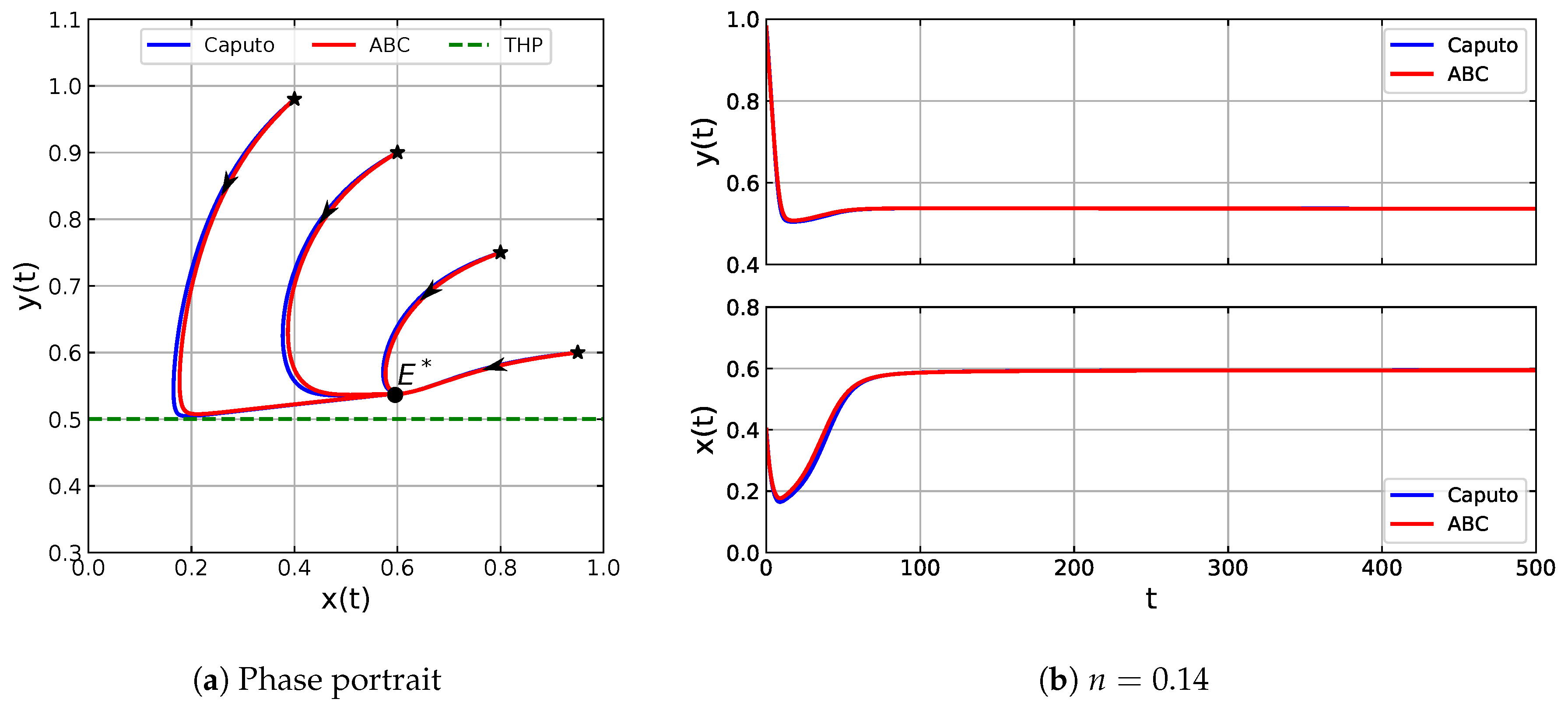
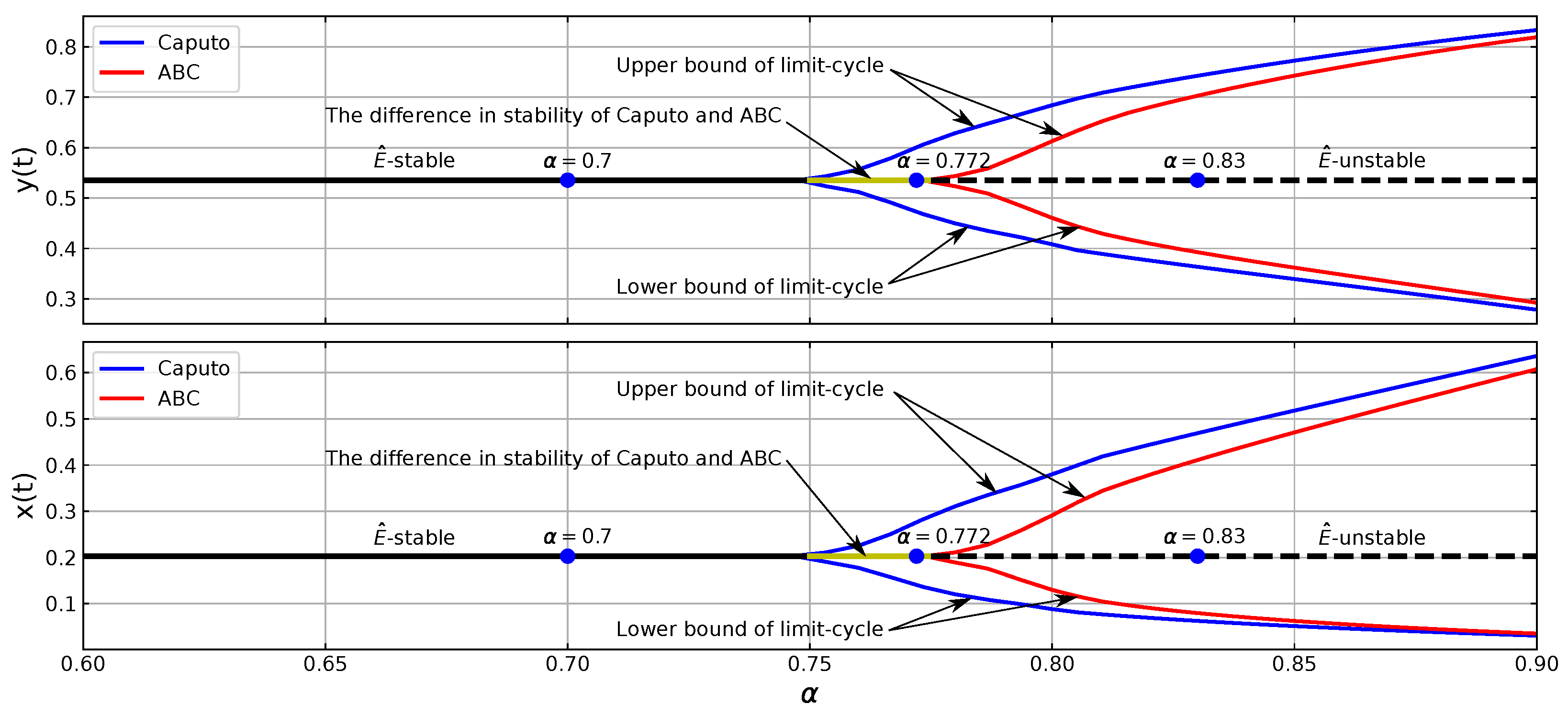
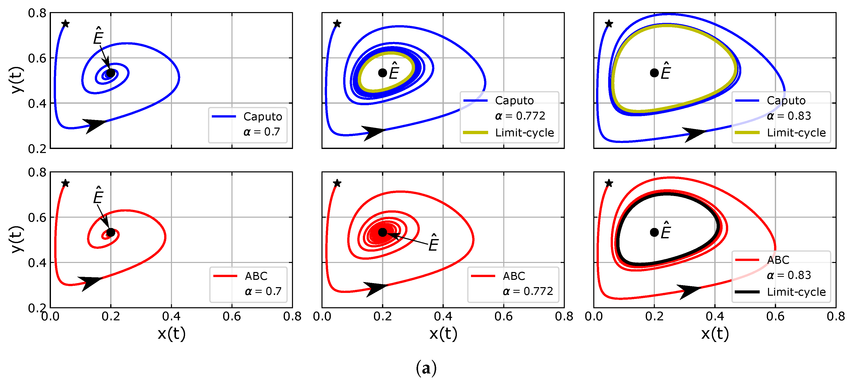
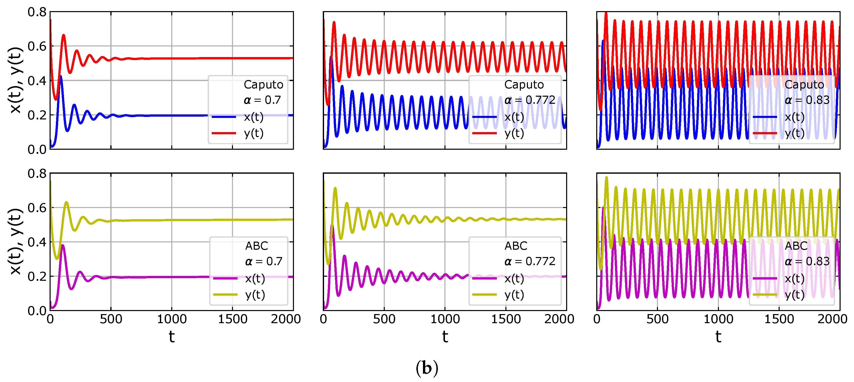
4. Numerical Simulations

In this section, the numerical simulations of Caputo model (6) and ABC model (16) are performed to illustrate the previous theoretical results. In the literature, there exist many numerical methods to solve a system of fractional differential equations, such as the Monte Carlo method [64], the Grünwald–Letnikov method [65,66] and the predictor–corrector method [67,68,69]. We apply the predictor–corrector scheme proposed by Diethelm et al. [67] to solve the Caputo fractional-order model and the predictor–corrector scheme proposed by Baleanu et al. [69] to solve the Atangana–Baleanu in Caputo sense model (ABC). Due to the limitation of field data, we use hypothetical parameter values that correspond to the theoretical results. The initial parameter values are given as follows.
r = 0.5 , K = 1 , m = 0.3 , a = 0.2 , d = 0.1 , h = 0.1 , T = 0.9 , c = 0.1 , and   α = 0.9 .
In Figure 1, we plot a bifurcation diagram by varying the conversion rate of consumed prey into predator birth n in interval [ 0.08 , 0.2 ] . We notice that the parameter values (29) and the interval 0.08 n 0.2 lead to the non-existence of equilibrium point in Ω 2 . Therefore, the first numerical simulations are focused on the dynamics in Ω 1 .
For 0.08 n < n 1 * = 0.12 , Theorem 5 states that the predator extinction point E 1 = ( 1 , 0 ) is the only equilibrium point which is asymptotically stable. To see this behavior, we take n = 0.1 and plot the phase portrait and the time series as in Figure 2. It is seen that all solutions with initial values in both Ω 1 and Ω 2 are convergent to E 1 . When the initial value is in Ω 2 , then the solution is oscillating when it crosses the threshold harvesting level and eventually converges to E 1 .
When n passes through n 1 * , the equilibrium point E 1 = ( 1 , 0 ) undergoes a forward bifurcation. In this case, there appear two equilibrium points, namely the unstable E 1 and an asymptotically stable E ^ . Figure 1 shows that E ^ is asymptotically stable if 0.12 < n n 2 * = 0.1557 . In Figure 3, we show the phase portrait and time series for the case of n = 0.14 . We see that E 0 = ( 0 , 0 ) and E 1 = ( 1 , 0 ) are saddle points, while E ^ = ( 0.5 , 0.5833 ) is asymptotically stable. This circumstance corresponds to Theorems 4–6 and 9.
Furthermore, if we increase the value of n such that n > n 2 * , then the equilibrium point E ^ loses its stability, and all solutions converge to a limit-cycle. This situation confirms the occurrence of a Hopf bifurcation driven by n. For example, if we select n = 0.2 then all equilibrium points are unstable and all solutions eventually converge to limit cycle (see Figure 4).
Now, we perform simulation using the same parameter values as in Figure 4, but with a lower threshold value, namely T = 0.5 . In this case, there is no equilibrium point E ^ in Ω 1 , and E * = ( 0.5954 , 0.5364 ) occurs in Ω 2 . According to Theorem 7, E * is asymptotically stable. Such dynamics can be clearly seen in Figure 5. This simulation shows that by applying the THP when the interior equilibrium point is stable, we can choose a suitable constant of threshold so that the existence of both prey and predator are maintained.
Notice that, in Figure 2, Figure 3, Figure 4 and Figure 5, we see that both model with Caputo operator (6) and Atangana–Baleanu operator (16) have similar dynamical behavior. The noticeable difference between them is the orbit of solutions and the diameter of the limit-cycle. In Figure 4, the diameter of the limit-cycle of the model with ABC operator looks shorter than that of the Caputo operator, which may give different dynamics when a Hopf bifurcation occurs. To get more detail view, we plot a bifurcation diagram by varying the order of the fractional derivative ( α ) (see Figure 6). In this simulation, we use parameter values as in Figure 4 and vary the order- α in the interval [ 0.6 , 0.9 ] . It is clearly seen that, besides the diameter of the limit-cycle, the bifurcation points of Caputo model and ABC model are also different. The Caputo model has an earlier bifurcation point than that of the ABC model. To show this situation, we show some numerical simulations using different values of α (see Figure 7). For α = 0.7 , the equilibrium point E ^ of both model are asymptotically stable. For α = 0.772 , the equilibrium point E ^ of the Caputo model loses its stability, while that of the ABC model remains asymtotically stable. For α = 0.83 , the equilibrium point E ^ of both models are unstable.
From the biological point of view, all previous numerical simulations show that the dynamical properties of both Caputo model and ABC model are similar except when the eigenvalues of the Jacobian matrix evaluated at the interior equilibrium point E ^ are a pair of complex conjugate with positive real part. There is a biological condition such that the prey and predator densities are eventually periodic for the Caputo model, while for ABC model, the densities of both predator and prey are eventually constant.

5. Conclusions

The dynamics of a Rosenzweig–MacArthur model with continuous threshold harvesting in predator involving the Caputo fractional-order derivative and ABC fractional-order derivative are studied. We prove the existence and uniqueness of solutions of both Caputo and ABC models. Particularly, we completely investigate the dynamics of the Caputo model including the non-negativity, boundedness, local stability, global stability, and the existence of Hopf bifurcation. From the biological meanings, the extinction of both populations never occurs since the origin point ( E 0 ) is a saddle point. Some of the situations that might occur are: (1) the predator goes extinct while the prey still survives, which is indicated by the stability of E 1 ; (2) both predator and prey co-exist and converge to a constant population density, which happens if the interior point E ^ or E * are asymptotically stable; and (3) both predator and prey co-exist where both population densities change periodically, namely when a Hopf bifurcation occurs. We show numerically that our model may undergo a forward bifurcation or a Hopf bifurcation. The Hopf bifurcation in models with both Caputo operator and ABC operator can be driven by the conversion rate of consumed prey into the predator birth rate or by the order of fractional derivative. Our numerical simulations show that the Hopf bifurcation point of both models are different.

Author Contributions

All authors equally contributed to this article. All authors have read and agreed to the published version of the manuscript.

Funding

This research was funded by the Directorate of Research and Community Service, The Directorate General of Strengthening Research and Development, the Ministry of Research, Technology, and Higher Education (Brawijaya University), Indonesia, via Doctoral Dissertation Research, in accordance with the Research Contract No. 037/SP2H/LT/DRPM/2020, dated 9 March 2020.

Acknowledgments

The authors would like to thank the reviewers for all useful and helpful comments to improve the manuscript.

Conflicts of Interest

All authors report no conflict of interest relevant to this article.

References

  1. Rosenzweig, M.L.; MacArthur, R.H. Graphical representation and stability conditions of predator-prey interactions. Am. Nat. 1963, 97, 209–223. [Google Scholar] [CrossRef]
  2. Moustafa, M.; Mohd, M.H.; Ismail, A.I.; Abdullah, F.A. Stage structure and refuge effects in the dynamical analysis of a fractional order Rosenzweig-MacArthur prey-predator model. Prog. Fract. Differ. Appl. 2019, 5, 49–64. [Google Scholar] [CrossRef]
  3. Beay, L.K.; Suryanto, A.; Darti, I.; Trisilowati, T. Hopf bifurcation and stability analysis of the Rosenzweig-MacArthur predator-prey model with stage-structure in prey. Math. Biosci. Eng. 2020, 17, 4080–4097. [Google Scholar] [CrossRef] [PubMed]
  4. González-Olivares, E.; Ramos-Jiliberto, R. Dynamic consequences of prey refuges in a simple model system: More prey, fewer predators and enhanced stability. Ecol. Model. 2003, 166, 135–146. [Google Scholar] [CrossRef]
  5. Chen, L.; Chen, F.; Chen, L. Qualitative analysis of a predator–prey model with Holling type II functional response incorporating a constant prey refuge. Nonlinear Anal. Real World Appl. 2010, 11, 246–252. [Google Scholar] [CrossRef]
  6. Almanza-Vasquez, E.; Ortiz-Ortiz, R.D.; Marin-Ramirez, A.M. Bifurcations in the dynamics of Rosenzweig-Macarthur predator-prey model considering saturated refuge for the preys. Appl. Math. Sci. 2015, 9, 7475–7482. [Google Scholar] [CrossRef]
  7. Das, M.; Maiti, A.; Samanta, G.P. Stability analysis of a prey-predator fractional order model incorporating prey refuge. Ecol. Genet. Genom. 2018, 7-8, 33–46. [Google Scholar] [CrossRef]
  8. Moustafa, M.; Mohd, M.H.; Ismail, A.I.; Abdullah, F.A. Dynamical analysis of a fractional-order Rosenzweig–MacArthur model incorporating a prey refuge. Chaos Solitons Fractals 2018, 109, 1–13. [Google Scholar] [CrossRef]
  9. Sarkar, K.; Khajanchi, S. Impact of fear effect on the growth of prey in a predator-prey interaction model. Ecol. Complex. 2020, 42, 100826. [Google Scholar] [CrossRef]
  10. Zu, J.; Mimura, M. The impact of Allee effect on a predator-prey system with Holling type II functional response. Appl. Math. Comput. 2010, 217, 3542–3556. [Google Scholar] [CrossRef]
  11. Pal, P.J.; Saha, T. Qualitative analysis of a predator-prey system with double Allee effect in prey. Chaos Solitons Fractals 2015, 73, 36–63. [Google Scholar] [CrossRef]
  12. Bodine, E.N.; Yust, A.E. Predator–prey dynamics with intraspecific competition and an Allee effect in the predator population. Lett. Biomath. 2017, 4, 23–38. [Google Scholar] [CrossRef]
  13. Mukherjee, D. Role of fear in predator–prey system with intraspecific competition. Math. Comput. Simul. 2020, 177, 263–275. [Google Scholar] [CrossRef]
  14. Van Den Bosch, F. Cannibalism in an age-structured predator-prey system. Bull. Math. Biol. 1997, 59, 551–567. [Google Scholar] [CrossRef]
  15. Mondal, S.; Lahiri, A.; Bairagi, N. Analysis of a fractional order eco-epidemiological model with prey infection and type 2 functional response. Math. Methods Appl. Sci. 2017, 40, 6776–6789. [Google Scholar] [CrossRef]
  16. Suryanto, A.; Darti, I.; Anam, S. Stability analysis of pest-predator interaction model with infectious disease in prey. AIP Conf. Proc. 2018, 1937, 020018. [Google Scholar] [CrossRef]
  17. Panigoro, H.S.; Suryanto, A.; Kusumawinahyu, W.M.; Darti, I. Dynamics of a fractional-order predator-prey model with infectious diseases in prey. Commun. Biomath. Sci. 2019, 2, 105–117. [Google Scholar] [CrossRef] [Green Version]
  18. Kumar, T.; And, K.; Chakraborty, K. Effort dynamics in a prey-predator model with harvesting. Int. J. Inf. Syst. Sci. 2000, 6, 318–332. [Google Scholar]
  19. Javidi, M.; Nyamoradi, N. Dynamic analysis of a fractional order prey-predator interaction with harvesting. Appl. Math. Model. 2013, 37, 8946–8956. [Google Scholar] [CrossRef]
  20. Zhu, C.; Kong, L. Bifurcations analysis of Leslie-Gower predator-prey models with nonlinear predator-harvesting. Discret. Contin. Dyn. Syst. 2017, 10, 1187–1206. [Google Scholar] [CrossRef] [Green Version]
  21. Suryanto, A.; Darti, I. Dynamics of Leslie-Gower pest-predator model with disease in pest including pest-harvesting and optimal implementation of pesticide. Int. J. Math. Math. Sci. 2019, 2019, 1–9. [Google Scholar] [CrossRef]
  22. Ang, T.K.; Safuan, H.M. Harvesting in a toxicated intraguild predator–prey fishery model with variable carrying capacity. Chaos Solitons Fractals 2019, 126, 158–168. [Google Scholar] [CrossRef]
  23. Leard, B.; Rebaza, J. Analysis of predator-prey models with continuous threshold harvesting. Appl. Math. Comput. 2011, 217, 5265–5278. [Google Scholar] [CrossRef]
  24. Bohn, J.; Rebaza, J.; Speer, K. Continuous threshold prey harvesting in predator-prey models. Int. J. Math. Comput. Sci. 2011, 5, 964–971. [Google Scholar]
  25. Rebaza, J. Dynamics of prey threshold harvesting and refuge. J. Comput. Appl. Math. 2012, 236, 1743–1752. [Google Scholar] [CrossRef] [Green Version]
  26. Lv, Y.; Yuan, R.; Pei, Y. Dynamics in two nonsmooth predator–prey models with threshold harvesting. Nonlinear Dyn. 2013, 74, 107–132. [Google Scholar] [CrossRef]
  27. Wu, D.; Zhao, H.; Yuan, Y. Complex dynamics of a diffusive predator–prey model with strong Allee effect and threshold harvesting. J. Math. Anal. Appl. 2019, 469, 982–1014. [Google Scholar] [CrossRef]
  28. Toaha, S. The effect of harvesting with threshold on the dynamics of prey predator model. J. Phys. Conf. Ser. 2019, 1341. [Google Scholar] [CrossRef] [Green Version]
  29. Panigoro, H.S.; Suryanto, A.; Kusumawinahyu, W.M.; Darti, I. Continuous threshold harvesting in a gause-type predator-prey model with fractional-order. AIP Conf. Proc. 2020, 2264, 040001. [Google Scholar] [CrossRef]
  30. Shepard, B.M.; Carner, G.R.; Barrion, A.T.; Ooi, P.A.C.; Van den Berg, H. Insects and Their Natural Enemies Associated with Vegetables and Soybean in Southeast Asia; Clemson Univ. Coastal Research: Orangeburg, SC, USA, 1999. [Google Scholar]
  31. Li, H.L.; Zhang, L.; Hu, C.; Jiang, Y.L.; Teng, Z. Dynamical analysis of a fractional-order predator-prey model incorporating a prey refuge. J. Appl. Math. Comput. 2017, 54, 435–449. [Google Scholar] [CrossRef]
  32. Das, S.; Gupta, P.K. A mathematical model on fractional Lotka-Volterra equations. J. Theor. Biol. 2011, 277, 1–6. [Google Scholar] [CrossRef]
  33. Panja, P. Dynamics of a fractional order predator-prey model with intraguild predation. Int. J. Model. Simul. 2019, 39, 256–268. [Google Scholar] [CrossRef]
  34. Suryanto, A.; Darti, I.; Panigoro, H.S.; Kilicman, A. A fractional-order predator–prey model with ratio-dependent functional response and linear harvesting. Mathematics 2019, 7, 1100. [Google Scholar] [CrossRef] [Green Version]
  35. Alidousti, J.; Ghafari, E. Dynamic behavior of a fractional order prey-predator model with group defense. Chaos Solitons Fractals 2020, 134, 109688. [Google Scholar] [CrossRef]
  36. Ghanbari, B.; Djilali, S. Mathematical analysis of a fractional-order predator-prey model with prey social behavior and infection developed in predator population. Chaos Solitons Fractals 2020, 138, 109960. [Google Scholar] [CrossRef]
  37. Xie, Y.; Wang, Z.; Meng, B.; Huang, X. Dynamical analysis for a fractional-order prey–predator model with Holling III type functional response and discontinuous harvest. Appl. Math. Lett. 2020, 106, 106342. [Google Scholar] [CrossRef]
  38. Sekerci, Y. Climate change effects on fractional order prey-predator model. Chaos Solitons Fractals 2020, 134, 109690. [Google Scholar] [CrossRef]
  39. Caputo, M. Linear models of dissipation whose Q is almost fFrequency independent–II. Geophys. J. Int. 1967, 13, 529–539. [Google Scholar] [CrossRef]
  40. Atangana, A.; Baleanu, D. New fractional derivatives with nonlocal and non-singular kernel: Theory and application to heat transfer model. Therm. Sci. 2016, 20, 763–769. [Google Scholar] [CrossRef] [Green Version]
  41. Atangana, A.; Koca, I. Chaos in a simple nonlinear system with Atangana–Baleanu derivatives with fractional order. Chaos Solitons Fractals 2016, 89, 447–454. [Google Scholar] [CrossRef]
  42. Tajadodi, H. A Numerical approach of fractional advection-diffusion equation with Atangana–Baleanu derivative. Chaos Solitons Fractals 2020, 130, 109527. [Google Scholar] [CrossRef]
  43. Ghanbari, B.; Kumar, D. Numerical solution of predator-prey model with Beddington-DeAngelis functional response and fractional derivatives with Mittag-Leffler kernel. Chaos Interdiscip. J. Nonlinear Sci. 2019, 29, 063103. [Google Scholar] [CrossRef] [PubMed]
  44. Morales-Delgado, V.F.; Gómez-Aguilar, J.F.; Saad, K.; Escobar Jiménez, R.F. Application of the Caputo-Fabrizio and Atangana-Baleanu fractional derivatives to mathematical model of cancer chemotherapy effect. Math. Methods Appl. Sci. 2019, 42, 1167–1193. [Google Scholar] [CrossRef]
  45. Shah, S.A.A.; Khan, M.A.; Farooq, M.; Ullah, S.; Alzahrani, E.O. A fractional order model for Hepatitis B virus with treatment via Atangana–Baleanu derivative. Phys. A Stat. Mech. Its Appl. 2020, 538, 122636. [Google Scholar] [CrossRef]
  46. Bourafa, S.; Abdelouahab, M.S.; Moussaoui, A. On some extended Routh–Hurwitz conditions for fractional-order autonomous systems of order α∈(0,2) and their applications to some population dynamic models. Chaos Solitons Fractals 2020, 133. [Google Scholar] [CrossRef]
  47. Ahmed, E.; El-Sayed, A.; El-Saka, H.A. On some Routh–Hurwitz conditions for fractional order differential equations and their applications in Lorenz, Rössler, Chua and Chen systems. Phys. Lett. A 2006, 358, 1–4. [Google Scholar] [CrossRef]
  48. Petras, I. Fractional-Order Nonlinear Systems: Modeling, Analysis and Simulation; Springer: London, UK; Beijing, China, 2011. [Google Scholar]
  49. Diethelm, K. The Analysis of Fractional Differential Equations: An Application-Oriented Exposition Using Differential Operators of Caputo Type; Springer: Braunschweig, Germany, 2010. [Google Scholar]
  50. Podlubny, I. Fractional Differential Equations: An Introduction to Fractional Derivatives, Fractional Differential Equations, to Methods of Their Solution and Some of Their Applications; Academic Press: San Diego CA, USA, 1999. [Google Scholar]
  51. Vargas-De-León, C. Volterra-type Lyapunov functions for fractional-order epidemic systems. Commun. Nonlinear Sci. Numer. Simul. 2015, 24, 75–85. [Google Scholar] [CrossRef]
  52. Huo, J.; Zhao, H.; Zhu, L. The effect of vaccines on backward bifurcation in a fractional order HIV model. Nonlinear Anal. Real World Appl. 2015, 26, 289–305. [Google Scholar] [CrossRef]
  53. Abdelouahab, M.S.; Hamri, N.E.; Wang, J. Hopf bifurcation and caos in fractional-order modified hybrid optical system. Nonlinear Dyn. 2012, 69, 275–284. [Google Scholar] [CrossRef]
  54. Deshpande, A.S.; Daftardar-Gejji, V.; Sukale, Y.V. On Hopf bifurcation in fractional dynamical systems. Chaos Solitons Fractals 2017, 98, 189–198. [Google Scholar] [CrossRef]
  55. Diethelm, K. A fractional calculus based model for the simulation of an outbreak of dengue fever. Nonlinear Dyn. 2013, 71, 613–619. [Google Scholar] [CrossRef]
  56. Moustafa, M.; Mohd, M.H.; Ismail, A.I.; Abdullah, F.A. Dynamical analysis of a fractional-order eco-epidemiological model with disease in prey population. Adv. Differ. Equ. 2020, 2020, 48. [Google Scholar] [CrossRef]
  57. Li, Y.; Chen, Y.; Podlubny, I. Stability of fractional-order nonlinear dynamic systems: Lyapunov direct method and generalized Mittag–Leffler stability. Comput. Math. Appl. 2010, 59, 1810–1821. [Google Scholar] [CrossRef] [Green Version]
  58. Odibat, Z.M.; Shawagfeh, N.T. Generalized Taylor’s formula. Appl. Math. Comput. 2007, 186, 286–293. [Google Scholar] [CrossRef]
  59. Matignon, D. Stability results for fractional differential equations with applications to control processing. Comput. Eng. Syst. Appl. 1996, 2, 963–968. [Google Scholar]
  60. Kuznetsov, Y.A. Elements of Applied Bifurcation Theory, 3rd ed.; Springer: New York, NY, USA, 2004. [Google Scholar]
  61. Baisad, K.; Moonchai, S. Analysis of stability and Hopf bifurcation in a fractional Gauss-type predator–prey model with Allee effect and Holling type-III functional response. Adv. Differ. Equ. 2018, 2018. [Google Scholar] [CrossRef] [Green Version]
  62. Li, X.; Wu, R. Hopf bifurcation analysis of a new commensurate fractional-order hyperchaotic system. Nonlinear Dyn. 2014, 78, 279–288. [Google Scholar] [CrossRef]
  63. Tavazoei, M.S.; Haeri, M. A proof for non existence of periodic solutions in time invariant fractional order systems. Automatica 2009, 45, 1886–1890. [Google Scholar] [CrossRef]
  64. Fulger, D.; Scalas, E.; Germano, G. Monte Carlo simulation of uncoupled continuous-time random walks yielding a stochastic solution of the space-time fractional diffusion equation. Phys. Rev. E 2008, 77, 021122. [Google Scholar] [CrossRef] [Green Version]
  65. Scherer, R.; Kalla, S.L.; Tang, Y.; Huang, J. The Grünwald–Letnikov method for fractional differential equations. Comput. Math. Appl. 2011, 62, 902–917. [Google Scholar] [CrossRef] [Green Version]
  66. Suryanto, A.; Darti, I. Stability analysis and nonstandard Grünwald-Letnikov scheme for a fractional order predator-prey model with ratio-dependent functional response. AIP Conf. Proc. 2017, 1913, 020011. [Google Scholar] [CrossRef]
  67. Diethelm, K.; Ford, N.J.; Freed, A.D. A predictor-corrector approach for the numerical solution of fractional differential equations. Nonlinear Dyn. 2002, 29, 3–22. [Google Scholar] [CrossRef]
  68. Wang, Z. A numerical method for delayed fractional-order differential equations. J. Appl. Math. 2013, 2013, 256071. [Google Scholar] [CrossRef]
  69. Baleanu, D.; Jajarmi, A.; Hajipour, M. On the nonlinear dynamical systems within the generalized fractional derivatives with Mittag–Leffler kernel. Nonlinear Dyn. 2018, 94, 397–414. [Google Scholar] [CrossRef]
Figure 1. Bifurcation diagram of Caputo model (6) and ABC model (16) driven by the conversion rate of consumed prey into predator birth ( n ) with constant parameter values (29). There exists two bifurcations namely a forward bifurcation which occurs when n passes through n 1 * 0.12 , and a Hopf bifurcation which occurs when n passes through n 2 * 0.1557 .
Axioms 09 00122 g001
Figure 2. Numerical simulations of Caputo model (6) and ABC model (16) with parameter values (29) and n = 0.1: Figure (a) phase portrait; and Figure (b) time series.
Axioms 09 00122 g002
Figure 3. Numerical simulations of Caputo model (6) and ABC model (16) with parameter values (29) and n = 0.14: Figure (a) phase portrait; and Figure (b) time series.
Axioms 09 00122 g003
Figure 4. Numerical simulations of Caputo model (6) and ABC model (16) with parameter values (29) and n = 0.2: Figure (a) phase portrait; and Figure (b) time series.
Axioms 09 00122 g004
Figure 5. Numerical simulations of Caputo model (6) and ABC model (16) with parameter values (29), n = 0.2 and T = 0.5.
Axioms 09 00122 g005
Figure 6. Bifurcation diagram of Caputo model (6) and ABC model (16) driven by the order of the fractional-derivative ( α ) with constant parameter values (29) and n = 0.2 . There exists a Hopf bifurcation where the bifurcation points of the Caputo model and ABC model are different.
Axioms 09 00122 g006
Figure 7. Numerical simulations of Caputo model (6) and ABC model (16) with parameter values (29), n = 0.2 , and α = { 0.7 , 0.772 , 0.83 } : Figure (a) phase portrait; and Figure (b) time series.
Axioms 09 00122 g007aAxioms 09 00122 g007b
Table 1. Description of variables and parameters of the model (1).
Variables and ParametersDescription
x ( t ) The density of prey
y ( t ) The density of predator
rThe intrinsic growth rate of prey
KThe environmental carrying capacity of prey
mThe maximum uptake rate for prey
nThe conversion rate of consumed prey into predator birth
aThe environment protection for prey
dThe natural death rate of predator
hThe harvesting rate
cThe half saturation constant for harvesting
TThe threshold level of harvesting
Publisher’s Note: MDPI stays neutral with regard to jurisdictional claims in published maps and institutional affiliations.

