Nonlinear Approximations to Critical and Relaxation Processes

Materialica+ Research Group, Bathurst St. 3000, Apt. 606, Toronto, ON M6B 3B4, Canada
Axioms 2020, 9(4), 126; https://0-doi-org.brum.beds.ac.uk/10.3390/axioms9040126
Submission received: 5 September 2020
/
Revised: 21 October 2020
/
Accepted: 22 October 2020
/
Published: 28 October 2020
(This article belongs to the Special Issue Nonlinear Analysis and Optimization with Applications)
Abstract
:We develop nonlinear approximations to critical and relaxation phenomena, complemented by the optimization procedures. In the first part, we discuss general methods for calculation of critical indices and amplitudes from the perturbative expansions. Several important examples of the Stokes flow through 2D channels are brought up. Power series for the permeability derived for small values of amplitude are employed for calculation of various critical exponents in the regime of large amplitudes. Special nonlinear approximations valid for arbitrary values of the wave amplitude are derived from the expansions. In the second part, the technique developed for critical phenomena is applied to relaxation phenomena. The concept of time-translation invariance is discussed, and its spontaneous violation and restoration considered. Emerging probabilistic patterns correspond to a local breakdown of time-translation invariance. Their evolution leads to the time-translation invariance complete (or partial) restoration. We estimate the typical time extent, amplitude and direction for such a restorative process. The new technique is based on explicit introduction of origin in time as an optimization parameter. After some transformations, we arrive at the exponential and generalized exponential-type solutions (Gompertz approximants), with explicit finite time scale, which is only implicit in the initial parameterization with polynomial approximation. The concept of crash as a fast relaxation phenomenon, consisting of time-translation invariance breaking and restoration, is advanced. Several COVID-related crashes in the time series for Shanghai Composite and Dow Jones Industrial are discussed as an illustration.
1. Introduction
Let the function of a real variable be defined by some rather complicated problem. The variable can represent, e.g., a coupling constant or concentration of particles. Of course, one should strive to find an exact solution to the problem [1,2]. Among such exact solutions one can find the solution to the celebrated Kondo problem and its thermodynamics. In a number of cases important for optical applications, such as Bessel beams and its generalizations [3], one can find an intriguing physics already within the linear wave equation. In optics, there are a variety of exact solutions: spatial, temporal, dark optical solitons and breathers all follow from the celebrated nonlinear Schrödinger equation and its modifications [4]. The so-called spatiotemporal X-waves, another type of the closed-form solutions are being studied as well (see, e.g., [5]).
What if such a problem does not allow for an explicit solution for the sought function? Let us assume that some kind of perturbation theory is still possible to develop, so that it generates formal power series about the point , , for the function in question [6]. The perturbation methods can generate the series (often slowly) convergent for all x smaller than the radius of convergence, or the series divergent for all x, except .
Our task is to recast the series (2) into some convergent expressions by means of a nonlinear analytical constructs, the so-called approximants. When literally all of the terms in divergent series are known, one can invoke Euler of Borel summation [8]. Even for convergent series there is still a problem of how to continue the expansion outside of radius of convergence [9], where the approximants could be useful.
However, in realistic problems, only a few terms on the RHS of (1) can be calculated, and applying various approximants is the only available analytical option for the truncated series (5) and (A6). The approximants are conditioned to be asymptotically equivalent to the series (1), truncated at some finite number k. However, the approximants are able to generate an additional infinite number of coefficients, approximating unknown exact coefficients. Determination of the best approximant is grounded solely on the empirical, numerical convergence [9], of the sequences of approximants.
One can always attempt to extrapolate the perturbative results by means of the Padé approximants [6,9]. The Padé approximants can be understood as the ratio of two polynomials and of the order M and N, respectively. The diagonal Padé approximant of order N corresponds to the case of . Conventionally, . The coefficients of the polynomials are derived directly from the asymptotic equivalence with the given power series for the sought function . Sometimes, when there is a need to stress the role of , we write .
The Padé approximant might possess a pole associated with a finite critical point, but can only produce an integer critical index. While usually critical indices are not integers. The same concerns the large-variable behavior where the power of x produced from extrapolation with some form of Padé approximants is always an integer. Unfortunately, solutions to many problems exhibit irrational functional behavior. Such a behavior cannot be properly described by the standard rational Padé approximants. However, it would be highly desirable to modify somehow the familiar technique of Padé approximants in order to take into account the irrational behavior. Such modification can be performed by separating the sought modification of the Padé approximants into two factors [10]. The first factor is to be expressed as an iterated root or factor approximant [11,12]. It is specifically designed to take care of the irrational part of the solution. The second factor is simply a diagonal Padé approximant, and it is supposed to take care of the rational part of the solution. We arrive thus to the corrected Padé approximants. They appear to be applicable to a larger class of problems, even when the standard Padé technique is not applicable [11].
Many examples of application of the Padé approximants as well as their theoretical modifications, can be found in [13], including some important applications to aerodynamics and boundary layer problems [14]. The so-called two-point Padé is applied for interpolation, when in addition to the expansion about , given by (1), additional information is available and contained in the asymptotic power series expansion about , [8]. The two-point Padé approximant has the same form as the standard Padé approximant, but with the coefficients expressed through and .
The idea of combining information coming from the different limits appear to be fruitful and can be exploited for different types of approximants and various forms of asymptotic expansions [11,12,15,16]. Various self-similar approximants also allow extrapolating and interpolating between the small-variable and large-variable asymptotic expansions, as discussed recently in [16]. The key to the success is to introduce the so-called control functions to allow “to sew” the two limit-cases together in the form most natural for each concrete problem [11,12,15,16,17]. The example of such an approach is brought up in Appendix B. Although the expansions for small and large couplings are very bad, the resulting approximants are in a good agreement with the numerical data.
There are four main technical approaches to the approximants constructions, all aimed to optimize their performance. The first approach is conventional, also called accuracy-through order. It is based on progressive improvement of quality of approximants with adding new information through the higher-order coefficients, with the approximants becoming more and more complex. It is exemplified in construction of Pad’e and Euler super-exponential approximants [8], factor, root and additive approximants [11,12,16]. The latter “cluster” of approximations was derived based on the ideas of self-similar approximation theory, a close relative of the field-theoretic renormalization group [17]. The property of self-similarity is discussed in Section 3.1.
The second approach leads to corrected approximants. The idea is to ensure the correct form of the solution already in the starting approximation with some initial parameters. The initial parameters should be corrected by asymptotically matching with the truncated series/polynomial regressions in increasing orders. Thus, instead of increasing the order of approximation, one can correct the parameters of the initial approximation [11,12]. The form of the solution is not getting more complex, but the parameters take more and more complex form with increasing order.
In the third approach, predominantly adopted in Section 3, we keep the form and order of approximants the same in all orders, but let the series/regressions evolve into higher orders. Independent on the order of regression, we construct the same approximant, based on the first-order terms solely, only with the parameters changing with increasing order of regression. In the framework of such effective first-order theories, we employ exponential approximants and their extensions.
In the fourth approach, the critical index is treated as a vital part of optimization procedure. The critical index plays the role of a control parameter, to be determined from the optimization procedure described in Section 2.2, following Gluzman and Yukalov [18]. Different optimization techniques based on introduction of control parameters were proposed in [19,20].
The problems arising in approximation theory can vary. Note that, for a recovery problem, when measurements of the sought function are given for some finite set of points, there is Prony’s method available, with the sought function represented as sums of polynomial or exponential functions combined with periodic functions [21]. For approximation of a continuous function on the interval , one can use Bernstein polynomials [22]. However, the two methods do not allow for inclusion of the asymptotic information.
Prony’s and Bernstein methods are numerical and work only for interpolation problems. The latter method was further adapted to the region , and applied in [23]. The technique of Cioslowski [23] allows for incorporation of the asymptotic information. The technique of self-similar roots [24] allows us to solve the same problems as in [23], but without resorting to fitting [23,24].
Our methods are analytical, user-friendly and applicable to the most difficult extrapolation problem [11,12,16], involving explicit calculation of various critical indices and amplitudes, with novel applications to finding relaxation times. However, our methods remain applicable also for various interpolation problems [11,12,16,24] (see also Appendix B).
It is likely impossible to find the same approximant to be the best for each and every realistic problem. Based on the same asymptotic information, such as series coefficients, thresholds, critical indices, and correction to scaling indices, one can construct not only Padé but quite a few different approximants, such as corrected Padé, additive, -additive, etc. [12,16]. It is feasible that for each problem one can find an optimal different approximant. We think that the idea behind the method of corrected approximants [11,12,16], is the most progressive, since it allows to combine the strength of a few methods together and proceed, in the space of approximations, with piece-wise construction of the approximation sequences, as pointed out recently by Gluzman [16].In the following sections, we present a more expended description of the concept of approximants, applied now both to critical and relaxation phenomena, extending the earlier work of Chapter 1 of the book [12].
2. Critical Index and Relaxation Time
The function of a real variable x exhibits critical behavior, with a critical index , at a finite critical point , when
The definition covers the case of negative index when function can tend to infinity, or the sought function can tend to zero if the index is positive. Sometimes, the values of critical index and critical point are known from some sources, and the problem consists in finding the critical amplitude A, as extensively exemplified in [11].
The case when critical behavior occur at infinity,
can be analyzed similarly. It can be understood as the particular case with the critical point positioned at infinity.
Critical phenomena are ubiquitous [18], ranging from the field theory to hydrodynamics. It is vital to explain related critical indices theoretically. Regrettably, for realistic physical systems, one can as a rule learn only its behavior at small variable,
which follows form some perturbation theory. The function is approximated by an expansion
Most often one finds that such expansions give numerically divergent results, valid only for very small or very large x (see Appendix B). Constructively, the expansion is treated as a polynomial of the order k. Sometimes, theoretically, one even has a convergent series, resulting in a rather good numerically convergent, truncated polynomial approximations (A6). However, there is still a problem of extrapolating outside of the region of numerical convergence, where the critical behavior sets in. Three examples of such type are given in Appendix A, based on the results of Chapter 7 of the book [12].
The discussion below traces the basic ideas from Chapter 1 of the book [12]. One can always express the critical index directly by using its definition, and find it as the limit of explicitly expressed approximants. For instance, critical index can be estimated from a standard representation as the following derivative
as , thus defining the critical index as the residue in the corresponding single pole. The pole corresponds to the critical point . The critical index corresponds to the residue
To the -transformed series one is bound to apply the Padé approximants [6]. Moreover, the whole table of Padé approximants can be constructed [9], That is, the Padé method does not lead to a unique algorithm for finding critical indices. procedure. Basically, different values are produced by different Padé approximants. Then, it is not clear which of these estimates to prefer. The standard approach consists in applying a diagonal Padé approximants [6].
When a function, at asymptotically large variable, behaves as in (3), then the critical exponent can be defined similarly, by means of the transformation. It is represented by the limit
Assume that the small-variable expansion for the function is given. In order for the critical index to be finite, it is necessary to take only the approximants behaving as as . It leaves us no choice but to select the non-diagonal approximants, so that the corresponding approximation is finite. One can also apply, in place of Padé, some different approximants [12,16]. The examples of application of the Padeé methods are given in Appendix A, based on the results first obtained in Chapter 1 of the book [12].
To simplify and standardize calculations different, and more powerful, approximants, called self-similar factor approximants, are introduced in [25]. The singular solutions emerging from factor approximants correspond to critical points and phase transitions [25], including also the case of singularity located at ∞. When the series is long, one would expect that the accuracy is going to improve with increasing numbers of terms. Sometimes, an optimum is achieved for some finite number of terms, reflecting the asymptotic nature of the underlying series. It is very difficult to improve the quality of results produced by the factor approximants, when the series are short. Some suggestions on such improvement were advanced by Gluzman [12].
In some simple but rather important cases of ODEs, the factor approximants allow to restore exact solutions, such a bell soliton, kink soliton, logistic equation solution and instanton-type solution [26]. However, as pointed out in the Introduction, such cases are quite special, and only an approximate solution could be found in many important cases [26,27]. More information about various methods of calculating critical index, amplitude and critical point can be found in [11,12,16].
2.1. Relaxation Time
Consider the case of relaxation behavior when a function at asymptotically large variable decays as
with negative . Formally, the relaxation time is . It can be found as the limit
As in the case of critical behavior considered above, the small-variable expansion for the function is given by the sum . The effective relaxation time can be expressed in terms of the small-variable expansion as follows,
It can be expanded in powers of t, leading to
The coefficients are easily expressed through of the original series (1). Let us apply to the obtained expansion the self-similar or Padé approximants, That is, we have to derive an approximant whose limit
gives the relaxation time
In such approach, the amplitude A does not enter the consideration. In practice, one can indeed construct the approximants with such required behavior. The complete approximant for the sought function denoted below as , can be constructed as well. Even some ad hoc forms satisfying some general symmetry requirements can be suggested, as in Section 3.
As an illustration, let us find in explicit form under some simple assumptions concerning its asymptotic behaviors. Assume simply that there are two distinct exponential behaviors for short and long times with two different , and the transition from short to long time behavior also occurs at the duration of some third characteristic time . The characteristic times can be found from the short-time expansion. The simple approximation to the effective relaxation time, expressed in second order of (12), can be written down in the spirit of Yukalov and Gluzman [28] as follows:
so that for negative we have
In the theory of reliability, the failure (hazard) rate or mortality force [29] is analogous to the inverse effective relaxation time, and the model of the type of formula (13) is known as the Gompertz–Makeham law of mortality.
The complete approximant corresponding to (13) is reconstructed after elementary integration
with all unknown constituents of (13) expressed explicitly, from the asymptotic equivalence with the power-series,
Most interesting, as the linear decay (growth) term in the formula for disappears, we arrive in different notations to the Gompertz function (54),
employed in calculations of Gluzman [30]. In this case, we have the effective relaxation time decaying (growing) exponentially with time. In Section 3, we apply this method of finding the effective relaxation time for time series.
2.2. Critical Index as Control Parameter. Optimization Technique
The function’s critical behavior follows from extrapolating the asymptotic expansion (1) to finite or large values of the variable. Such an extrapolation can be accomplished by means of a direct technique just discussed above. However, its successful application requires knowledge of a large number of terms in the expansion. However, it is also possible to obtain rather good estimates for the critical indices from a small number of terms in the asymptotic expansion [12,18]. To this end, we can employ the self-similar root approximants given by (17). The external power is to be determined here from additional conditions. More detailed explanations and more examples can be found in the book [12].
The self-similar root approximant has the following general form [15],
In principle, all the parameters may be found from asymptotic equivalence with a given power series.
The large-variable power in Equation (3) could be compared with the large-variable behavior of the root approximant (17),
where
This comparison yields the relation defining the external power when is known. This way of defining the external power is used when the root approximants are applied for interpolation. The root approximants (17) are applied in Appendix B, in the context of interpolation problem, for construction of accurate formulas valid for all values of x.
Consider an exceptionally difficult situation of an extrapolation problem: the large-variable behavior of the function is not known and is not given. In addition, the critical behavior can happen at a finite value of the variable x. The method for calculating the critical index by employing the self-similar root approximants was developed by Gluzman and Yukalov [18].
In such approach, we construct several root approximants , and the external power plays the role of a control function. The sequence of approximants is considered as a trajectory of a dynamical system. The approximation order k plays the role of discrete time. A discrete-time dynamical system or the approximation cascade consists of the sequence of approximants. The cascade velocity is defined by Euler discretization formula [31,32,33]
The effective limit of the sequence of approximants corresponds to the fixed point of the cascade. Based on just a few approximants, the cascade velocity has to decrease. In such a sense, the sequence appears to be convergent. The control functions , have to minimize the absolute value of the cascade velocity
A finite critical point , in the kth approximation, is to be obtained from Equation (17) by imposing the condition on the critical behavior expressed by (2),
Its finite solution is denoted as .
The critical index in the kth approximation is given by the limit
In the case of the critical behavior at infinity, when , the critical index is
Thus, to find the critical indices, the control functions have to be found. The minimization of the cascade velocity (50) is complicated. Equation (21) contains two control functions, and . Nevertheless, the problem can be resolved.
This can be done in two ways. The first constructive approach notices that should be close to . Then, we arrive to to the minimal difference condition
One should typically find a solution of the simpler equation
The control functions , characterizing the critical behavior of , become the numbers . We simply write .
In the vicinity of a finite critical point, the function behaves as
The condition (25) is expressed as follows,
For the critical behavior at infinity, it is expedient to introduce the control function
The large-variable behavior reads as
As a result, the minimal difference condition is reduced to the equation
The alternative equation for the control functions also follows from the minimal velocity condition (21), and is called the minimal derivative condition
In practice, we have to solve the equation
To apply this condition, we have first to extract from the function its non-divergent parts. If the critical point is finite, one can study the residue of the function , expressed as
Thus, from Equation (32), we arrive to the condition
When the critical behavior occurs at infinity, then we can consider the limiting form of the amplitude and reduce Equation (32) to the form
The final estimate for the critical index is given by a simple average of the minimal difference and minimal derivative results.
The technique reviewed in Section 2.2, following Chapter 1 of the book [12], turned out to be useful in calculating the critical properties of the classical analog of the graphene-type composites with varying concentration of vacancies [34].
2.3. Examples: Permeability in the Two-Dimensional Channels
In the cases considered below, we deal with a unique theoretical opportunity to attack the problem of critical exponent and criticality in general, directly from the solution of the hydrodynamic Stokes problem. Let us consider as example the case of the two-dimensional channel bounded by the surfaces as explained in Appendix A. Here, is termed waviness.
The permeability behaves critically [12], That is, it tends to zero as
with The permeability as a function of the waviness can be derived in the form of an expansion in powers of [35]. In the particular case of , the permeability can be found explicitly as
By setting and changing the variable one can move the critical point to infinity.
The critical index is calculated as explained above and in [18]. From the minimal-difference condition we find , with an error . From the minimal derivative condition, we obtain , with an error . The final answer is given by the average of two solutions
In another particular case considered in Chapter 1 of the book [12], for , the permeability expands as follows,
Setting and using the same technique as above the approximations for critical index are found, so that , and . Finally,
Let us also consider some examples of the numerical convergence of root approximants in high-orders, first presented in Chapter 1 of the book [12]. The technique is applied for calculating critical index . It seems instructive to consider the same two cases of permeability , but with higher-order terms, up to 16th order inclusively.
The numerical form of the corresponding expansions can be found in Appendix A (see expansions (A8) and (A14)). Concretely, we construct the iterated root approximants
The parameters have to be found from the asymptotic equivalence with the expansions. The permeability has the required critical asymptotic forms
The amplitudes are found explicitly as
To define the critical index , we analyze the differences
From the sequences , we find the related sequences of approximate values for the critical indices.
Although it is possible to investigate different sequences of the conditions , the most natural from is presented by the sequences of and , with .
The results for are shown in Table 1. We observe good numerical convergence of the approximations , to the value .
Similar results, presented in Table 2 (for ), again demonstrate rather good numerical convergence of the approximate critical indices to the value .
Comparison of the results for different parameters b allows us to think that the critical index does not depend on parameter b. In both examples considered above, the convergence sets in rather quickly.
The Padé method appears to bring convergent sequences and consistent expressions for permeability as well. Further details can be found in Appendix A. The results obtained from the two different methods well agree with each other. A similar comparison was made by Gluzman and co-authors [34] for the effective conductivity of graphene-type composites.
Consider a different case of permeability (see Appendix A and Appendix A.3). The results were first obtained in Chapter 1 of the book [12]. For the parallel sinusoidal two-dimensional channel when the walls would not touch, the permeability remains finite. It is expected to decay as a power-law as the waviness becomes large,
with negative index .
In the expansion of in small parameter , we retain the same number of terms as in the previous two examples. The numerical values of the corresponding coefficients can be found in Appendix A (see expression (A16)). The results of calculations are presented in Table 3 (for ). They show rather good numerical convergence, especially in the last column, to the value . The sequence, based on the Padé method, is convergent as well (see Appendix A and Appendix A.3).
More information on the problems of critical permeability, can be found in Appendix A. The three problems considered above are studied by applying the Padé method of Section 2 to calculate the critical index for permeability. The computations complement and confirm the results for critical index, obtained above from the optimization technique. The optimization technique works better for short truncated series, converging more quickly, while the Padé method is easier to apply for very long series. In addition, the Padé method, as well as the Padé method, when its application is appropriate, allows us to compute the critical amplitudes.
3. Relaxation Phenomena in Time Series
For the phenomenon to occur, the basic underlying symmetry must be broken. While studying the phenomenon it is important to distinguish between an explicit symmetry breaking when governing equations are not invariant under the desired symmetry and spontaneous symmetry breaking, without presence of any asymmetric cause [36]. When successful, the approach based on broken global symmetries leads to understanding of the key phenomena of magnetism, superconductivity and superfluidity. On the other hand, when some global inherent symmetry can be recognized in physical quantities, we arrive to the gloriously successful theory of critical phenomena and vital extensions of perturbation results in quantum field theories, jointly called renormalization group (RG) [17,37]. In a nutshell, we suggest below how to apply symmetry considerations and RG-inspired methods to the sharp moves which occur in time series, with the most notable examples given by stock market crashes.
Assume that numerical data on the time series variable (e.g., price) s is given for some time t segment. Typically, one considers values for given at equidistant successive moments in time , with [38].
In the study of time series, one is interested in the extrapolated to future value of s. In financial mathematics, one is particularly interested in the predicted value of log return [38,39],
One can see from the definition that we are really interested in the quantity , to be called return. Let us place the origin at the very beginning of the time interval, setting also . Naturally, one is interested in the value of , allowing to find at a later time. Since the approach developed in [30,38] is invariant with regard to the time unit choice, we consider temporal points of the dataset as integer, while considering the actual time variable as continuous.
Modern physics when applied to financial theory is concerned with ergodicity violations [40,41,42,43]. Ergodicity violations may be understood as a manifestation of a non-stationarity, or violation of time-invariance of random process. Metastable phases in condensed matter also defy ergodicity over long observation timescales. In special quantum systems of ultracold atoms, spontaneous breaking of time-translation symmetry causes the formation of temporal crystalline structures [44]. The concept of a spontaneously broken time-translation invariance can be useful for time series in application to market dynamics, as first suggested in [38]. According to Andersen, Gluzman and Sornette [38], the window of forecasting of time series describing market evolution emerges due to a spontaneous breaking/restoration of the continuous time-translation invariance, dictated by relative probabilities of the evolution patterns [45]. In turn, the probabilities are derived from the stability considerations.
The notion of probability introduced in [45] is not based on the same conventional statistical ensemble probability for a collection of people, but it is closer to the time probability, concerned with a single person living through time (see Gell-Mann and Peters [42] and Taleb [43]). Probabilistic trading patterns correspond to local breakdown of time-translation invariance. Their evolution leads to the time-translation symmetry complete (or partial) restoration. We need to estimate typical time, amplitude and direction for such a restorative process. Thus, we are not confined to a binary outcome as in [38] but attempt to estimate also the magnitude of the event.
According to Hayek [46], markets are mechanisms for collecting vast amounts of information held by individuals and synthesizing it into a useful data point [46,47], e.g., price of the stock market index dependent on time. Conversely, consolidation of knowledge is done via prices and arbitrageurs (Taleb on Hayek).
A catastrophic downward acceleration regime in the time series is known as crash [48]. Time series representing market price dynamics in the vicinity of crisis (crash, melt-up), could be treated as a self-similar evolution, because of the prevalence of the collective coherent behavior of many trading, interacting agents [45,49], including humans and machine algorithms. The dominant collective slow mode corresponding to such behavior, develops according to some law, formalized as a time-invariant, self-similar evolution. Away from crisis, there is a superposition of collective coherent mode (generalized trend) and of a stochastic incoherent behavior of the agents [39,45]. We do not attempt here to write down a generic evolution equation of behind the time series pertaining to market dynamics. Instead. we consider, locally in time, some trial functions—approximants—in the form inspired by the solutions to some well-known evolution equations. The approximants are designed to respect or violate self-similarity. If in physics the relation of phenomenon and symmetry violation is understood, in econophysics such connection is far from being clear. However, to realize the promise of econophysics [50], on a consistent basis and at par with physics achievements, one has to identify and study the phenomenon from the relevant symmetry viewpoint. Our primary goal here is not forecasting/timing the crash, but studying the crash as a particular phenomenon created by spontaneous, time-translation symmetry breaking/restoration.
Since the market dynamics is believed to be formed by a crowd (herd) behavior of many interacting agents, there are ongoing attempts to create empirical, binary-type prediction markets functioning on such principle, or mini Wall Streets [47]. Prediction markets often work pretty well, however there are many cases when they give wrong prediction or do not make any predictions at all. Such special set-ups are already very useful in reaching understanding that market crowds are correct only if they express a sufficient diversity of opinion. Otherwise, the market crowd can have a collective breakdown, i.e., is fallible, as expected by Soros [48]. In our understanding, such breakdowns amount to breaking of time-translation invariance. Restoration of the time-translation invariance—in theory—may be attributed to a small proportion of the traders having either superior information or market intellect [47]. Data from a survey conducted with high income and institutional investors show that they “generally exaggerated assessments of the risk of a stock market crash, and that these assessments are influenced by the news stories, especially front page stories, that they read” [51]. The division into two (at least) groups can be seen in the very parallel existence of future and spot markets for the same asset, such as S&P 500 index, with the futures market working 24 h. It is believed that a lot of the daily crashes, or melt-up days, start overnight. It is not that arbitrage is not effective, the spot market is just closed overnight, while the futures market operates in a discovery mode.
3.1. Self-Similarity and Time Translation Invariance
According to Isaac Newton and Murray Gell-Mann, the laws of nature are somehow self-similar. The laws of Newtonian mechanics are invariant with respect to the Galilean group, expressing Galileo’s principle of relativity [52]. The group includes time-translation invariance, or else the laws of classical mechanics are self-similar.
What should be the underlying symmetry for price dynamics? Mind that in normal times the average price trajectory is exponential, because of the compounding interests, and we enjoy an almost constant return (or price growth rate) [53]. Indeed, let be an underlying security (index) price at . Let be the fair value of the future requiring a risk associated expected return [43]. Then (see, e.g., [43]), expected forward price For example, a share of a stock would be correctly priced with the expected return calculated as the return of a risk-free money market fund minus the payout of the asset, being a continuous dividend for a stock [43]. Thus, rather simple and natural exponential estimates are constantly made for stocks and the alike. The formula for the forward price is self-similar, or time-translation invariant, as explained below.
However, as noted in [48,53], prices often significantly deviate from such a simple description. Bubbles can be formed, as well as other presumed patterns of technical analysis. Asset prices strongly deviate from the fundamental value over significant intervals of time. The fundamental value is not truly observable, making definition of such intervals somewhat elusive. There are some very real mechanisms in work, acting to increase and even accelerate the deviation from fundamental value. The causes of deviation could be “option hedging, portfolio insurance strategies, leveraging and margin requirements, imitation and herding behavior”, as is the authoritative opinion expressed in [48,53].
Recall also that meaningful technical analysis starts from recasting the time series data using some polynomial representation to serve as the expansion [38]. The regression is constructed in standard fashion by minimizing mean-square deviation, with the effective result that the high-frequency component of the price is getting average out. Then, one can consider self-similarity in averages [49]. Indeed, the standard polynomial regressions are invariant under time-translation, retaining their form after arbitrary selection of origin of time with simple redefinition of all parameters. The position of origin in time can be explicitly introduced into the regression formula and included into the coefficients, but actual results of calculations with any arbitrary chosen origin will remain the same. Such property can be expressed as some symmetry.
We put forward the idea that it is the onset of broken time-translation invariance that signifies the birth of a bubble, or of some other temporal pattern preceding a crash. End of pattern corresponds to the restoration of time-translation invariance, partially or fully. Our task is to express this idea in quantitative terms by making explicit transformation from the regression-based technical analysis to the valuation formula in the exponential form, taking into account strong deviations from the standard valuation formulae.
Assume that a time series dynamics is predominantly governed by its own internal laws. This is the same as to write down a self-similar evolution for the marker price s [54], meaning that, for arbitrary shift , one can see that
with the initial condition [55,56]. The value of the self-similar function s in the moment with given initial condition, is the same as in the moment t, with the initial condition shifted to the value of s in the moment .
When t stands for true time, the property of self-similarity means the time-translation invariance. Formally understood, Equation (43) gives a background for the field-theoretical RG, with addition of some perturbation expansion for the sought quantity, which should be resummed in accordance with self-similarity expressed in the form of ODE [55,56,57]. The time-translation invariance expressed by (43) means that the law for price evolution exists and remains unchanged with time, with proper transformation of the initial conditions [52]. The role of perturbation expansion when price dynamics is concerned, is accomplished by meaningful technical analysis, by recasting data in the form of some polynomial representation [38]. There is no formal difference in treating polynomials and expansions, as already mentioned in Section 2.
Consider first the simplest case of technical analysis. The linear function can be formally considered as the function of time and initial condition a, namely and . The linear function (regression) is self-similar, or time-translation invariant, as can be checked directly, by substitution into (43).
Through some standard procedure, let us obtain the linear regression on the data around the origin , so that
Note that the position of origin is arbitrary, and it can be moved to arbitrary position given by real number r, so that
with new and different coefficients. It turns out that the coefficients are related as follows
so that
By shifting the origin, we create an r-dependent form of the linear regression , which can be used constructively. Thus, instead of a single regression we have its r-replicas, equivalent to the original form of regression, and all replicas respect time-translation symmetry. In such a sense, one can speak about replica symmetry. Of course, we would like to avoid such redundancy in data parameterization and to find the origin(s) by imposing some optimal conditions (see Section 3.2).
The position of origin in time can be explicitly introduced into the regression formula and included into the coefficients, but actual results of calculations with any arbitrary chosen origin will remain the same. Such property can be expressed as some symmetry. However, intuitively, one would expect that the result of extrapolation with chosen predictors should be dependent on the point of origin r. Indeed, various patterns such as “heads and shoulders”, “cup-with-handle”, “hockey stick”, etc., considered by technical analysts do depend on where the point of origin is placed. In physics, the point of origin (Big Bang) plays a fundamental role. We should find a way to break the replica symmetry.
As discussed above, it is exponential shapes that are natural in pricing. Exponential function
with initial condition a and arbitrary satisfy functional self-similarity as well as the linear functions. It can be replicated as
Having dependent on r is going to violate the time-translation and replica symmetry. Instead of a global time-translation invariance, we have a set of r local “laws” near each point of origin. However, having r in Formula (44) fixed, by imposing some additional condition, or just being integrated out, should restore the global time-translation invariance completely as long as the exponential function is considered. Moreover, stability of the exponential function is measured by the exponential function with the same symmetry (see Formula (46)). Not only is exponential function time-translation invariant, but the expected return has the same property. For exponential functions, the expected (predicted) value of return per unit time exactly equals .
Another simple rational function, known as hyperbolic discounting function [58], where a is the initial condition and b is arbitrary, is time-translation invariant. Note that shifted exponential function with initial condition a and arbitrary b and c, is invariant under time-translation as well.
Another interesting symmetry is shape invariance [59], meaning
and an exponential function is shape invariant with , leaving the expected return unchanged. Keep in mind that our task is to calculate from the time series. In principle, one can think about breaking/restoration of shape invariance, as a guide for construction of the concrete scheme for calculations.
A critical phenomenon, an underlying symmetry of the formula for the observable, is scaling
where . The class of power laws, , with critical index , is scaling-invariant. The central task is to calculate c. The statistical renormalization group formulated by Wilson [37] explains well the critical index in equilibrium statistical systems. When information on the critical index is encoded in some perturbation expansion, one can use resummation ideas to extract the index, even for short expansions and for non-equilibrium systems [11,12,18]. Some of the methods are discussed in the preceding section (see also [12,16]).
Working with power-law functions will not leave the return unchanged. However, one can envisage the scheme with broken scaling invariance, as an alternative to the former schemes. The log-periodic solutions extend the simple scaling [60] and are extensively employed in the form of a sophisticated seven-parametric fit to long historical dataset [53], as well as of its extensions [61]. The fit is tuned for prediction of the crossover point to a crash, understood as catastrophic downward acceleration regime [48]. However, one cannot exclude the possibility of the solutions with different time symmetries (scaling and time-invariance, for instance) competing to win over, or to coexist, all measured in terms of their stability characteristics.
Our primary concern is the crash per se, not the regime preceding it. We start analyzing crashes with the polynomial approximation that respects time-translation symmetry, have the symmetry broken, and then restored (completely or partially), by means of some optimization. Such sequence ends with a non-trivial outcome: becomes renormalized , with r being found using the optimization procedure(s) defined below. We discuss in Section 2.1 a general technique for correcting directly, which accounts for higher order terms in regression, making it time-dependent.
In [38], the framework for technical analysis of time series was developed, based on second-degree regression and asymptotically equivalent exponential approximants, with some rudimentary, implicit breaking of the symmetry. We intend to go to higher-degree regressions and develop a consistent technique for explicit symmetry breaking with its subsequent restoration. According to textbooks, the fourth order should be considered as “high”. Taleb (see footnote on p. 53 in [43]) also considered models with five parameters as more than sufficient.
3.2. Optimization, Approximants, Multipliers
Higher-order regressions allow for replica symmetry. For instance, the quadratic regression can be replicated as follows:
with
With such transformed parameters, we find that In fact, one can still formulate self-similarity analogous to (43), but in vector form with increased number of parameters/initial conditions in place of a [57]. However, if only the linear part of quadratic regression, or trend, is taken into account, we return to the conventional functional self-similarity ≡ time-translation invariance, discussed above extensively.
Such effective linear/trend approach to higher-order regressions allows applying the same idea at all orders and observe how the exponential structures change with increasing regression order. Note that, in the course of trading, a common pattern is trend following, which appears to be a collective, self-reinforcing motion that, intuitively, lends itself to a self-similar description. Indeed, some participants are waiting for a market confirmation of the trend before acting on it, which in turn acts as a confirmation for others. Having a universal model explaining this dynamics (if not predicting it) would be quite useful.
To take into account the dependence on origin, the replica symmetry has to be broken. Breaking of the symmetry means the dependence on origin of actual extrapolations with non-polynomial predictors. As the primary predictors, we suggest the simplest exponential approximants considered as the function of origin r and time,
independent on the order of polynomial regression. The approximants (45) are constructed by requiring an asymptotic equivalence with the linear part of chosen polynomial regression. If the extrapolations are made by each of the approximants, they appear to be different for various r, meaning breaking of the replica symmetry and of the time-translation symmetry. Passage from polynomials to exponential functions leads to emergence of the continuous spectrum of relaxation (growth) times.
To compare the approximants quality, one can look at their stability. Stability of the approximants is characterized by the so-called multipliers defined as the variation derivative of the function with respect to some initial approximation function [45]. Following Yukalov and Gluzman [62], one can take the linear regression as zero approximation and find the multiplier
The simple structure of multipliers (46) allows avoiding appearance of spurious zeroes which often complicate analysis with more complex approximants/multipliers.
Because of the multiplicity of solutions, embodied in their dependence on origin, it is both natural and expedient to introduce probability for each solution. As explained in [45], one can introduce
with proper normalization, as shown below in Formula (48). Probability appears to be of a pure dynamic origin and is expressed only from the time series itself. When the approximants and multipliers of the first order are applied to the starting terms of the quadratic, third- or fourth-order regression, we are confined to effective first-order models, with velocity parameter from [38] dependent also on higher-order coefficients and origin.
To make extrapolation with approximants (45), one has still to know the origin. In other words, the time-translation symmetry has to be restored completely or partially, so that a specific predictor with specifically selected origin, or as close as possible to a time-translation invariant form, is devised. Fixing unique origin also selects unique relaxation (growth) time, during which the price is supposed to find a time-translation invariant state.
Exponential functions are chosen above because they are invariant under time translation. Any shift in origins is absorbed by the pre-exponential amplitude and does not influence the return R. A similar in spirit view that broken symmetries have to be restored in a correct theory was expressed by Duguet and Sadoudi [63].
In the approach predominantly adopted in this section, we keep the form and order of approximants the same in all orders, but let the series/regressions evolve into higher orders. Independent of the order of regression, we construct the same approximant, based only on the first-order terms, only with parameters changing with increasing order of regression. In the framework of the effective first-order theories, we employ exponential approximants.
Consider the value of origin as an optimization parameter [30]. To find it and restore the time-translation symmetry, we have to impose an additional condition directly on the exponential predictors with known last closing price,
One has to solve the latter equation to find the particular origin(s) . In this case, we consider a discrete spectrum of origins, consisting of several isolated values. To avoid double-counting when the last closing price enters both regression and optimization, one can determine the regression parameters in the segment limited from above by . Alternatively, one can consider the two ways to define regression parameters and choose the one which leads to more stable solutions. Unless otherwise stated, we consider that such comparison was performed and the most stable way was selected.
The extrapolation for the price is simply . The condition imposed by Equation (47) is natural, because then a first-order approximation to Formula (42), , is recovered (see, e.g., [39]), as one would expect intuitively.
The procedure embodied in (47), leads to a radical reduction of the set of r-predictors to just a few. Set of predictors and corresponding to each multiplier, define the probabilistic, poor man’s order book. Instead of an unknown to us true numbers of buy and sell orders, we calculate a priori probabilities for the price going up or down and corresponding levels. Target price is estimated through weighted averaging developed in [45,62], in its concrete form (48) given below.
For the sake of uniqueness, one can simply choose the most stable result among such conditioned predictors. One can also consider extrapolation with a weighted average of all such selected solutions. With solutions, their weighted average for the time is given as follows,
Within the discrete spectrum, we can find solutions with varying degrees of adherence to the original data. They can follow data rather closely or be loosely defined by the parameters of regression. The former could be called “normal” solutions, and tend to be less stable, with multipliers ∼1, but the latter are “anomalous” solutions, since they cut through the data and typically are the most stable with small multipliers. Anomalous solutions are crashes (meltdowns) and melt-ups. The typical situation with the solutions in the discrete spectrum is presented in Figure 1. The novel feature introduced through (48) is that averaging is performed over all approximants of the same order, compatible with constraints expressed by (47).
One can also integrate out the dependence on origin r, considered as a continuous variable, by applying an averaging technique of weighted fixed points suggested in [45]. The dependence on origin enters the integration limit through parameter T. Integration can be performed numerically for the simplest exponential predictors according to the formula
To optimize the integral, we have to impose an additional condition on the weighted average/integral. It is natural to force it to pass precisely through the last historical point.
and solve the latter equation to find the integration limit . The sought extrapolation value for the price s is simply We prefer to take into account the broadest possible region of integration. Under such conditions, if and when the solution to (50) exists, it is unique. The value of may enter the consideration twice: in the regression parameters and in the optimization condition (50). To avoid counting twice the last known value , one can slightly different definition
As an additional condition to find origin, one can also consider the minimal difference requirement on the lowest order predictors, as first suggested in [49]. Such approach is analogous to the technique discussed in Section 2.2. However, instead of a critical index, we calculate relaxation time. To this end, one has to construct the second order super-exponential approximant
and minimize its difference with the simplest exponential approximant in the time of interest . Namely, one has to find all roots of the equation
with respect to real variable r. Corresponding multiplier
can be found as well.
The discrete spectrum optimization seems to be the most natural and transparent. Our goal is to find the approximants and probabilistic distributions in the last available historical point of time series. Crashes are attributed to the stable solutions with large negative r, meaning that the origin of time has to be moved to the deep past to explain the crash in near future. Preliminary results of Gluzman [30] suggest that, in the overwhelming majority of cases, a crash is preceded by similar, asymmetric probability pattern(s), of the type shown in the figures below. As noted in [51], Kahneman and Tversky explained that people tend to judge current events by their similarity to memories of representative events.
There are also additional solutions with multipliers of the order of unity, coming from the region of moderate r, and it is often possible to find some rather stable upward solution for large positive r. One can think that, for such stable time series as describing population dynamics, only the region of moderate r gives relevant solutions, while for time series describing price dynamics all types of solutions may exist simultaneously.
Within our approach to constructing approximants, one can also try to exploit the second order terms in regression. Instead of exponential approximants, one should try some other, higher-order approximants, but with time-translation invariance property. Such approximants are presented below. They are considered ad hoc, because they can be written in closed form only in special, low-order situations. It is not feasible to extend them systematically into arbitrary high order. Hence, our interest in special forms with desired symmetry. Sometimes, it is even not possible to find stable solutions with a single approximant, but it is still possible with corrected approximants.
Recall that exponential function can be obtained as the solution to simple linear first-order ODE. In the search for second-order approximants with time-translation invariance, we turned to some explicit formulas, emerging in the course of solving some first-order ODE with added nonlinear term with arbitrary positive power, which generalizes ODE for simple exponential growth. It is known as Bertalanffy–Richards (BR) growth model [64,65]. Among its solutions in the case of second-order nonlinear term, there is a celebrated logistic function [64],
where is the initial condition. The logistic function is widely used to describe population growth phenomena and is also known to be the solution to the logistic equation of growth. The logistic function written in the form , dependent on the initial condition , with arbitrary , is time-translation invariant. One can also introduce the second-order logistic approximant which generalizes logistic function [30]. In addition to describing situations with saturation at infinity, the logistic approximant include also the case of so-called finite-time singularity, which makes it redundant, since such solutions were axiomatically excluded from the price dynamics [38].
Another solution to the BR model in the case when the nonlinear term has power only slightly differing from unity, is known as Gompertz function [64],
used to describe growth (relaxation, decay) phenomena. However, as we demonstrate in Section 2.1, it is possible to explain directly from the resummation technique leading to Formula (16), without resorting to BR. Relaxation (growth) time behaves exponentially with time. The Gompertz function is -time-translation invariant.
One can consider the second order Gompertz approximant. It simply generalizes the Gompertz function. Namely, one can find Gompertz approximant in the following form
with the multiplier
The Gompertz approximant, of course, is not limited to the situations with saturation at infinity, as it can also describe very fast decay (growth) at infinity.
With r to be found from some optimization procedure, the return R generated by Gompertz approximant is time-translation invariant and has a compact form
For small , it becomes particularly transparent:
with the pre-factor giving the return per unit time. The inverse return per unit time has the physical meaning of the effective time for growth (relaxation)
considered at the moment . Here, we employ the the effective relaxation (growth) time (see Section 2.1),
and replicate it. We find that the return for Gompertz approximant is solely determined by relaxation time
allowing to express the log return in a compact form
Thus, the return for Gompertz approximant appears as purely dynamic quantity, not involving any consent about equilibrium, fundamental value, etc. If relaxation time is found from the data to be very large as it should be close to equilibrium conditions [66], we have no potential for returns, i.e., near-equilibrium yields dull, everyday mundane events that are repetitive and lend themselves to statistical generalizations [48]. If relaxation time is anticipated to be very short, we have potentially huge returns. The far-from-equilibrium conditions give rise to unique, historic events [48], or to some very fast relaxation events/crashes. The latter condition makes real markets fragile [67].
Gompertz approximant can go at infinity faster or slower than exponential, and in some important examples such differences amounting to a few percent, can be detected. The function , could be called a gauge function for the price, expressing arbitrariness of choice of the price unit, as it does not enter the return. The time-translation invariance of return and gauge invariance for the price are considered very desirable in price model formulation [38], both properties are pertinent to exponential and Gompertz approximations for the price temporal dynamics.
We are interested in market prices on a daily level, and consider only significant market price drops/crashes with magnitude more than . Such magnitude is selected to be comparable to the typical yearly return of Dow Jones Industrial Average index. Typically, a 2% daily move is considered as big, but not at the times of various turmoils.
It is widely accepted in practical finance that asset price moves in response to unexpected fundamental information. The information can be identified as well as the tone, positive versus negative. It is found that news arrival is concentrated among days with large return movements, positive or negative [68]. Spontaneously emerging narratives, a simple story or easily expressed explanation of events, might be considered as largely exogenous shocks to the aggregate economy [51]. Simply put, one should analyze what people are talking about in the search for the source of economic fluctuations. Moreover, as in true epidemics governed by evolutionary biology, mutations in narratives spring up randomly, and if contagious generate unpredictable changes in the economy [51]. As noted by Harmon et al. [69], panic on the market can be due to external shocks or self-generated nervousness.
It is argued [70] that cause and effect can be cleanly disentangled only in the case of exogenous shocks, as it is only needed to select some interesting set of shocks to which price is likely to respond. Effects of positive and negative oil price shocks on the stock price need not be symmetric. In macroeconomics, it is even accepted that only positive changes in the price of oil have important effects. Periods dominated by oil price shocks are reasonably easy to identify, and they can indeed be considered as exogenous as well as, often, strong, although difficult to model. Oil price shocks are the leading alternative to monetary shocks and may very well have similar effects [70].
Our goal here is not to forecast/timing the crash, but to study the crash as a particular phenomenon created by spontaneous, time-translation symmetry breaking/restoration. In essence, we ask the following questions:
- What probabilistic pattern would an observer see the day before crash,
- What would be the market reaction (expressed through the index), if we are aware that a Swan of some color has already arrived?
In our opinion, in the presence of a Swan, understood as a shock of unspecified strength, the problem simplifies, because of a reduced set of outcomes, dominated by the most extreme, very stable downward solution. Consider that, in natural sciences, most efforts are dedicated to creating a correct experimental setup. Studying reaction to shock is the only current viable substitute for clean experimental conditions.
3.3. Examples
Consider as example a drop in the value of Shanghai Composite index related to the first COVID-19 crash, which occurred on 3 February 2020. With , as recommended in [38], the following data points are available,
The value of is to be “predicted”. From the whole set of daily data, we employ only several values of the closing price. Such coarse-grained description of the time series may be justified if one is interested in the phenomenon not dependent on the fine details, such as crash. In the examples presented below, we keep the number of data points per quartic regression parameter in the range 3–4. Lower order calculations can be found in [30]. Here, we show only the quartic regression
and based on it optimize approximants and multipliers. It can be replicated as follows:
with
With such transformed parameters, we have
Within the data shown in Figure 2, one can discern competing trends. First, let us show the data compared to the regression. There are two obvious trends, “up” and “down”, as can be seen in Figure 2.
Our analysis indeed finds highly probable solutions of both types, with the downward trend developing into fast exponential decay. Let us analyze the typical approximant and multiplier dependencies on origin, for fixed time . The inverse multiplier is shown as a function of the origin r in Figure 3 as well as the first-order approximant.
There are two uneven humps in the probabilistic inverse multiplier, suggesting that large negative and large positive r dominate, with more weight put on the negative region. Such dependence on r manifests the time-translation invariance violation, which should be lifted by finding appropriate origin. More details on the example can be found in [30]. Below, we discuss only the fourth-order calculations.
The results of extrapolation by method expressed by Equation (47) is given as
with relative percentage error of . There is also a less stable “upward” solution
in agreement with intuitive picture based on naive data analysis. There are also two additional solutions in between with multipliers close to 1. They do not affect averages much, but in real time the metastable solutions, similar to the metastable phases in condensed matter, may show up under special conditions. Metastable solutions when realized violate the principle of maximal stability over the observation timescale, complicating or even negating a unique forecast, based on weighted averages or the most stable solution.
Calculation of the discrete spectrum can be extended to different approximants. For instance, one can also construct the second-order Gompertz approximant introduced above, and solve the following equation on origins:
The most stable Gompertz approximant gives the most accurate estimate
with a very small error of . There are altogether five solutions to (56), in the discrete spectrum, as shown in Figure 1.
Thus, the Gompertz approximant of second order with log-time-translation invariance gives better results than symmetric exponential approximant . Although Taleb’s Black Swan did seem to materialize, the short-time stock market response was not different than in somewhat comparable instances of crashes brought up in [30], making it look like a Grey Swan. Indeed, it is plausible that the holiday season in China played the role here. It also helped our cause, effectively pinpointing the day for crash. One can think that all solutions, except the most extreme downward solution, were simply not considered.
Consider several most spectacular examples of crashes from the tumultuous spring and summer of 2020, caused by combination of economic causes such as oil anti-shock and COVID-19 related, enormous disruptions—a rare constellation of Two Swans of Gray coming together! There was a month long delay until DJ crashed. All three conspicuous crashes from March 2020 can be considered as an exponentially accelerated decay.
Black Monday I. Drop in DJ Industrial of was caused by the shock from coronavirus, to the value of 23,851, on 9 March 2020 (Black Monday I), as demonstrated in Figure 4. The data and the components defining spectrum of scenarios are presented.
Again, there are two asymmetric humps in the probabilistic space, and the region of large negative r dominates. The extrapolation by the most stable solution results in the following result,
of . There is also less stable by order of magnitude “upward” solution, as well as four additional solutions in between with multipliers of the order of unity. Using the same methodology, we obtain Gompertz approximant, and find that it gives rather good extrapolation
with a very small multiplier, and shows accuracy of . There is also an upward solution, by order of magnitude less stable. Averaging the two solutions improves the estimate to the error of only .
Black Thursday. Drop of , to the level of 21,200.6 on 12 March 2020 (Black Thursday), is also believed to be caused by the coronavirus-shock. In this case, we use the standard dataset with and the third-order regression to see the typical pattern shown in Figure 5.
There is again a marked asymmetry on the graphs for the components in the probabilistic space, as the region of large negative r prevails. The extrapolation by the most stable solution gives
bringing the numerical error . There is also a much less stable “upward” solution. Using the same methodology for finding the discrete spectrum, we obtain Gompertz approximant, and find that it gives rather good result
with a very small multiplier and an accuracy of . There is also an additional solution, even slightly more stable, leading to a super-fast decay almost to zero. Such scenario, obviously, is absent in calculations with pure exponential approximants.
Black Monday II. Consider also the massive crash of , to the value of 20,188.5 on 16 March 2020 (Black Monday II), caused also by oil anti-shock. Because the USA is the largest producer of oil, the big drop in oil prices (anti-shock) caused an effect typically attributed to oil shock. In this case, we again use the dataset of standard length with , to see the typical pattern shown in Figure 6. It demonstrates the data, approximant and multiplier.
There are two typical asymmetric humps in the probabilistic space, and the region of large negative r dominates. The extrapolation by the most stable solution gives the following values,
bringing the numerical error of . There is also much less stable “upward” solution,
as well two additional solutions in between, with multipliers of the order of unity. Using the same optimization methodology, we obtain Gompertz approximant, and find extrapolations
with accuracy of .
Fear of second wave of coronavirus. Bubble configuration corresponds to the price (index) going up monotonously, with rapid change of direction at some point, during the time scale of order of the time-series resolution. The growth finally becomes unsustainable. The crash of 11 June 2020 had started overnight. The index dropped to 25,128.2, corresponding to a mini-crash of 6.9%. For the the dataset of length , we observe almost a perfect bubble, as shown in Figure 7. It demonstrates the data, approximant and multiplier as functions of origin.
There is also a marked asymmetry in the probabilistic space, and the region of large negative r dominates. In the current case, the pattern appeared before the very day of crash and evolved into the mini-crash due to the overnight shock.
Extrapolation by the most stable solution results in
bringing the error of . There is also less stable “upward” solution,
as well two additional solutions in between with multipliers of the order of unity.
Similar calculations with Gompertz approximant, give better estimate for the crash,
with error of just . One can think that fear of a second coronavirus wave leads to self-generated nervousness, leading to panic [69], having the net result of a shock. Bubbles are quite rare patterns in DJ index and more typical to Shanghai Composite [30].
3.4. Comments
Many more examples of various notable crashes can be found in [30]. They were selected to exemplify market reaction to various shocks, including 9/11, Fukushima disaster, US entrance to the Great War, death of Chinese leader Deng Xiaoping, Friday the 13th, flash crash, etc. and to demonstrate similarity of early panics with coronavirus recession. Despite their different “geometry”, different temporal patterns preceding crashes exhibit probabilistic distributions analogous in their main features, with significant difference only in the region of moderate r, but with analogous structure for large negative and positive origins. Crashes are attributed to the stable solutions with large negative r, meaning that the origin of time has to be moved to the deep past to explain the crash in the near future. Preliminary results of Gluzman [30] suggest that, in the overwhelming majority of cases, a crash is preceded by similar, asymmetric probability pattern(s), of the type shown in figures of this section.
Exponential and Gompertz approximants are found to work rather well, despite (or possibly due to) their simplicity. Unlike all other approximants, they give very clear graphic snapshots of the probabilistic space. Besides, their application is grounded in the exponential form of any future contract, with a transparent interpretation to the renormalized trend parameter , as expected return per unit time, equivalent to inverse relaxation (growth) time.
Our theory explains or at least gives a hint why making predictions about the future is so notoriously difficult. Instead of a unique, ironclad solution to the problem, we advocate finding all solutions and interpreting them as bounds, as plainly illustrated in Figure 1. Bounds are given different strengths, a priori determined by multipliers. Reality is not completely confined to reaching the most stable bound, but various metastable bounds can be realized as well, blurring the picture and complicating emergent time dynamics.
After applying some arguments concerned with broken/restored time-invariance, we come to the exponential solution with explicit finite time scale, which was only implicit in initial parameterization with polynomial regressions. In condensed matter physics and field theory, there is a key Meissner–Higgs mechanism for generating mass or, equivalently, for creating some typical space scale from original fields through broken symmetry technique (see, e.g., [71]). Relatively recently, the concept was confirmed, culminating in the discovery of the Higgs boson. Our approach to market price evolution is by all means inspired by the Meissner–Higgs effect. However, instead of a mass of mind-boggling elementary particles, we have a mundane, but highly sought after return per unit time.
Funding
This research received no external funding.
Conflicts of Interest
The authors declare no conflict of interest.
Appendix A. Critical Index Calculations with Padé and DLog Pad’e Techniques
For low Reynolds numbers R, the flow of a viscous fluid through a channel is described by the well-known Darcy’s law. The Darcy law describes a linear relation between the average pressure gradient and the average velocity along the pressure gradient [72]. It is given as follows,
where K stands for the permeability and is the dynamic viscosity of the fluid. The definition of permeability simply characterizes the amount of viscous fluid flow through a porous medium per unit time and unit area when a unit macroscopic pressure gradient is applied to the system [12]. The classical Poiseuille flow is a classic example, which yields the Darcy’s law. It unfolds in the channel bounded by two parallel planes separated by a distance , generated by an average pressure gradient . The flow profile is known to be parabolic when the Reynolds number is small. When the channel is “wavy”, i.e., not straight and when the Reynolds number is not negligible, additional terms appear in this relation.
Darcy law holds in the interesting cases of the Stokes flow through a channel with two-dimensional and three-dimensional wavy walls. The enclosing wavy walls are described by the analytical expressions, including the amplitude of waviness. The amplitude is proportional to the mean clearance of the channel and is multiplied by the small dimensionless parameter .
We briefly discuss below the main steps of the derivation leading to the expansions for permeability, as obtained by Mityushev, Malevich and Adler. In Ref. [35], a general asymptotic analysis was applied to a Stokes flow in curvilinear three-dimensional channel. It is bounded by walls of rather general shape described as follows
The formally small dimensionless parameter is considered. It is introduced in such a way to allow the general shape to be recast as the geometric perturbation around the straight channel. The expansion then is accomplished around the straight channel considered as zero-approximation. Such approach builds on an original work by Pozrikidis [73].
In [12,35], arbitrary profiles were explored. It was assumed only that they satisfy some natural conditions, such as
The infinite differentiability is assumed for the functions and . Such assumption was made in order to calculate velocities and permeability, and to solve an emerging cascade of boundary value problems for the Stokes equations in a straight channel [35]. Influence of the curvilinear edges on flow is of significant theoretical interest. It illustrates the mechanism of viscous flow under different geometrical conditions.
To make our paper self-consistent, we bring below some general information about the mathematical formulation of the problem and some permeability definitions. Let be the velocity vector, and the pressure. The flow of a viscous fluid through a channel is considered under condition that the Reynolds number is small and the Stokes flow approximation is valid. The fluid is governed by the Stokes equations. The solution of the Stokes equations is sought within the class of functions periodic with period both in variable and in variable .
Let also u be the x-component of . Let also an overall external gradient pressure be applied along the -direction. It corresponds to a constant jump along the -axis of the periodic cell. Then, the permeability of the channel in the -direction is defined as the result of integration,
Here, stands for the volume of the unit cell Q of the channel. The sought in (A5) is expressed explicitly as a function in . More precisely, we are interested in the ratio of the dimensional permeability for the curvilinear channel and permeability of the Poiseuille flow.
Most important for our methodology, the formulae of Mityushev, Malevich and Adler [35] determine the coefficients of a Taylor series expansion for the permeability
with the normalization with respect to the dimensional permeability for the of the Poiseuille flow. In practical computations, is approximated by means of the truncation, leading to the Taylor polynomial of the order k
The domain of application of this formula appears to be restricted. The corresponding Taylor series are divergent for larger .
Appendix A.1. Symmetric Sinusoidal Two-Dimensional Channel: Walls Can Touch
Mityushev, Malevich and Adler [35] considered the following bounded two-dimensional channel
The expansion for permeability was found up to , and for . This example is popular among the researchers, as is documented in [35]. The following truncated polynomial for the permeability as the function of “waviness” parameter was presented,
On the other hand, for larger , a lubrication approximation was discussed by Adler [72]. It is motivated by the solution in the case of two cylinders of different radii that are almost in contact with one another along a line. As , we arrive to the following power-law
It has the general critical form, with the critical index for permeability . The critical amplitude can be extracted as well, so that . In the case under consideration, we calculate .
The reasons for failure of lubrication approximation are explained in [35,72], as well as in [12]. In a nutshell, the main assumption of the lubrication approximation is that the velocity has a parabolic profile. Even for the plane channels [35], the lubrication approximation gives correct results only for channels in which the mean surface is sufficiently close to a plane and for small value of .
In what follows, we completely avoid the lubrication approximation by following the approach of Gluzman [12] (Chapter 7). The technique of approximants allows approaching the critical region, when the walls nearly touch, only based on the expansion (A8).
As an input, we have the polynomial approximation (A8) of the function . We intend to to calculate the critical index and amplitude(s) of the asymptotically equivalent approximants in the vicinity of the threshold . When such extrapolation problem is solved, one can proceed with an interpolation problem. In the latter case, assuming that the critical behavior is known in advance, one can derive the compact formula for all (see Chapter 7, [12]).
Let us calculate the index and amplitude for the critical behavior written in general form
with unknown index and amplitude.
Let us first apply the transformation,
to the series (A8). The transformation makes technical application of the different approximants more convenient.
To the transformed series , let us apply the transformation and obtain the transformed series . In terms of one can readily obtain the sequence of Padé approximations for the critical index . Namely, we obtain the sequence of values
as described in Section 2. The approximations for the critical index generated by the sequence of Padé approximants, converge nicely to the value , as shown below,
This result well agrees with estimates by the optimization technique of Section 2.3.
If , then one can also find the approximation for permeability
and compute the corresponding amplitude
The typical value of amplitude could be found as . It appears to be by order of magnitude larger than the value deduced from the lubrication approximation. Now, let us fix the critical index to a value of , obtained from the extrapolation procedure. Now, one can calculate A using the standard Padé technique, finding the value of . The latter result turns out to be very close to the value just found above from the extrapolation.
It was illustrated by Gluzman [12] (Chapter 7) how the lubrication approximation approximation breaks down even in a close vicinity of . The truncated polynomial is applicable only for small and moderately large , breaking down for larger in the vicinity of the critical point. But the final formula derived by means of factor approximant is qualitatively correct for all . Obviously, the standard Padé approximants are not able to capture the non-trivial power-law in the vicinity of critical point .
Appendix A.2. Symmetric Sinusoidal Two-Dimensional Channel: Example 2
Let us again consider the channel bounded by the surfaces (A7), but with different parameter, . The truncated polynomial was obtained by Mityushev, Malevich and Adler [35] as well,
Again, as in the previous example, we follow Chapter 7 from the book [12], where the case was researched in great detail. Using Formula (A11), we found an excellent convergence in the sequence of estimates for the index,
leading to the same value for the index as above, . This result agrees with estimates by the optimization technique of Section 2.3. Clearly, the standard Padé technique fails.
The value of amplitude is estimated as well, as . Both amplitude and index appear to be independent on the parameter b, suggesting a universal regime in the vicinity of .
Interpolating with the known critical index, one can calculate the amplitude A, using standard Padé technique, finding again the very close value of . As in the previous example, the lubrication approximation approximation breaks down even in a close vicinity of . The truncated polynomial is applicable only for small and moderately large , breaking down for larger in the vicinity of the critical point. However, the final formula derived by means of factor approximant is qualitatively correct for all (for more details, see Chapter 7, [12]).
The critical index, amplitude and overall behavior of permeability in the vicinity of , practically do not depend on the parameter b [12].
Appendix A.3. Parallel Sinusoidal Two-Dimensional Channel. Walls Can Not Touch
Let us proceed with the case principally different from the two cases just studied. Consider the channel bounded by the surfaces
with [35]. It is not possible for the walls to touch, and permeability remains finite but expected to decay as a power-law as becomes large. Instead of a critical transition from permeable to non-permeable phase, we have a non-critical transition, or crossover, as defined in [15]. The crossover is from high to low permeability and unravels with increasing parameter . The crossover can still be characterized by the power-law, as one can study corresponding critical index at large . Eddies are not expected in such channels even for very large [35]. However, for large b, eddies are not excluded [35].
The truncated series expansion for the permeability were calculated up to ,
In this case, it is well understood that the velocity is analytic in in the disk . Therefore, one can deduce that (A16) is valid for , where is of order , with being the maximal wave number of and . However, to extend for , it was suggested to apply the Padé approximation to the polynomial (A16), which agrees with it up to .
The Padé approximant of the order , denoted here as , was first developed by Mityushev, Malevich and Adler [35]. Its explicit expression can also be found in Chapter 7 of the book [12]. This approximant gives , as . One can think then that the permeability decays as
as , with the critical index different from the estimate given by . Calculation of the critical index was accomplished in Chapter 7 of the book [12].
Assuming that the small-variable expansion for the function is given by the truncated sum (A16), we can find the corresponding small-variable expression for the effective critical exponent which equals . By applying to the obtained series, the method of Padé approximants, as in two previous examples, the sought approximate expression for the critical exponent
can be computed dependent on the approximation order k. Application of the method to the truncated power series (A16), is straightforward and suggests strongly the value of , as can be seen in Figure A1. This result agrees with estimates by the optimization technique of Section 2.3. Clearly, the Padé estimate mentioned above fails. The amplitude B, corresponding to , is equal to .
Figure A1.
The index at infinity, is shown dependent on the approximation number k. The values found by computing (A17) are shown with black circles. They are compared with the most plausible value of (shown with gray circles).
Figure A1.
The index at infinity, is shown dependent on the approximation number k. The values found by computing (A17) are shown with black circles. They are compared with the most plausible value of (shown with gray circles).

Assume now that and construct the sequence of Padé approximants for the original truncated polynomial (A16). There is a convergence in the approximation sequence for the amplitude B. One can safely assume that it converges to the value of . The sequence is shown in Figure A2.
Figure A2.
The amplitude B dependence on approximation number k is shown with black circles. One can see the convergence to the value of , shown with squares.
Figure A2.
The amplitude B dependence on approximation number k is shown with black circles. One can see the convergence to the value of , shown with squares.

Appendix B. Example of Interpolation with Root Approximants: One-Dimensional Bose Gas
Lieb and Liniger [74] considered a one-dimensional Bose gas with contact interactions. The ground-state energy of the gas can be written as a weak-coupling expansion, with respect to the coupling parameter g [75,76], as
as , in the strong-coupling limit, as , we have the following expression [75,76]
In what follows, assimilates the three coefficients from weak and strong coupling expansions, while is based on all four terms from the weak-coupling side.
The accuracy of the root approximants (17)
and
turns out to be good. The approximants are constructed from “right-to-left”, i.e., we self-similarly connect a known asymptotic expansion at the right boundary of the interval with a known asymptotic form at the left boundary.
In Table A1, they are compared to the extensive numerical data obtained by Dunjko and Olshanii [77]. The Padé-estimates, , are also presented. The Padé approximant reads as follows:

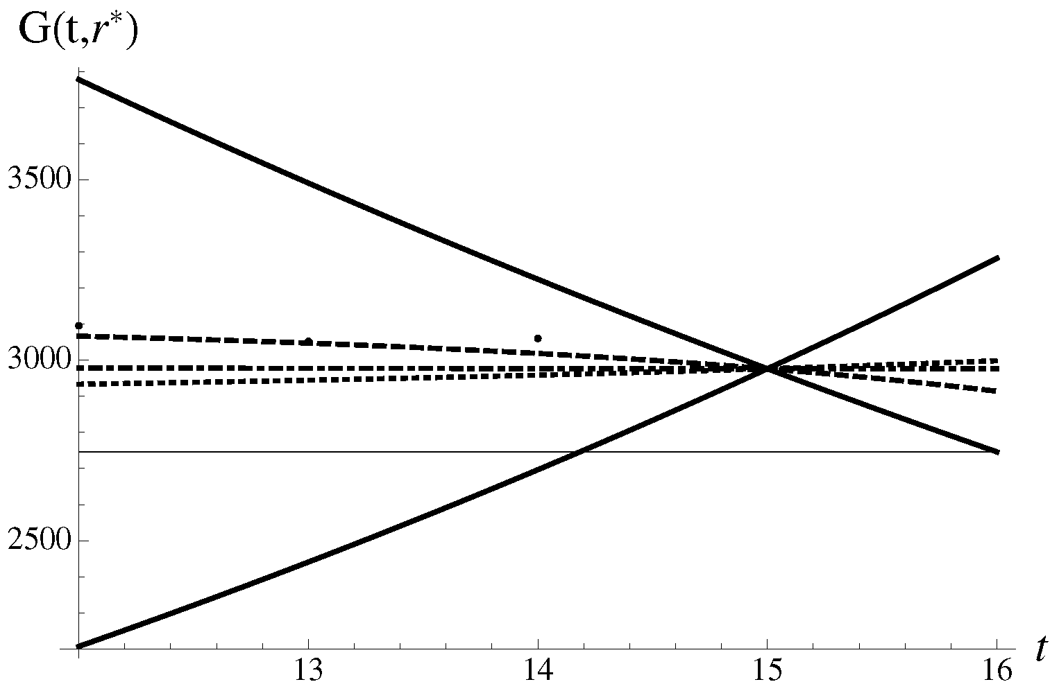
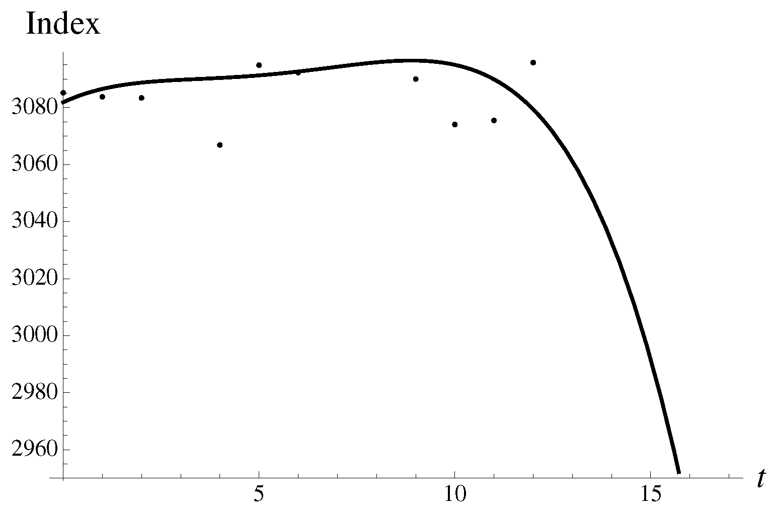
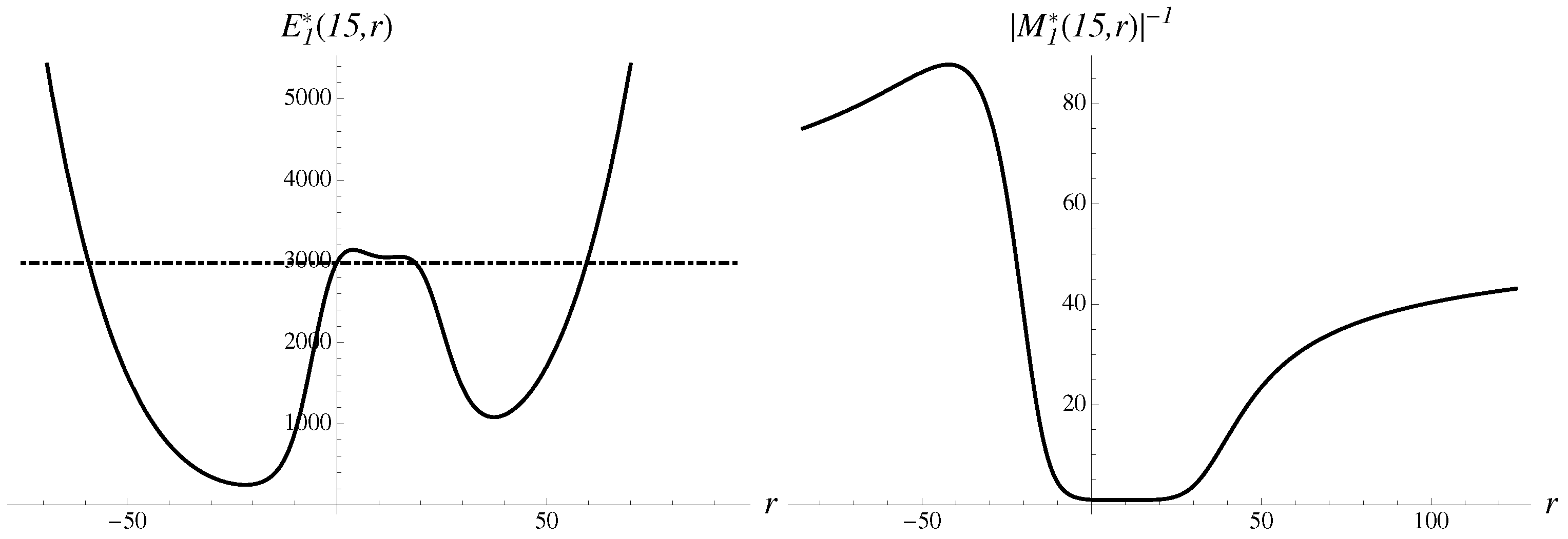
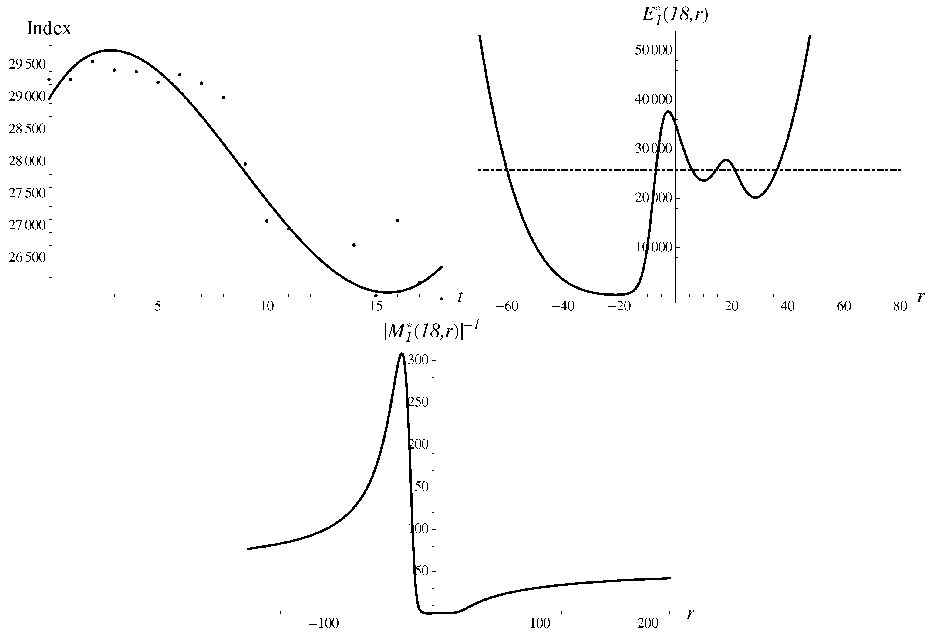
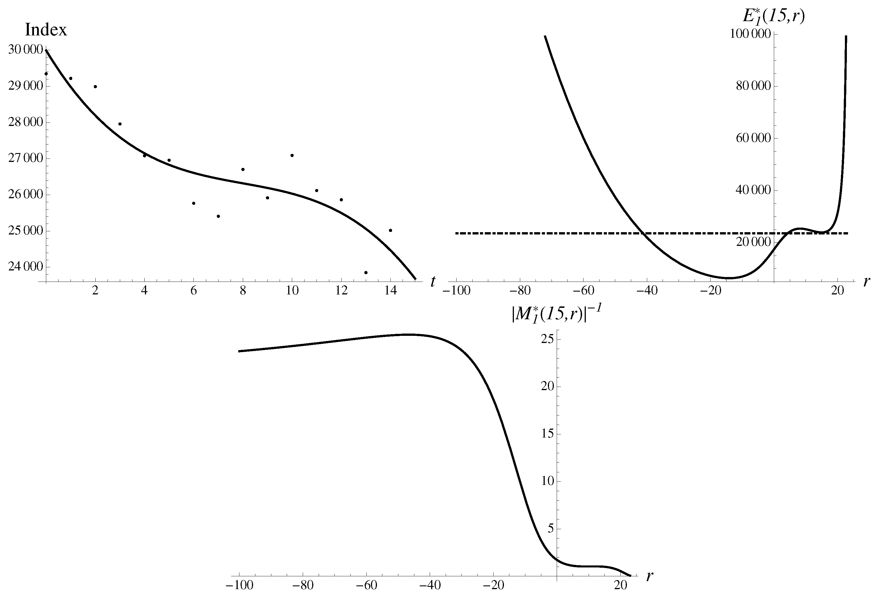
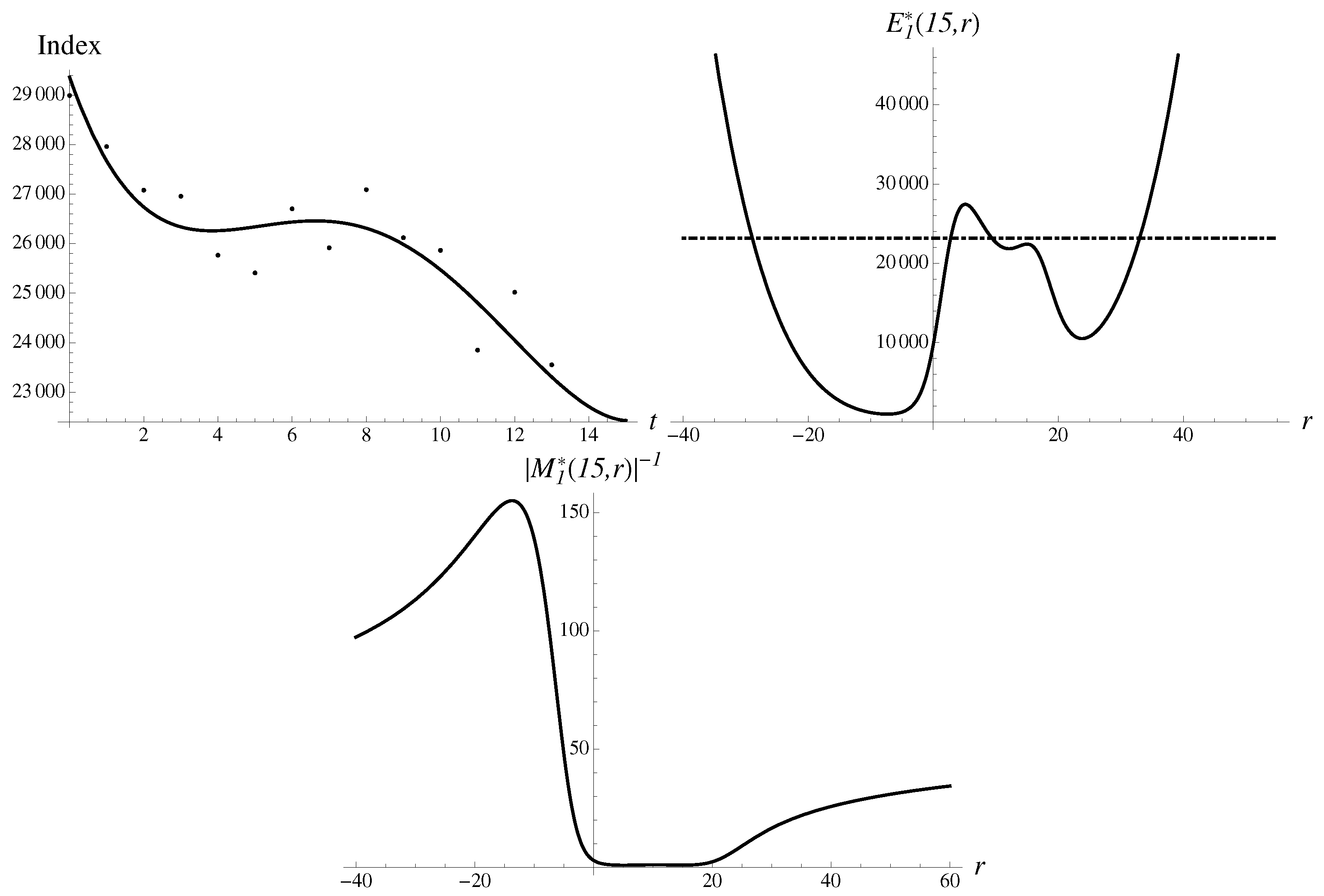
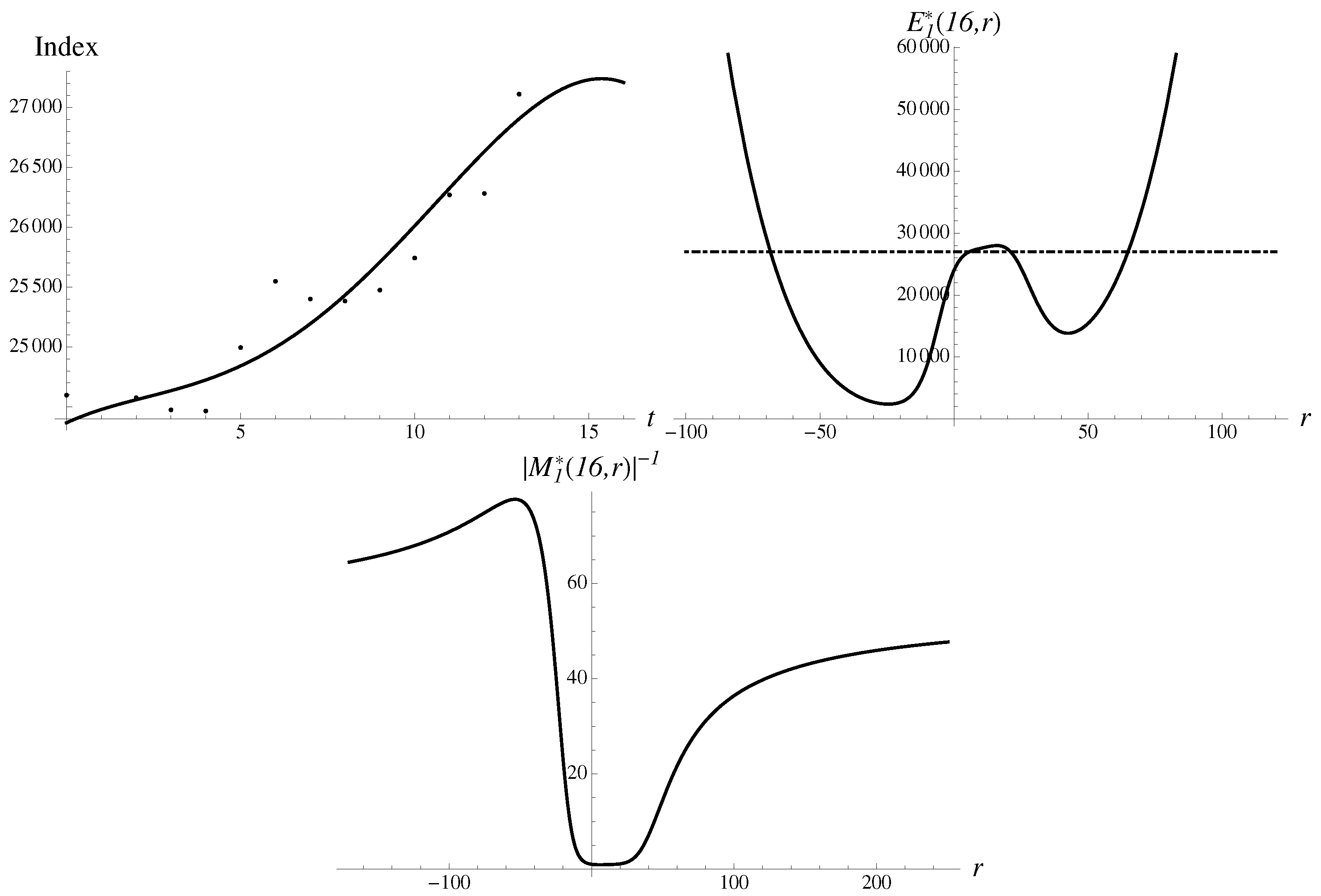
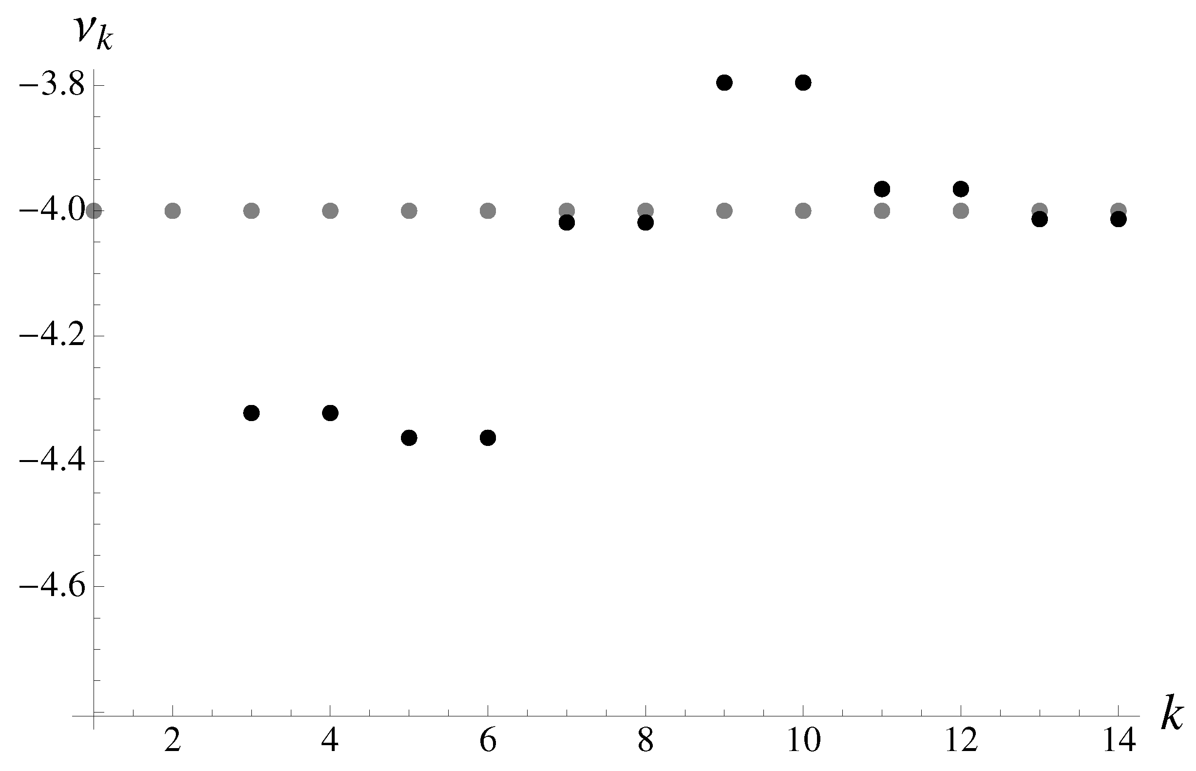
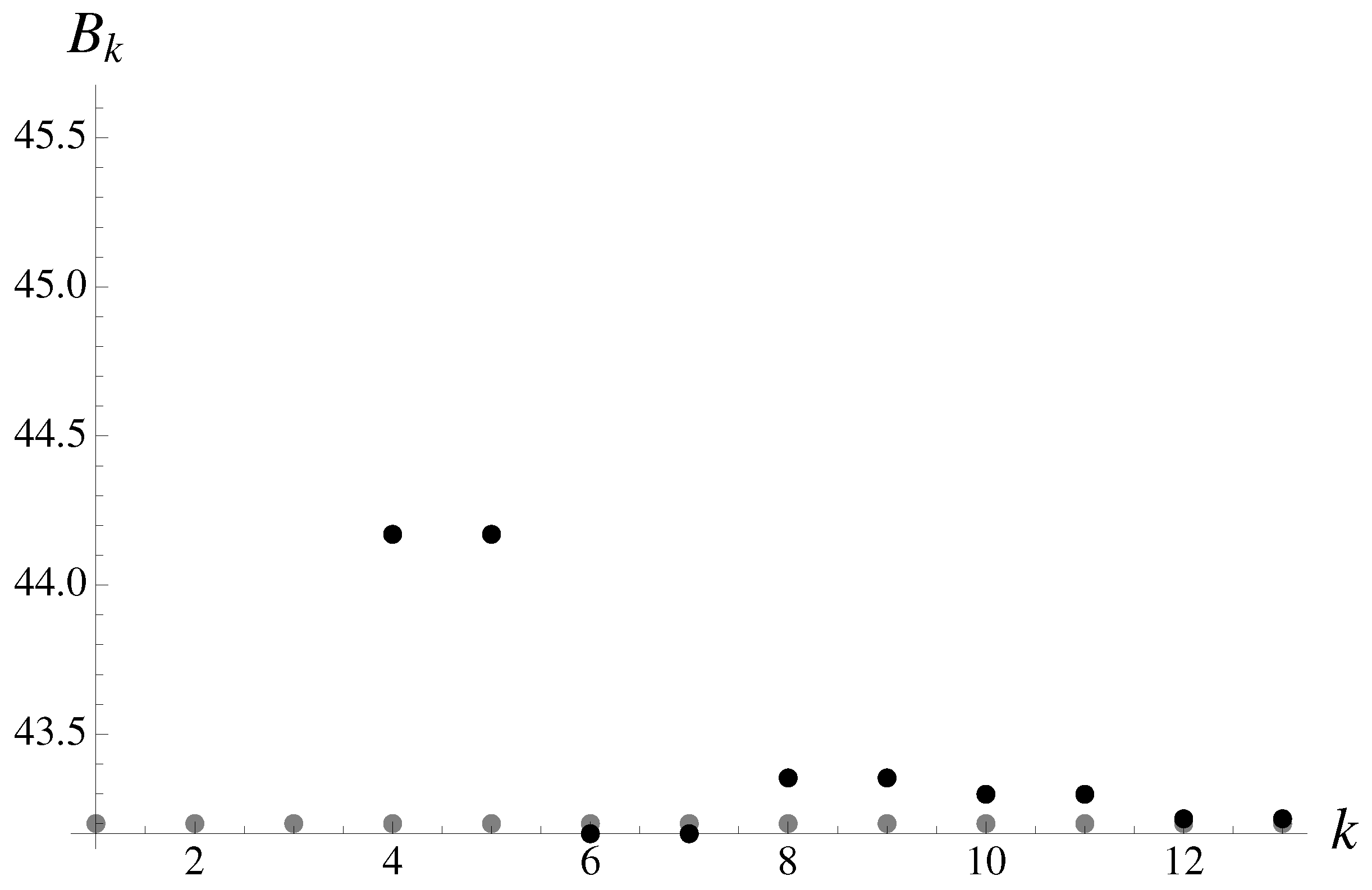
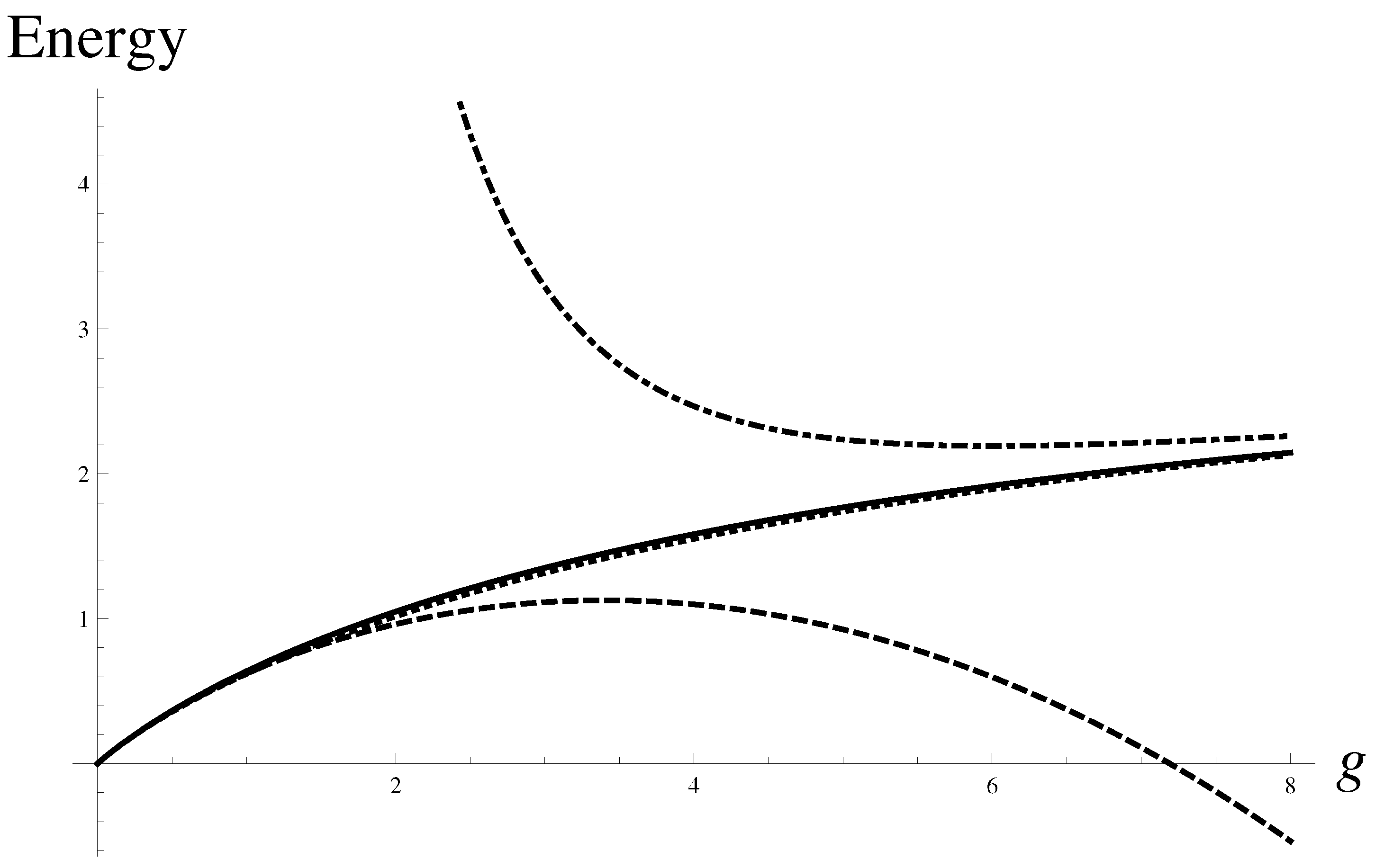
Table A1.
Ground-state energy of Lieb-Liniger model, for the varying dimensionless parameter g, in different approximations: Root approximants , , numerical data , and the Padé approximant .
Table A1.
Ground-state energy of Lieb-Liniger model, for the varying dimensionless parameter g, in different approximations: Root approximants , , numerical data , and the Padé approximant .
| g | ||||
|---|---|---|---|---|
| 0.00509427 | 0.00494169 | 0.00494163 | 0.00494165 | 0.00494136 |
| 0.0250691 | 0.0234269 | 0.0234247 | 0.0234254 | 0.0234125 |
| 0.100428 | 0.0875959 | 0.0875605 | 0.0875748 | 0.0872792 |
| 0.49294 | 0.361757 | 0.361368 | 0.361639 | 0.35512 |
| 1.00361 | 0.640965 | 0.640137 | 0.640920 | 0.622859 |
| 1.98395 | 1.04466 | 1.04325 | 1.04474 | 1.01247 |
| 5.122 | 1.78912 | 1.78751 | 1.78888 | 1.76111 |
| 6.02566 | 1.92249 | 1.92102 | 1.92206 | 1.89836 |
| 10.0214 | 2.31276 | 2.31188 | 2.31229 | 2.30062 |
| 20.0175 | 2.7248 | 2.72454 | 2.72458 | 2.72169 |
| 51.4117 | 3.04855 | 3.04853 | 3.04852 | 3.04825 |
| 277.602 | 3.24297 | 3.24297 | 3.24297 | 3.24927 |
It should become completely clear from observing Figure A3 that the problem of interpolation is neither simple nor superficial. The asymptotic expressions for small and large couplings have little in common with each other. Although the expansions (A18) and (A19) appear to work only for very small and very large coupling constants, the deduced approximants work rather well. More examples of interpolation with various self-similar approximants can be found in [16].
Figure A3.
The interpolation with root approximant (A20) is shown with solid line, while the Padé approximant is shown with dotted line. The weak- (dashed) and strong-coupling (dot-dashed) expansions are shown as well.
Figure A3.
The interpolation with root approximant (A20) is shown with solid line, while the Padé approximant is shown with dotted line. The weak- (dashed) and strong-coupling (dot-dashed) expansions are shown as well.

References
- Baxter, R.J. Exactly Solved Models in Statistical Mechanics; Academic Press: Cambridge, MA, USA, 1989. [Google Scholar]
- Izyumov, Y.A.; Skryabin, Y.N. Statistical Mechanics of Magnetically Ordered Systems; Springer: Berlin, Germany, 1988. [Google Scholar]
- Mendoza-Hernández, J.; Arroyo-Carrasco, M.; Iturbe-Castillo, M.; Chávez-Cerda, S. Laguerre-Gauss beams versus Bessel beams showdown: Peer comparison. Opt. Lett. 2015, 40, 3739–3742. [Google Scholar] [CrossRef] [PubMed]
- Taylo, J.R. Optical Solitons: Theory and Experiment; Cambridge University Press: Cambridge, UK, 1992. [Google Scholar]
- Valiulis, G.; Dubietis, A.; Piskarskas, A. Optical parametric amplification of chirped X pulses. Phys. Rev. A 2008, 77, 043824. [Google Scholar] [CrossRef]
- Baker, G.A. Padé approximant. Scholarpedia 2012, 7, 9756. [Google Scholar] [CrossRef] [Green Version]
- Hunter, J.K. Asymptotic Analysis and Singular Perturbation Theory; UC Davis: Davis, CA, USA, 2004. [Google Scholar]
- Bender, C.M.; Orszag, S.A. Advanced Mathematical Methods for Scientists and Engineers. In Asymptotic Methods and Perturbation Theory; Springer: New York, NY, USA, 1999. [Google Scholar]
- Baker, G.A.; Graves-Moris, P. Padé Approximants; Cambridge University: Cambridge, UK, 1996. [Google Scholar]
- Gluzman, S.; Yukalov, V.I. Self-similarly corrected Padé approximants for indeterminate problem. Eur. Phys. J. Plus 2016, 131, 340–361. [Google Scholar] [CrossRef] [Green Version]
- Gluzman, S.; Mityushev, V.; Nawalaniec, W. Computational Analysis of Structured Media; Academic Press: Cambridge, MA, USA, 2017. [Google Scholar]
- Dryga’s, P.; Gluzman, S.; Mityushev, V.; Nawalaniec, W. Applied Analysis of Composite Media; Elsevier: Sawston, UK, 2020. [Google Scholar]
- Andrianov, I.; Awrejcewicz, J.; Danishevs’kyy, V.; Ivankov, S. Asymptotic Methods in the Theory of Plates with Mixed Boundary Conditions; John Wiley & Sons: Hoboken, NJ, USA, 2014. [Google Scholar]
- Andrianov, I.; Shatrov, A. Padé Approximation to Solve the Problems of Aerodynamics and Heat Transfer in the Boundary Layer; IntechOpen: London, UK, 2020. [Google Scholar] [CrossRef]
- Gluzman, S.; Yukalov, V.I. Unified approach to crossover phenomena. Phys. Rev. E 1998, 58, 4197–4209. [Google Scholar] [CrossRef] [Green Version]
- Gluzman, S. Padé and Post-Padé Approximations for Critical Phenomena. Symmetry 2020, 12, 1600. [Google Scholar] [CrossRef]
- Yukalov, V.I. Interplay between Approximation Theory and Renormalization. Phys. Part. Nuclei 2019, 50, 141–209. [Google Scholar] [CrossRef] [Green Version]
- Gluzman, S.; Yukalov, V.I. Critical indices from self-similar root approximants. Eur. Phys. J. Plus 2017, 132, 535. [Google Scholar] [CrossRef] [Green Version]
- Gluzman, S.; Yukalov, V.I. Self-Similar Power Transforms in Extrapolation Problems. J. Math. Chem. 2006, 39, 47–56. [Google Scholar] [CrossRef] [Green Version]
- Yukalov, V.I.; Gluzman, S. Optimization of Self-Similar Factor Approximants. Mol. Phys. 2009, 107, 2237–2244. [Google Scholar] [CrossRef] [Green Version]
- Sauer, T. Prony’s method: An old trick for new problems. Snapshots Modern Math. Oberwolfach 2018, 4, 1–11. [Google Scholar]
- Bernstein, S. Démonstration du théoréme de Weierstrass fondée sur le calcul des probabilités. Comm. Kharkov Math. Soc. 1912, 13, 1–2. [Google Scholar]
- Cioslowski, J. Robust interpolation between weak-and strong-correlation regimes of quantum systems. J. Chem. Phys. 2012, 136, 044109. [Google Scholar] [CrossRef] [PubMed]
- Gluzman, S.; Yukalov, V.I. Effective summation and interpolation of series by self-similar root approximants. Mathematics 2015, 3, 510–526. [Google Scholar] [CrossRef] [Green Version]
- Gluzman, S.; Yukalov, V.I.; Sornette, D. Self-similar factor approximants. Phys. Rev. E 2003, 67, 026109. [Google Scholar] [CrossRef] [Green Version]
- Yukalova, E.P.; Yukalov, V.I.; Gluzman, S. Solution of differential equations by self-similar factor approximants. Ann. Phys. 2008, 323, 3074–3090. [Google Scholar] [CrossRef] [Green Version]
- Gluzman, S.; Yukalov, V.I. Self-similarly corrected Pade approximants for nonlinear equations. Int. J. Mod. Phys. B 2019, 33, 1950353. [Google Scholar] [CrossRef]
- Yukalov, V.I.; Gluzman, S. Self-similar exponential approximants. Phys. Rev. E 1998, 58, 1359–1382. [Google Scholar] [CrossRef] [Green Version]
- Gavrilov, L.A.; Gavrilova, N.S. The reliability theory of aging and longevity. J. Theor. Biol. 2001, 213, 427–453. [Google Scholar] [CrossRef] [PubMed] [Green Version]
- Gluzman, S. Market crashes and time-translation invariance. Quant. Tech. Anal. 2020. [Google Scholar] [CrossRef]
- Yukalov, V.I. Statistical mechanics of strongly nonideal systems. Phys. Rev. A 1990, 42, 3324–3334. [Google Scholar] [CrossRef] [PubMed]
- Yukalov, V.I. Method of self-similar approximations. J. Math. Phys. 1991, 32, 1235–1239. [Google Scholar] [CrossRef]
- Yukalov, V.I. Stability conditions for method of self-similar approximations. J. Math. Phys. 1992, 33, 3994–4001. [Google Scholar] [CrossRef]
- Drygaś, P.; Filishtinski, L.A.; Gluzman, S.; Mityushev, V. Conductivity and elasticity of graphene-type composites. In 2D and Quasi-2D Composite and Nano Composite Materials, Properties and Photonic Applications; McPhedran, R., Gluzman, S., Mityushev, V., Rylko, N., Eds.; Elsevier: Amsterdam, The Netherlands, 2020; Chapter 8; pp. 193–231. [Google Scholar]
- Malevich, A.E.; Mityushev, V.V.; Adler, P.M. Stokes flow through a channel with wavy walls. Acta Mech. 2006, 182, 151–182. [Google Scholar] [CrossRef]
- Brading, K.; Castellani, E.; Teh, N. Symmetry and symmetry breaking. In The Stanford Encyclopedia of Philosophy, Winter 2017 Edition; Zalta Edward, N., Ed.; SEP: Standford, CA, USA, 2017. [Google Scholar]
- Ma, S. Theory of Critical Phenomena; Benjamin: London, UK, 1976. [Google Scholar]
- Andersen, J.V.; Gluzman, S.; Sornette, D. General framework for technical analysis of market prices. Europhys. J. B 2000, 14, 579–601. [Google Scholar]
- Fliess, M.; Join, C. A mathematical proof of the existence of trends in financial time series. arXiv 2009, arXiv:0901.1945v1. [Google Scholar]
- Peters, O. Optimal leverage from non-ergodicity. Quant. Fin. 2011, 11, 593–602. [Google Scholar] [CrossRef] [Green Version]
- Peters, O.; Klein, M. Ergodicity breaking in geometric Brownian motion. Phys. Rev. Lett. 2013, 110, 100603. [Google Scholar] [CrossRef] [Green Version]
- Peters, O.; Gell-Mann, M. Evaluating gambles using dynamics. Chaos 2016, 26, 023103. [Google Scholar] [CrossRef]
- Taleb, N.N. Statistical Consequences of Fat Tails (Technical Incerto Collection). 2020. Available online: https://www.academia.edu/download/59794771/Technical_Incerto_Vol_1.pdf (accessed on 26 October 2020).
- Sacha, K. Modeling spontaneous breaking of time-translation symmetry. Phys. Rev. A 2015, 91, 033617. [Google Scholar] [CrossRef] [Green Version]
- Yukalov, V.I.; Gluzman, S. Weighted fixed points in self-similar analysis of time series. Int. J. Mod. Phys. B 1999, 13, 1463–1476. [Google Scholar] [CrossRef] [Green Version]
- Hayek, F.A. The use of knowledge in society. Am. Econ. Rev. 1945, 35, 519–530. [Google Scholar]
- Mann, A. Market forecasts. Nature 2017, 538, 308–310. [Google Scholar] [CrossRef] [PubMed] [Green Version]
- Soros, G. Fallibility, reflexivity, and the human uncertainty principle. J. Econ. Methodol. 2013, 20, 309–329. [Google Scholar] [CrossRef] [Green Version]
- Gluzman, S.; Yukalov, V.I. Renormalization group analysis of October market crashes. Mod. Phys. Lett. B 1998, 12, 75–84. [Google Scholar] [CrossRef] [Green Version]
- Buchanan, M. What has econophysics ever done for us? Nat. Phys. 2013, 9, 317. [Google Scholar] [CrossRef] [Green Version]
- Shiller, R.J. Narrative economics. Am. Econ. Rev. 2017, 107, 967–1004. [Google Scholar] [CrossRef]
- Arnold, V.I. Mathematical Methods of Classical Mechanics; Springer: Berlin, Germany, 1989. [Google Scholar]
- Zhang, Q.; Zhang, Q.; Sornette, S. Early warning signals of financial crises with multi-scale quantile regressions of log-periodic power law singularities. PLoS ONE 2016, 11, e0165819. [Google Scholar] [CrossRef]
- Gluzman, S.; Yukalov, V.I. Booms and crashes of self-similar markets. Mod. Phys. Lett. B 1998, 12, 575–587. [Google Scholar] [CrossRef] [Green Version]
- Bogoliubov, N.N.; Shirkov, D.V. Quantum Fields; Benjamin-Cummings Pub. Co.: San Francisco, CA, USA, 1982. [Google Scholar]
- Shirkov, S.V. The renormalization group, the invariance principle, and functional self-similarity. Sov. Phys. Dokl. 1982, 27, 197–199. [Google Scholar]
- Kröger, H. Fractal geometry in quantum mechanics, field theory and spin systems. Phys. Rep. 2000, 323, 81–181. [Google Scholar] [CrossRef]
- Adamou, A.; Berman, Y.; Mavroyiannisz, D.; Peters, O. Microfoundations of Discounting. arXiv 2019, arXiv:1910.02137v2. [Google Scholar] [CrossRef] [Green Version]
- Bougie, J.; Gangopadhyaya, A.; Mallow, J.; Rasinariu, C. Supersymmetric quantum mechanics and solvable models. Symmetry 2012, 4, 452–473. [Google Scholar] [CrossRef] [Green Version]
- Gluzman, S.; Sornette, D. Log-periodic route to fractal functions. Phys. Rev. E 2002, 65, 036142. [Google Scholar] [CrossRef] [PubMed] [Green Version]
- Lynch, C.; Mestel, B. Logistic model for stock market bubbles and anti-bubbles. Int. J. Theor. Appl. Financ. 2017, 20, 1750038. [Google Scholar] [CrossRef] [Green Version]
- Yukalov, V.I.; Gluzman, S. Extrapolation of power series by self-similar factor and root approximants. Int. J. Mod. Phys. B 2004, 18, 3027–3046. [Google Scholar] [CrossRef] [Green Version]
- Duguet, T.; Sadoudi, J. Breaking and restoring symmetries within the nuclear energy density functional method. J. Phys. G Nucl. Part. Phys. 2010, 37, 064009. [Google Scholar] [CrossRef] [Green Version]
- Lei, Y.C.; Zhang, S.Y. Features and partial derivatives of Bertalanffy-Richards growth model in forestry. Nonlinear Anal. Model. Control 2004, 9, 65–73. [Google Scholar] [CrossRef]
- Richards, F.J. A flexible growth function for empirical use. J. Exp. Bot. 1959, 10, 290–301. [Google Scholar] [CrossRef]
- Gluzman, S.; Karpeev, D. Perturbative expansions and critical phenomena in random structured media. In Modern Problems in Applied Analysis; Drygaś, P., Rogosin, S., Eds.; Birkhauser: Basel, Switzerland, 2017; pp. 117–134. [Google Scholar]
- Sandhu, R.; Georgiou, T.; Tannenbaum, A. Market Fragility, Systemic Risk, and Ricci Curvature. arXiv 2015, arXiv:1505.05182v1. [Google Scholar]
- Boudoukh, J.; Feldman, R.; Kogan, S.; Richardson, M. Which News Moves Stock Prices? A Textual Analysis. NBER Working Paper No. 18725. January 2012. Available online: https://www.nber.org/papers/w18725 (accessed on 26 October 2020).
- Harmon, D.; Lagi, M.; de Aguiar, M.A.M.; Chinellato, D.D.; Braha, D.; Epstein, I.R.; Bar-Yam, Y. Anticipating economic market crises using measures of collective panic. PLoS ONE 2015, 10, e0131871. [Google Scholar] [CrossRef] [PubMed]
- Bernanke, B.S.; Gertler, M.; Watson, M. Systematic monetary policy and the effects of oil price shocks. Brook. Pap. Econ. Act. 1997, 1, 91–157. [Google Scholar] [CrossRef] [Green Version]
- Kleinert, H. Vortex origin of tricritical point in Ginzburg–Landau theory. Europhys. Lett. 2006, 74, 889–895. [Google Scholar] [CrossRef] [Green Version]
- Adler, P.M. Porous Media. Geometry and Transport, 2nd ed.; Butterworth-Heinemann: New York, NY, USA, 1992. [Google Scholar]
- Pozrikidis, C. Creeping flow in two-dimensional channel. J. Fluid Mech. 1987, 180, 495–514. [Google Scholar] [CrossRef]
- Lieb, E.H.; Liniger, S. Exact analysis of an interacting Bose gas: The general solution and the ground state. Phys. Rev. 1963, 13, 1605–1616. [Google Scholar] [CrossRef]
- Yukalov, V.I.; Girardeau, M.D. Fermi-Bose mapping for one-dimensional Bose gases. Laser Phys. Lett. 2005, 2, 375–382. [Google Scholar] [CrossRef] [Green Version]
- Yukalov, V.I.; Yukalova, E.P.; Gluzman, S. Extrapolation and interpolation of asymptotic series by self-similar approximants. J. Math. Chem. 2010, 47, 959–983. [Google Scholar] [CrossRef] [Green Version]
- Dunjko, V.; Olshanii, M. Available online: http://physics.usc.edu/olshanii/DIST/ (accessed on 26 October 2020).
Figure 1.
All Gompertz approximants corresponding to the discrete spectrum, i.e., solutions to (56) are shown. The most stable downward and less stable upward solutions are shown with solid lines. Three additional solutions are shown as well. The solution shown with the dashed line is closest to the data. The “no-change”, practically flat solution, is shown with a dot-dashed line. Another solution, corresponding to moderate growth, is shown with a dotted line. The level is shown with black line. Several historical data points are shown as well.

Figure 2.
COVID-19, Shanghai Composite, 3 February 2020. Fourth-order regression is shown against data points.
Figure 2.
COVID-19, Shanghai Composite, 3 February 2020. Fourth-order regression is shown against data points.

Figure 3.
Shanghai Composite, 3 February 2020. Calculations with fourth-order regression. The inverse multiplier is shown as a function of the origin r at , . The first-order approximant is shown in a separate figure. Level is shown as well, with dot-dashed line.
Figure 3.
Shanghai Composite, 3 February 2020. Calculations with fourth-order regression. The inverse multiplier is shown as a function of the origin r at , . The first-order approximant is shown in a separate figure. Level is shown as well, with dot-dashed line.

Figure 4.
Black Monday I. Pattern in DJ Industrial index preceding 9 March 2020 Non-monotonous decay pattern reminds of a hockey stick. Fourth-order regression is shown against data points. The inverse multiplier is shown as a function of the origin r at , . The first-order approximant is shown in separate figures. Level 25,864.8 is shown with a dot-dashed line.

Figure 5.
Black Thursday. Pattern in DJ Industrial index preceding 12 March 2020. Monotonous decay pattern. Third-order regression is shown against data points. The inverse multiplier is shown as a function of the origin r at , . The first-order approximant is shown in separate figures. Level 23,553.2 is shown with a dot-dashed line.

Figure 6.
Black Monday II. Pattern in DJ Industrial index preceding 16 March 2020. Non-monotonous decay pattern. Fourth-order regression is shown against data points. The inverse multiplier is shown as a function of the origin r at , . The first-order approximant is shown in separate figures. Level 23,185.6 is shown with a dot-dashed line.

Figure 7.
Temporal bubble in Dow Jones Industrial index, preceding mini-crash of 11 June 2020. Fourth-order regression is shown against data points. The first-order approximant and multiplier are shown in separate figures. Level 26,990 is shown with a dot-dashed line.
Figure 7.
Temporal bubble in Dow Jones Industrial index, preceding mini-crash of 11 June 2020. Fourth-order regression is shown against data points. The first-order approximant and multiplier are shown in separate figures. Level 26,990 is shown with a dot-dashed line.

Table 1.
Walls can touch (b = 1/2). The problems described in Appendix A and Appendix A.1. Critical indices for the permeability obtained from the optimization conditions (41). There is rather good numerical convergence to the number .
Table 1.
Walls can touch (b = 1/2). The problems described in Appendix A and Appendix A.1. Critical indices for the permeability obtained from the optimization conditions (41). There is rather good numerical convergence to the number .
| 2.18445 | 2.39678 | |
| 2.68311 | 2.52028 | |
| 2.48138 | 2.49208 | |
| 2.49096 | 2.49692 | |
| 2.5012 | 2.49982 | |
| 2.49935 | 2.499 | |
| 2.49861 | 2.49861 |
Table 2.
Walls can touch (b = 1/4). The problems described in the Appendix A and Appendix A.2. Critical indices are found from the optimization conditions (41). There is a good numerical convergence of the sequences to the value .
Table 2.
Walls can touch (b = 1/4). The problems described in the Appendix A and Appendix A.2. Critical indices are found from the optimization conditions (41). There is a good numerical convergence of the sequences to the value .
| 2.34165 | 2.452 | |
| 2.52463 | 2.50542 | |
| 2.4976 | 2.49933 | |
| 2.49941 | 2.50004 | |
| 2.50028 | 2.50033 | |
| 2.50032 | 2.50036 | |
| 2.50041 | 2.50041 |
Table 3.
Walls can not touch. Case of b = 1/2. Critical indices for the permeability for the problems in Appendix A and Appendix A.3, obtained from the optimization conditions . The sequences demonstrate reasonably good numerical convergence to the value .
Table 3.
Walls can not touch. Case of b = 1/2. Critical indices for the permeability for the problems in Appendix A and Appendix A.3, obtained from the optimization conditions . The sequences demonstrate reasonably good numerical convergence to the value .
| −6 | −4.36 | |
| −4.04 | −4.1 | |
| n.a. | −4.13 | |
| −4.09 | −4.05 | |
| −3.97 | −4.03 | |
| n.a. | −4.08 | |
| −3.94 | −3.94 |
Publisher’s Note: MDPI stays neutral with regard to jurisdictional claims in published maps and institutional affiliations. |
© 2020 by the author. Licensee MDPI, Basel, Switzerland. This article is an open access article distributed under the terms and conditions of the Creative Commons Attribution (CC BY) license (http://creativecommons.org/licenses/by/4.0/).
Share and Cite
MDPI and ACS Style
Gluzman, S. Nonlinear Approximations to Critical and Relaxation Processes. Axioms 2020, 9, 126. https://0-doi-org.brum.beds.ac.uk/10.3390/axioms9040126
AMA Style
Gluzman S. Nonlinear Approximations to Critical and Relaxation Processes. Axioms. 2020; 9(4):126. https://0-doi-org.brum.beds.ac.uk/10.3390/axioms9040126
Chicago/Turabian StyleGluzman, Simon. 2020. "Nonlinear Approximations to Critical and Relaxation Processes" Axioms 9, no. 4: 126. https://0-doi-org.brum.beds.ac.uk/10.3390/axioms9040126
Note that from the first issue of 2016, this journal uses article numbers instead of page numbers. See further details here.