
A Mathematical Modeling and Analysis Method for the Kinematics of a Maglev Train


1
College of Intelligence Science and Technology, National University of Defense Technology, Changsha 410073, China
2
Hunan Provincial Key Laboratory of Electromagnetic Levitation and Propulsion Technology, Changsha 410073, China
*
Author to whom correspondence should be addressed.
Machines 2022, 10(5), 398; https://0-doi-org.brum.beds.ac.uk/10.3390/machines10050398
Submission received: 21 March 2022
/
Revised: 12 May 2022
/
Accepted: 17 May 2022
/
Published: 19 May 2022
(This article belongs to the Section Vehicle Engineering)
Abstract
:In recent years, more and more countries are paying attention to maglev transportation because of its outstanding advantages. However, because the structure of a maglev train is more complex than a wheel-rail train, there is no systematic theory method for kinematic modeling of a maglev vehicle. Based on the screw theory and the product of exponentials (PoE) formula in the field of open-chain robotics, this paper presents a method of kinematic mathematical modeling and analysis for a maglev train and track. By analyzing the characteristics of the closed chain running mechanism of a maglev train, the kinematic mathematical model of a maglev train and track is established, and the motion state of each moving part of the vehicle on a typical track is calculated and analyzed. At last, compared with the results of experiment, the correctness of modeling method proposed in this paper is verified.
1. Introduction
A maglev train realizes suspension, guidance and propulsion through non-contact electromagnetic force. Compared with the wheel-rail train, it has the advantages of being faster, lower vibration and noise, non-contact wear and tear, and stronger climbing and turning ability, which makes the maglev train an important direction of rail transit in the future. Germany, Japan, America, China, and other countries have carried out active research on maglev transportation technology. In China, with the operation of the Beijing S1 Maglev Commercial Line and the Changsha Maglev Express Line, maglev traffic presents a rapid development tendency.
In traditional wheel-rail train, each vehicle is usually supported by two bogies. Two points determine a straight line, so the kinematics of the running mechanism of a wheel-rail train is relatively simple and do not need systematic theoretical modeling [1]. In contrast, the carriage of a maglev train is supported by multiple suspension frames. The motion states of the suspension frames are different due to vehicle position and track-line shape, which is much more complex than that of wheel rail train [2,3]. Therefore, the kinematic analysis method of wheel-rail train is not suitable for a maglev train. Now, the kinematic modeling of maglev train is still at the level of simple measurement from the CAD and equivalent estimation, which restricts the development of maglev transportation technology. It is urgent to establish a complete and systematic method of kinematic modeling and analysis.
In mechanism kinematic modeling methods, the D-H transformation proposed by Denavit and Hartenberg [4,5] is a common method. However, the motion equation and the Jacobian matrix established by D-H transformation depend on the selection of a coordinate system on each linkage [6,7], which leads to the loss of generality of analysis results. In addition, in non-straight tracks, such as transition curve and circular curve [8,9,10], the D-H transformation method can only establish an approximate mathematical model and cannot give the accurate solution [11]. Therefore, in this paper, screw transformation and exponential mapping [5] are used to build a kinematic model of a running mechanism and track line, to study the ability of running mechanism adapting track lines, or to study the rationality of the design parameters while the track and vehicle body parameters are given. This paper presents a systematic, accurate, efficient and general kinematic mathematical modeling and analysis method for a maglev train.
The article [12] only established a kinematic analysis method for anti-rolling beams, which are part of the suspension frame, and did not involve the complex kinematics of vehicle running mechanism on tracks. In this paper, we built a comprehensive kinematic mathematical modeling of the vehicle and track line: a model of the secondary system, which is the main part of running mechanism of vehicle; a model of the circular curve track and the relative position of the vehicle to the track line. The proposed method is applicable to both a TR high-speed maglev train and mid-low speed maglev train. Here, only the mid–low-speed maglev train is discussed because the space of the article is limited.
2. Forward Kinematic Modeling of Suspension System
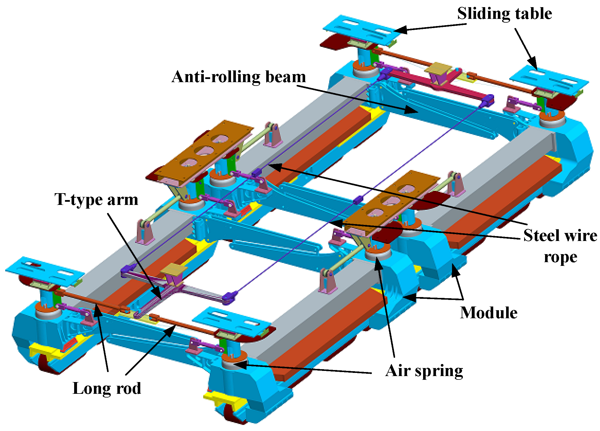
The running mechanism of a maglev train mainly includes suspension frame, secondary system, auxiliary steering mechanism, etc. to realize the functions of suspension, guidance and traction. The structure of running mechanism is shown in Figure 1. Therefore, the kinematic model can be built in two levels: suspension frame kinematics and secondary system kinematics. The left and right modules of the suspension frame are constrained by track and move along the track; its kinematics mainly analyze the movement of anti-rolling beams and hanger rods inside the same suspension frame [12]. The kinematic modeling of secondary system mainly analyzes the state of secondary system components between vehicle body and suspension frame when it moves along the track. This paper focuses on the kinematic modeling and analysis of a secondary system and a circular curve track.
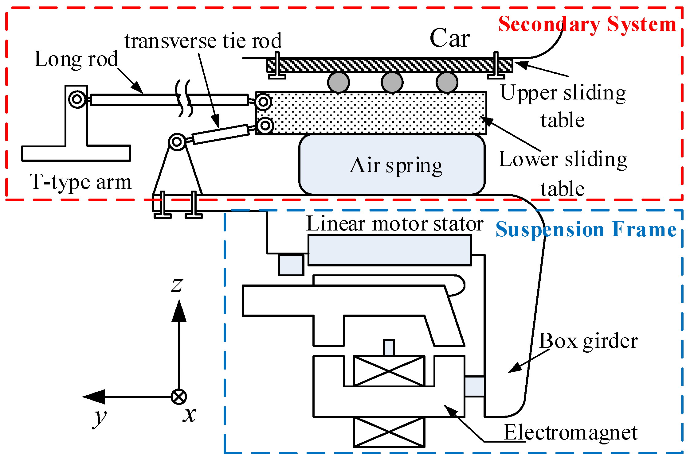
The secondary system of mid–low-speed maglev train consists of sliding tables, air springs, transverse tie rods, longitudinal push rods and a steering mechanism. These components constrain the relative motion between the suspension frame and the vehicle body while transmitting suspension, guidance, traction and braking forces. From the overall vehicle, the secondary system in a suspension frame and the vehicle body form a closed-chain mechanism with a left–right symmetrical structure. So, it is reasonable to establish a kinematics equation of only one side of the secondary system as an open-chain structure. The structure is shown in Figure 2. In modeling, the steering mechanism with redundant constraints and the longitudinal push rods are ignored, and the definition of open-chain degrees of freedom and screw axes structure are shown in Figure 3.
The reference coordinate system is fixed on the support of the transverse tie rod. The terminal coordinate system of the series mechanism is fixed at the center of the upper sliding table on the vehicle body, and its initial posture is the same as . Additionally, is the length of the transverse tie rod, which is the distance between screw axis and ; is the length from the transverse tie rod to the lower sliding table, which is the distance from screw axis to . The kinematics equation is established by screw theory [13]. The twist axes and the degree of freedom of the joints are defined as follows:
- 1.
- The screw axis is a rotational degree of freedom in the x-negative direction between the transverse tie rod and its support. This movement is generated by the change in height of air spring.
- 2.
- The screw axis is a rotational degree of freedom in the z-direction between the transverse tie rod and its support. This motion is generated by x-direction translation of suspension module to vehicle body or yaw motion.
- 3.
- The screw axis is a rotational degree of freedom in the y-negative direction between the transverse tie rod and its support. This motion is generated by module’s pitching motion relative to the vehicle body about the y-axis.
- 4.
- The screw axis is a rotational degree of freedom in the x-negative direction between the transverse tie rod and the lower sliding table. This movement is generated by the change in the height of the air spring. In addition, the motion around the y-axis is an internal freedom here, which is ignored in modeling.
- 5.
- The screw axis is a rotational degree of freedom in the z-direction between the transverse tie rod and the lower sliding table. This motion is also generated by x-direction translation of the suspension module to the vehicle body or yaw motion.
- 6.
- The screw axis is a translational degree of freedom in the y-negative direction, describing the translational motion of the sliding table. This motion is generated by the lateral translation of the suspension module to the vehicle body.
It can be seen from the above definition that open-chain model of a secondary system of a mid–low-speed maglev train has six degrees of freedom, including five rotations and one translation. According to the coordinate system above, we can get the feature point vectors on the corresponding rotation axis, and then obtain the screw coordinate . According to the screw coordinate, we can get the exponential mapping of each vector, and then obtain the forward kinematic model of the secondary system. The specific solution process is given as follows.
—the unit rotation axis; —the any point on rotation axis; —the linear velocity, and ; —the rotation angle or translation distance of the joint.
According to Figure 3, the feature point vectors on the six screw axes can be given as:
The exponential mapping of screw coordinates is:
The forward kinematics equation of suspension module to vehicle body is:
where, is the initial pose of upper sliding table on vehicle body relative to on suspension module [14], which can be obtained from the coordinate system in Figure 3:
and is also a 4 × 4 matrix, and its parameter representation is shown in Equation (3).
By combining Equations (1) and (2), we can obtain the specific value of Equation (3) as follows, where , .
If the motion of the joints in secondary system is known, the pose of suspension module relative to vehicle body can be calculated by the kinematic model above. On the contrary, if the relative pose between the vehicle and the suspension module is known, the state of each component in the secondary system can also be calculated using the inverse kinematic model. The proposed kinematic model can be used as a basic tool for design, analysis and verification of the secondary system of a maglev train.
3. Inverse Kinematics Solution of Secondary System
There are two methods to get an inverse kinematics solution from the product of the exponentials formula of the forward kinematics equation and the initial conditions of the secondary system: the sub-problem method of exponential mapping [6,7] and the inverse transformation method of robot kinematics solution [5]. The two methods have a basic idea, which is to simplify exponential equation so that the concise terms on both sides are equal, and then get joint motions of the moving mechanism. Obtaining an analytical solution for the inverse kinematic model is a skilled job and requires certain conditions. The following is derivation process of inverse kinematics solution from the forward kinematics Equation (2) of the secondary system.
Assume that the pose matrix of upper slide coordinate system , relative to reference coordinate system , is:
In Equation (4), each element in is known. (The component state is known). Using as the input of kinematics equation, we get:
The transformation of the above equation is:
The matrix on the right side of Equation (6) is known, and the left side is a function matrix of –. Transforming Equation (6), we get:
In Equation (7), selecting the first three rows of elements in the fourth column to be equal, we can get Equation (8):
The three equations in Equation (8) are independent of each other, from which we can get three variables , , shown in Equations (9)–(11).
, and are shown in Equation (12).
Now, all elements on the right side of Equation (7) have become known quantities. Observing the matrix on the left side of Equation (7) and making the second element in the first row equal, then we can get , as follows:
The first column elements in the first row is equal in Equation (7); then, we can obtain as follows:
Or can be obtained by dividing the first element and the third element in the first row:
In Equation (14), is generally a small angle, so the denominator will not be zero. However, Equation (14) contains less information and is greatly affected by truncation error. Equation (15) contains more information, but it is necessary to avoid a situation in which and are zero at the same time.
According to the second element of the second line and the second element of the third line in Equation (7), we can obtain as follows:
Or can be:
These two methods of solving have the same principle as the above method of solving .
So far, we have obtained the rotational or translational motion of six degrees of freedom – in a secondary system from the relative pose of the upper sliding table and suspension module.
4. The Relative Pose of Vehicle to Circular Curve Track
The constraint of track to vehicle is achieved by electromagnetic force of an on-board electromagnet. The electromagnet is a linear rigid body, while the track is often a curve. Therefore, except that an electromagnet on straight track is parallel to the track, there is some dislocation between the electromagnet and the track on other curved tracks. In this paper, by establishing the mathematical model of the space curve and analyzing the vehicle/track pose, the motion state of the maglev train can be scientifically analyzed.
4.1. Parametric Description of Circular Curve
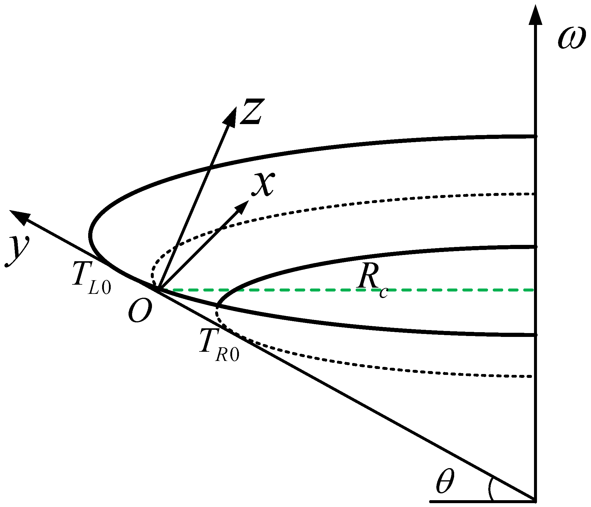
The circular curve has a constant radius and is a type of horizontal curve. The flat of circular curve track is a conical surface in space, which is generally described by two parameters: cross-slope angle and curve radius . From the perspective of the space, the centerline and inner and outer rails of circular curve are all plane curves. However, due to the existence of superelevation (cross slope angle ), a flat circular curve becomes a conical surface instead of a cylinder. Therefore, the circular curve track can be regarded as a conical surface with rotation axis passing through the center of the centerline and perpendicular to the ground. The generatrix length of the cone is with the angle to ground; the track is located on this conical surface. This spatial relationship of circular curves can be described by screw transformation. The sketch map of the circular curves track is shown in Figure 4.
Several track coordinates systems in Figure 4 are defined as follows:
- Spatial reference coordinate system O: The origin of O is set at the start of the track centerline and conforms to the right-handed system. The x-axis is along the tangent line of the track centerline, and its positive direction is consistent with vehicle travel. The z-axis is perpendicular to the track plane, and the positive direction is upward. The y-axis is perpendicular to the centerline of the track.
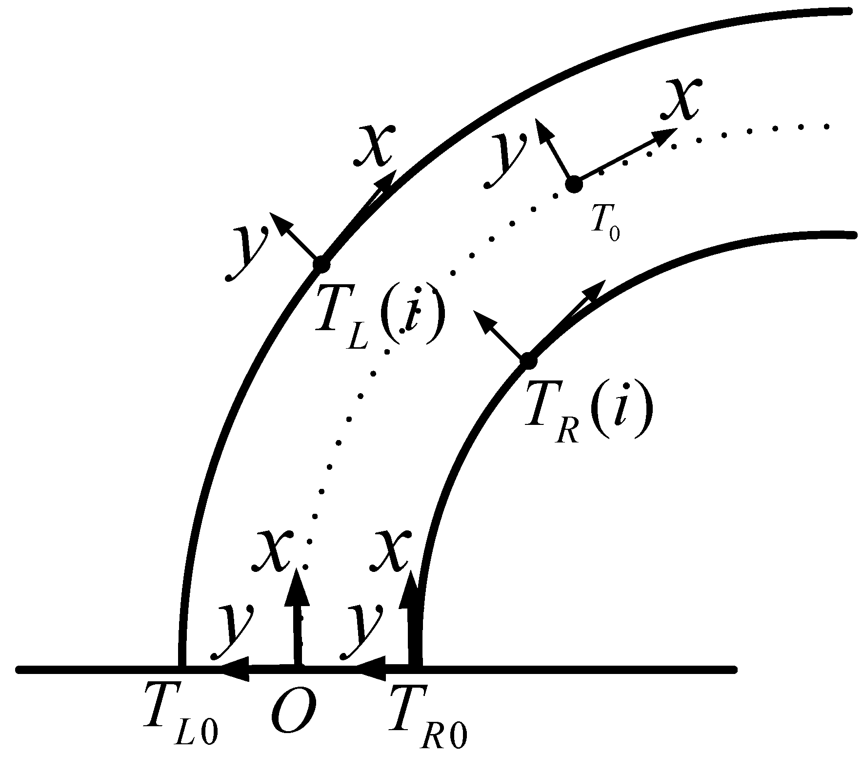
- Track starting point coordinate system and : The origins are located at the starting point of the right and left rail, respectively. Their poses are consistent with the reference coordinate system O and the distance from O is half rail-gauge. The pose of the moving coordinate system on the right running rail is consistent with .
- Track reference coordinate system : The pose of is defined as the same as the reference coordinate system O. Its origin is set on the track centerline, and the mileage from the origin O is determined according to the position of the vehicle body.
The definitions of the above coordinate systems are shown in Figure 5.
Assuming the mileage of relative to is s, the vector of rotation axis in reference coordinate system can be expressed as: . The feature point q on the rotation axis can be expressed as: , where is the radius of the right rail ( is a half-gauge less than ). According to , we can get the motion screw: .
When moves s along the right track, it is equivalent to rotating around the axis ,
and when the frame rotates clockwise around the axis, its pose matrix becomes:
In the above equation, the initial pose of the frame and are coincident, so take as follows: .Thus, the pose matrix of , determined by the mileage s, can be obtained. Similarly, the pose matrix of the left track can be obtained. The matrix is an accurate description of circular curve, which cannot be obtained by D-H transform [15]. This accurate model embodies the superiority of the screw motion mathematical method.
4.2. The Modeling of Track Coordinates on Circular Curve
When the length of electromagnet l and the distance between adjacent magnets are known, the mileage s of the reference point on the track can be obtained. Further, the corresponding coordinate systems on the right side of the track and the corresponding coordinate systems are on the vehicle body; the origin of is set on the ith motion chain on the right side of the vehicle body, and the direction of coordinate axis is consistent with . The track reference coordinate system and the vehicle reference coordinate system can be defined. The origin of is located on the central line of the vehicle body. The x-axis is along the central line of the vehicle body and points to the positive direction of the vehicle body. The z-axis is perpendicular to the vehicle body plane, and the positive direction is upward. The y-axis is perpendicular to the vehicle body central line. These coordinate systems are shown in Figure 6.
Putting at the position of . According to the relationship between mileage and rotation angle, the position vector of can be obtained from Equation (19):
In Equation (20), is the track mileage where the vehicle electromagnet coincides with the circular curve track, and there are 10 points on right track. Similarly, the pose matrix of five electromagnets can be obtained:
In Equation (21), is the track mileage at the midpoint of the electromagnet, and there are five points on the right side. Further, the pose matrix of relative to track origin coordinate is obtained as follows:
In the above equation, k is set to ensure the consistency of track coordinate-system posture and electromagnet posture at corresponding positions.
4.3. The Pose Matrix of Vehicle Reference Coordinate System Relative to Track Reference Coordinate System
The rotating sliding table1 at the intersection of suspension frame 1, 2, 4 and 5 has a constraint effect on the vehicle body. According to the pose relationship in Figure 6, we can calculate the relative pose matrix of vehicle reference coordinate system to track reference coordinate system . The vehicle is a rigid body; it is also easy to calculate the pose matrix of vehicle right-side coordinate system relative to vehicle reference coordinate system .
Thus, the pose relationship of the right vehicle coordinate system relative to the right track coordinate system is obtained:
Taking as the boundary condition of the secondary system kinematics equation, the inverse solution of kinematics can be calculated.
The track plane of a circular curve is a conical plane in space, and the vehicle body is asymmetrical on the left and right sides of the track. Therefore, it is also necessary to derive the pose relationship of the left vehicle coordinate system and left track coordinate system to comprehensively analyze the motion of a vehicle on a circular curve. The process is similar to the derivation of the right-side pose relationship above.
5. The Calculation and Test Results of Running Mechanism on Circular Curve
5.1. The Calculation Results of Running Mechanism Kinematic Model
When establishing the above-mentioned kinematics equation of secondary system, the reference coordinate system and the terminal coordinate system are set at the position of the joints for the convenience of solving the inverse solution. However, the vehicle body constrained coordinate systems , and the track coordinate systems , are not at the joint of the running mechanism. Therefore, before solving the inverse kinematics equation, several transformation matrices need to be designed to transform the vehicle rail constraint relationship to the reference system position of the inverse kinematics solution.
The space relationship of secondary systems and electromagnets with the track line is shown in Figure 7.
- , , , corresponds to the terminal coordinate system of the secondary system in Section 2, and , , , corresponds to the reference coordinate system of the secondary system.
- The meaning of several structural parameters in Figure 7 is shown as follows:: The distance from the origin of track coordinate system and on the center line of the electromagnet pole surface to the axis of the air spring (direction of the reference system);: The vertical distance from the pole surface of the electromagnet to transverse tie rod (direction of reference system);: The lateral distance from the center line of the electromagnet pole surface to the joint of transverse tie rod seat (direction of reference system);: Length of transverse tie rod. The concept has been mentioned in kinematic modeling in Section 2;: The vertical distance from the end of transverse tie rod near the air spring to the upper sliding table (direction of the reference system).
It can be directly seen in Figure 7 that the transformation matrix from to on the right suspension module is:
The transformation matrix from to on the left suspension module is:
At the same time, a pose transformation matrix is required between the left terminal coordinate system of the secondary system and the vehicle body coordinate system . The matrix is:
So, the following relationship is established for the right module:
In Equation (28), the first item on the right side is determined by Equation (25), and the second item is determined by Equation (24).
Similarly, for the left module, the following relationship is established:
In Equation (29), the first item on the right side is determined by Equation (25), and the second item is the pose relationship between the left vehicle coordinate system and the left track coordinate system ; the third item is determined by Equation (27).
By replacing the known matrix in Equation (4) in Section 3 with the matrix expressed in Equations (28) and (29), the inverse kinematics solution of secondary system can be calculated.
The parameters of the circular curve and the maglev train are shown in Table 1:
Taking the above parameters into the equation of inverse kinematics solution of the secondary system, we can get the amount of motion of 10 joints on the right side (smaller radius side of track, inner side) of the secondary system on the circular curve. The calculation results are shown in Table 2. The amount of motion of 10 joints on the left side (larger radius side of track, outer side) of the secondary system is shown in Table 3.
It can be seen from Figure 3 that the motion of the secondary system air spring is:
is the rotation angle between the transverse tie rod and its support, and the rotation axis is .
Introducing in Table 2 and Table 3 into Equation (30), respectively, the expansion and contraction quantities of air springs on the left and right side of vehicle are shown in Table 4.
The in Table 2 and Table 3 indicates the movement of the sliding table. It can be seen from the tables that the movement of the sliding table at both ends of the vehicle is larger than that of the middle sliding table, and the movement of the sliding table at the left (outer) side of the circular curve is significantly larger than that at right track. Therefore, the sliding table at both ends of the vehicle should be majorly considered when designing structure. The and reflect the rotation angle of the transverse tie rod along the vertical axis (z-axis); that is, the torsional angle of the air spring along its own axis. These two parameters are important when selecting an air spring, which involves the normal operation and service life of an air spring. Other joint movements, such as and , etc., reflect joint movement in these directions, and are important references for the design and selection of joint parameters.
5.2. The Test Results on Circular Curve
In order to verify the validity of kinematic modeling and its calculation results, a test of the motion of vehicle’s secondary system was performed on the Tangshan test line, and the motion of secondary system includes the movement of sliding table and air spring. The test site is shown in Figure 8a. The maglev train passed a circular curve with a radius of 100 m at a speed of 40 km/h under heavy load. Using the cable displacement sensor shown in Figure 8b, the moving distance of the sliding table and the height change of the air spring were tested. The layout of the measuring points is shown in Figure 9. The measuring point A4 in the figure corresponds to the right (inner) motion chain Number 1, where the displacement of the sliding table is measured by sensor S1; A3 corresponds to right motion-chain Number 2; B4 corresponds to right motion-chain Number 3, and the sliding table displacement is measured by sensor S5; B3 corresponds to right motion-chain Number 4, and the displacement of the sliding table is measured by sensor S2; A1 corresponds to left (outer) motion-chain Number 1, and the displacement of the sliding table is measured by S3; B2 corresponds to left motion-chain Number 4, and the displacement of the sliding table is measured by S4, and so on. The test results are shown in Figure 10.
Comparing the calculation results in Section 5.1 with the experimental results as shown in Table 5.
It can be seen from Table 5 that the displacement of the sliding table calculated by the kinematic model is basically the same as the displacement obtained by experimental testing, and the deviation value is caused by dynamic factors such as speed, load, track irregularity, etc., during vehicle running. The above experimental results verify the correctness of the mathematical modeling and theoretical calculation results. The displacement of the air spring is shown as Figure 11. The time period in the dotted line is the displacement curve of air springs at E3 and E4 when the vehicle is running on a circular curve; E3 and E4 correspond to Number 10 and Number 9 in Table 4, respectively. The displacement at E3 is about −16 mm and at E4 is about −4 mm, which is bigger than the theoretical values of −13.78 mm and −0.73 mm. The main reason is that the designed passing speed of the cirlular curve is 40 km/h, but it only reaches 35 km/h during the test, which leads to vehicle centrifugal force that is less than the gravity component.
6. Conclusions
Based on the screw theory and the product of exponentials formula, this paper proposes a kinematic mathematical modeling method for the running mechanism of a maglev train and its track. The proposed method can deal with the closed-chain structure of running mechanism as an open-chain structure. It is a general kinematic mathematical modeling method for a maglev train, and has higher accuracy of modeling and universality of conclusions than the D-H modeling method. The motion parameters of components of a mid–low-speed maglev train calculated from the kinematic model in this paper coincide with the test results from the experiment, which proves the validity of the kinematic modeling method based on the screw theory and the product of exponentials formula. Therefore, the paper constructs a logical and systematic modeling and analyzing method for structural design, components selection and fault analysis of a maglev train.
Author Contributions
Conceptualization, M.L., J.L., Y.J. and P.L.; data curation, J.L. and D.Z.; formal analysis, M.L. and Y.J.; funding acquisition, J.L.; investigation, M.L., Y.J., P.L. and D.Z.; methodology, M.L.; supervision, J.L. and D.Z.; writing—original draft, M.L. and J.L.; writing—review and editing, M.L. and Y.J. All authors have read and agreed to the published version of the manuscript.
Funding
This research was funded in part by the National Key Research and Development Program of China under Grant 2016YFB1200601, in part by the Major Project of Advanced Manufacturing and Automation of Changsha Science and Technology Bureau under Grant kq1804037, and in part by the Innovative Research Project for Young Teachers of College of Intelligence Science and Technology under Grant ZN2019-009.
Institutional Review Board Statement
Not applicable.
Informed Consent Statement
Not applicable.
Data Availability Statement
The original data contributions presented in the study are included in the article; further inquiries can be directed to the corresponding authors.
Conflicts of Interest
The authors declare no conflict of interest.
References
- Shang, Y. Construction and Design of EMU Vehicles; Southwest Jiaotong University Press: Chengdu, China, 2010; pp. 19–56. [Google Scholar]
- Yan, L. Development and application of the maglev transportation system. IEEE Trans. Appl. Supercond. 2008, 18, 92–99. [Google Scholar]
- Lin, G.; Sheng, X. Application and further development of Maglev transportation in China. Transp. Syst. Technol. 2018, 4, 36–43. [Google Scholar] [CrossRef]
- Xiong, Y. Science of Robotics; China Machine Press: Beijing, China, 1992; pp. 24–47. [Google Scholar]
- Cai, Z. Robotics: Principles and Applications; South and Center University Press: Changsha, China, 1988; pp. 77–108. [Google Scholar]
- Murray, R.; Li, Z.; Sastry, S. A Mathematical Introduction to Robotic Manipulation; CRC Press: Boca Raton, FL, USA, 2005; pp. 11–42. [Google Scholar]
- Yu, J.; Liu, X.; Ding, X. Mathematic Foundation of Mechanisms and Robotics; China Machine Press: Beijing, China, 2016; pp. 53–78. [Google Scholar]
- Li, J.; Sun, T.; Zhang, K. Kinematical Analysis for the Second Suspension System of the Maglev Vehicle. J. China Railw. Soc. 2007, 29, 32–38. [Google Scholar]
- Li, J.; Li, G.; Zhang, K.; Cui, P.; Zhou, D. Kinematical Analysis for the Second Suspension System of the Mid-Low-Speed Maglev Vehicle. In Proceedings of the 2013 China Automation Congress (CAC), Changsha, China, 7–8 November 2013. [Google Scholar]
- Zhang, K.; Li, J.; Chang, W. Structure Decoupling Analysis of Maglev Train Bogie. Electr. Drive Locomot. 2005, 1, 22–39. [Google Scholar]
- Li, J. The Study of Supervised Control for Coordinated Multiple Manipulators. Ph.D. Thesis, National University of Defense Technology, Changsha, China, 1999. [Google Scholar]
- Leng, P.; Li, J.; Jin, Y. Kinematics Modeling and Analysis of Mid-Low Speed Maglev Vehicle with Screw and Product of Exponential Theory. Symmetry 2019, 11, 2073–8994. [Google Scholar] [CrossRef] [Green Version]
- Zhang, Z.; Zhang, T.; Zhang, H.; Yang, J.; Cao, Y.; Jiang, Y.; Tian, D. Modeling, Kinematic Characteristics Analysis and Experimental Testing of an Elliptical Rotor Scraper Pump. Machines 2022, 10, 78. [Google Scholar] [CrossRef]
- Li, S.; Gao, P.; Yu, H.; Chen, M. Static Force Analysis of a 3-DOF Robot for Spinal Vertebral Lamina Milling. Machines 2022, 10, 29. [Google Scholar] [CrossRef]
- Zhang, G.; Li, J. Kinematics study on anti-roll boom of low-speed maglev train. J. China Railw. Soc. 2012, 34, 28–33. [Google Scholar]
Figure 1.
The suspension frame and secondary system in CMS04.

Figure 2.
One side of secondary system structure.

Figure 3.
Definition of reference coordinates and screw axis.

Figure 4.
Sketch of horizontal curve formation.

Figure 5.
Definition of track coordinate systems.

Figure 6.
Relationship between track and vehicle coordinates on circular curve.

Figure 7.
The diagram of secondary system and track constraint.

Figure 8.
Test on circular curve. (a) Maglev train running on R100m circular curve on the Tangshan test line; (b) sensor for displacement test of sliding table and air spring.
Figure 8.
Test on circular curve. (a) Maglev train running on R100m circular curve on the Tangshan test line; (b) sensor for displacement test of sliding table and air spring.

Figure 9.
The layout of measuring points and displacement sensors.

Figure 10.
Test results. (a) Displacement curve of sliding table at A1; (b) displacement curve of sliding table at A4; (c) displacement curve of sliding table at B2; (d) displacement curve of sliding table at B3.
Figure 10.
Test results. (a) Displacement curve of sliding table at A1; (b) displacement curve of sliding table at A4; (c) displacement curve of sliding table at B2; (d) displacement curve of sliding table at B3.

Figure 11.
Displacement curve of air spring at E3 and E4.


Table 1.
The parameters of the circular curve and the maglev train.
| Parameters | Value | Parameters | Value |
|---|---|---|---|
| 100.0 m | 0.4625 m | ||
| 0.501 m | |||
| D | 2.0 m | 0.765 m | |
| l | 2.65 m | 0.431 m | |
| 0.09 m | 0.441 m | ||
| 2.25 m | 0.264 m | ||
| 0.49 m |
Table 2.
The motion of joints on the right side of the vehicle’s secondary system.
| Number | (deg) | (deg) | (deg) | (deg) | (deg) | (mm) |
|---|---|---|---|---|---|---|
| 1 | −1.78 | 0.44 | 0.32 | 1.80 | −3.59 | −127.01 |
| 2 | −0.09 | 0.53 | 0.33 | 0.11 | −3.69 | −6.85 |
| 3 | 0.18 | 0.52 | 0.17 | −0.18 | −2.10 | 13.32 |
| 4 | 1.03 | 0.28 | 0.17 | −1.03 | −1.86 | 75.43 |
| 5 | 1.12 | 0.22 | 0.00 | −1.12 | −0.22 | 82.15 |
| 6 | 1.12 | −0.13 | −0.00 | −1.12 | 0.13 | 82.15 |
| 7 | 1.03 | −0.19 | −0.17 | −1.03 | 1.77 | 75.41 |
| 8 | 0.18 | −0.43 | −0.17 | −0.18 | 2.01 | 13.30 |
| 9 | −0.09 | −0.45 | −0.33 | 0.11 | 3.61 | −6.89 |
| 10 | −1.79 | −0.36 | −0.32 | 1.80 | 3.50 | −126.98 |
Table 3.
The motion of joints on the left side of the vehicle’s secondary system.
| Number | (deg) | (deg) | (deg) | (deg) | (deg) | (mm) |
|---|---|---|---|---|---|---|
| 1 | −1.73 | −0.52 | −0.31 | 1.73 | −2.58 | 130.85 |
| 2 | −0.07 | −0.60 | −0.32 | 0.06 | −2.50 | 5.07 |
| 3 | 0.20 | −0.51 | −0.16 | −0.20 | −1.04 | −14.70 |
| 4 | 1.03 | −0.27 | −0.17 | −1.03 | −1.28 | −75.47 |
| 5 | 1.12 | −0.13 | −0.00 | −1.12 | 0.13 | −82.04 |
| 6 | 1.12 | 0.22 | 0.00 | −1.12 | −0.22 | −82.04 |
| 7 | 1.03 | 0.35 | 0.17 | −1.03 | 1.19 | −75.48 |
| 8 | 0.20 | 0.60 | 0.16 | −0.20 | 0.95 | −14.71 |
| 9 | −0.07 | 0.69 | 0.32 | 0.06 | 2.41 | 5.04 |
| 10 | −1.73 | 0.61 | 0.31 | 1.73 | 2.49 | 130.89 |
Table 4.
The motion of air spring on right and left side of vehicle (mm).
| Number | 1 | 2 | 3 | 4 | 5 | 6 | 7 | 8 | 9 | 10 |
|---|---|---|---|---|---|---|---|---|---|---|
| Right | −13.78 | −0.72 | 1.40 | 7.92 | 8.63 | 8.63 | 7.92 | 1.40 | −0.73 | −13.78 |
| Left | −13.33 | −0.53 | 1.55 | 7.94 | 8.63 | 8.63 | 7.94 | 1.55 | −0.53 | −13.32 |
Table 5.
Experimental results and calculation results of sliding table displacement (mm).
| Maximum Displacement of Left (Outer) Sliding Table | Maximum Displacement of Right (Inner) Sliding Table | |||
|---|---|---|---|---|
| A1 | B2 | A4 | B3 | |
| Experimental results | 130 | 65 | 118 | 76 |
| Theoretical results | 130.85 | 75.47 | 127.01 | 75.43 |
Note: The data in the Table 5 are its absolute values.
Publisher’s Note: MDPI stays neutral with regard to jurisdictional claims in published maps and institutional affiliations. |
© 2022 by the authors. Licensee MDPI, Basel, Switzerland. This article is an open access article distributed under the terms and conditions of the Creative Commons Attribution (CC BY) license (https://creativecommons.org/licenses/by/4.0/).
Share and Cite
MDPI and ACS Style
Liu, M.; Li, J.; Jin, Y.; Leng, P.; Zhou, D. A Mathematical Modeling and Analysis Method for the Kinematics of a Maglev Train. Machines 2022, 10, 398. https://0-doi-org.brum.beds.ac.uk/10.3390/machines10050398
AMA Style
Liu M, Li J, Jin Y, Leng P, Zhou D. A Mathematical Modeling and Analysis Method for the Kinematics of a Maglev Train. Machines. 2022; 10(5):398. https://0-doi-org.brum.beds.ac.uk/10.3390/machines10050398
Chicago/Turabian StyleLiu, Mingxin, Jie Li, Yuxin Jin, Peng Leng, and Danfeng Zhou. 2022. "A Mathematical Modeling and Analysis Method for the Kinematics of a Maglev Train" Machines 10, no. 5: 398. https://0-doi-org.brum.beds.ac.uk/10.3390/machines10050398
Note that from the first issue of 2016, this journal uses article numbers instead of page numbers. See further details here.