A Three-Dimensional Transition Interface Model for Bolt Joint

Abstract

Bolt connection is an important component in mechanical structure which significantly affects the dynamic property of the whole structure. In this paper, a three-dimensional transition interface model which contains geometric and physical parameters is proposed to model the bolted joint based on the contact analysis. The geometric parameters and the physical parameters are used to characterize the influence of contact area and contact pressure which are related to connection parameters such as material, roughness, connection thickness, and tightening force, respectively. After that, the geometric parameter identification method is proposed, and the geometric parameter database of bolt joints for machine tools is constructed based on the Kriging interpolation method. Then, the model updating method based on the combination of modal parameters and frequency response function is proposed to identify the physical parameters and thickness of the three-dimensional transition interface model. The database of the transition interface model is constructed after verifying the validity of the proposed model. Finally, an engineering example of an engraving machine tool is used to check the practicability of the proposed transition interface model and the usage of the constructed parameter database.

1. Introduction

Finite element analysis, which has been widely used in machine tools, aircraft, automobiles, and other industrial designs, can greatly shorten the design period of products and improve their competitiveness of products. The key factor of finite element analysis is to establish an accurate digital model which could reflect the performance of the structure. Nowadays, commercial finite element software such as ANSYS and Nastran could treat single mechanical parts with high accuracy, but the modeling of large mechanical systems is somewhat unsatisfactory. One of the main barriers lies in the modeling of connected joints. The dynamic modeling and parameter identification of joints have attracted much attention from researchers from all over the world.

The bolt joint is almost the most common connection in mechanical systems, and various models are proposed around the modeling of this joint. The commonly used model includes the classic spring-damping model [1,2,3,4], the zero-thickness model [5,6,7], the eight-nodes-hexahedron-element model [8,9], the elastic contact stiffness model [10,11], and the virtual material model [12,13,14,15]. The spring-damping model is simple and convenient, and therefore, it has been widely used in engineering structures. However, this kind of model ignores the coupling effect between the joints, and the distribution of springs is closely related to the connected structure [14], which limited the accuracy of this model. The zero-thickness model and the eight-nodes-hexahedron model reflect the coupling effect between the joints and the degree of freedom which could give high modeling precision, but the parameters of this kind of model are too much, which makes the modeling process complex, and makes the iterative optimization design time-consuming. The virtual material model treats the joint as a layer of material that can be easily combined with the general finite element software for engineering applications. However, the testing results of pressure distribution of the bolted connection showed that the practical contact scope is limited to the bolt-related area [16,17,18,19], while the common virtual material model does not consider these local features.

The parameter identification methods of the joint can be classified as direct method and indirect method. The direct method includes the direct measurement of force and displacement which is used in the spring model [20,21], the Hertz contact theory [22,23,24], or the fractal theory used in the virtual material model [14,25,26,27]. Nowadays, the virtual material model is usually carried out by using the Hertz contact theory and the fractal theory to deduce the elastic modulus and Poisson’s ratio. However, this kind of parameter identification method faces the challenge to determine the thickness of virtual material, whose value changes from 0.031–0.131 mm and has a great influence on the dynamic property of the virtual material model [28].

For the indirect method, the dynamics characteristics of the overall structure are tested first, and then the model updating or the inverse method is used for model parameter identification. The commonly used indirect methods contain the frequency-response-function-based method and model-parameters-based method. In the frequency-response-function-based methods, the dynamic matrices of the sub-structures are calculated theoretically and the FRF of the whole structure is obtained experimentally, and then the joint parameters are calculated by inverse methods [29,30,31,32]. The difference with this kind of method lies in the way to treat the inverse problem. As the joint parameters are usually sensitive to the FRF near the resonance, the FRFs near the resonance are usually used in parameter identification. However, a slightly offset modal frequency could introduce huge errors to the experimental FRF, which makes this kind of parameter identification method sensitive to noise, especially for lightly damped systems. Due to the effort of lots of researchers, the sensitivity analysis of eigenproblems including the undamped systems [33], damped systems [34,35,36], and repeated root systems [37,38,39,40,41] have been developed maturely, which lay the foundation for parameter identification based on modal parameters. However, due to the imperfection of the test modes, the result of parameter identification may appear to be static uncertainty. A suitable parameter identification method of joint with high accuracy is still the pursuit of researchers.

In this paper, a three-dimensional transition interface model for bolt joints is proposed. In Section 2, the existing problems of modeling bolt joints are stated, and therefore, a transition interface model of bolt joint which contains the geometrical and physical parameters is proposed. Section 3 introduced the geometric parameter identification method and then established the geometric parameter database of bolt joints for machine tools. In Section 4, the model updating method with left- and right-weighted matrix is developed for physical parameters identification, while the accuracy of the parameter’s identification method and the joint model is verified. The database of the transition interface model for bolted joints is then constructed. In Section 5, the application of the engraving machine tool is used as an engineering example to check the practicability of the proposed transition interface model and the constructed model database.

2. Problem Statement and a Transition Interface Model of Bolt Joint

In the bolt-connected structure, two substructures are bolted together as a whole system under the action of preloads. The essence of bolt connection can be thought of as a contact problem. One of the widely-used models is the zero-thickness model [5,6,7], which states that the contact zone of the contacting bodies can be modeled using an interface whose thickness is zero.

When the plane elements are adopted in the zero-thickness model, the internal moment between contacting bodies in the zero-thickness plane model cannot be allowed to exist due to the neglected flexural rigidity in nature. If a shell element is used for constructing the zero-thickness model, there exists the traction discontinuity problem [42]:

$$⟦{\sigma }_{ij}{n}_j⟧\ne 0$$

(1)

where the operator ⟦•⟧ in this study denotes the discrepancy of ${\sigma }_{ij}{n}_j$ of the upper and lower contacting interface. That is, $⟦•⟧={•}^{+}-{•}^{-}$ with subscript “+” denoting the upper surface and “$-$” denoting the lower surface; here, ${\sigma }_{ij}$ is the stress tensor, and $n_j$ is the unit normal of the interface. The traction discontinuity problem can result in computational difficulties. Additionally, due to the two-dimensional setting, the physical or material properties are not consistent with those of three-dimensional contacting bodies. To overcome these issues, we model the bolt connections using a three-dimensional setting.

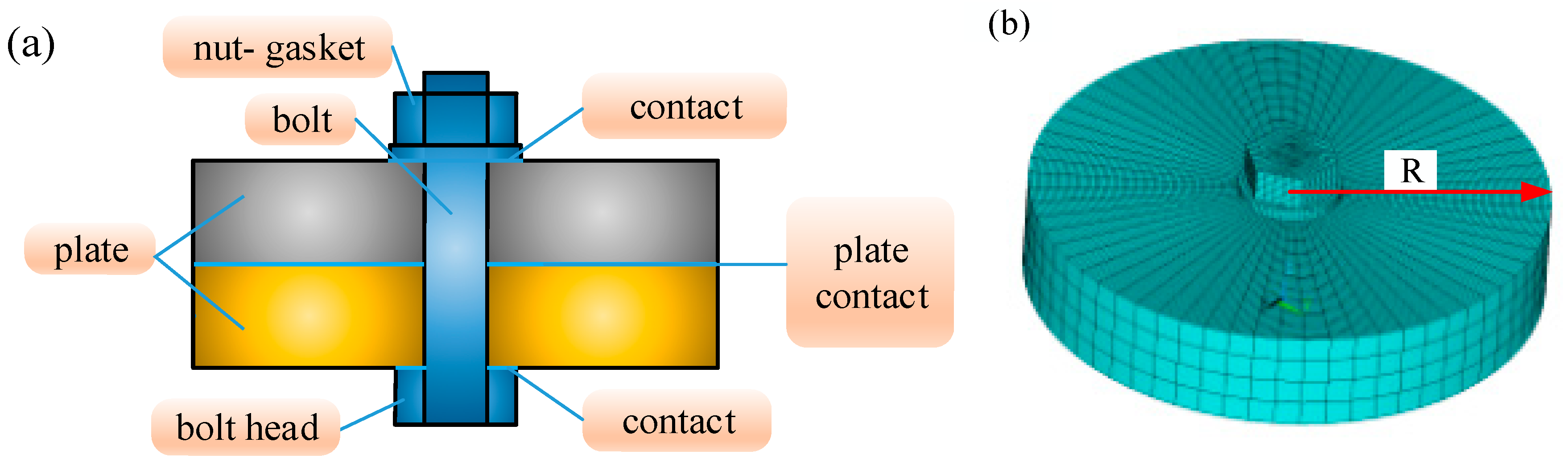
Furthermore, the size of contact area is ambiguity. Often the geometric interface, instead of the ‘real’ physical interface, is used for modeling bolt connections. It must be noted that the influence zone of the bolt connections is not infinite but finite. To illustrate the phenomenon of the finite influence zone, a finite element contact analysis, as an example, is used to study the contact characteristics of bolt connection structures. The contact analysis is performed. The finite element model is constructed by two plates connected with a bolt, which is shown in Figure 1a, the contact element are added between the two plates, the gasket plate, and the bolt head-plate. The element meshing of the whole structure is shown in Figure 1b. It should be mentioned that, due to the axial symmetry of contact pressure, the element size along the R-axis is set small to reduce the influence of element size on the results, and the element size in the other direction is somewhat coarse to reduce the computational cost.

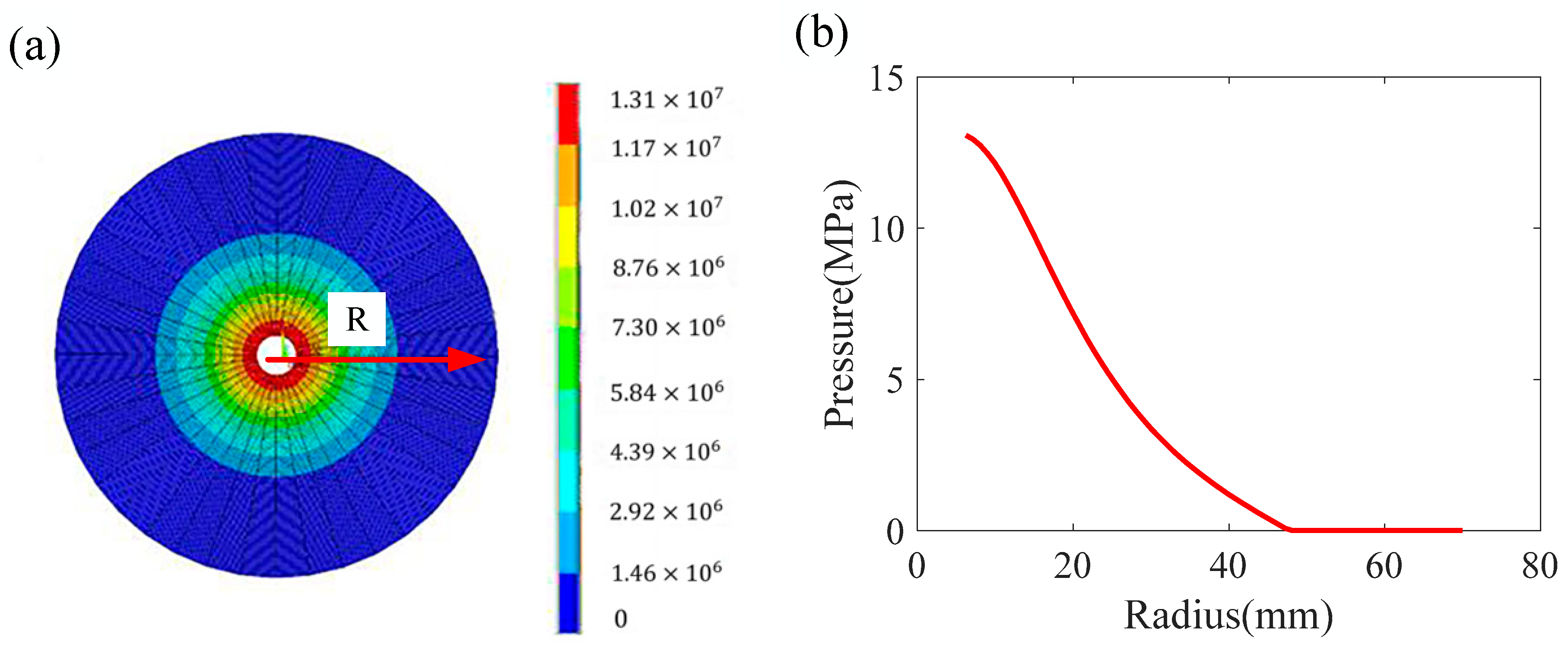
The results of contact analysis can be seen in Figure 2a. As can be seen from the analytical results, the influence of bolted joints on structure exhibits strong local characteristics. To obtain the distribution of the contact pressure between the plates, the values of contact pressure along the R-axis are extracted and drawn in Figure 2b.

It is clear that the influence zone of the bolt connections is finite. For the static connection using bolts, we assume that both the displacement field and the traction satisfy the continuity conditions, which require

$$⟦u_i⟧=0$$

(2)

$$⟦{\sigma }_{ij}{n}_j⟧=0$$

(3)

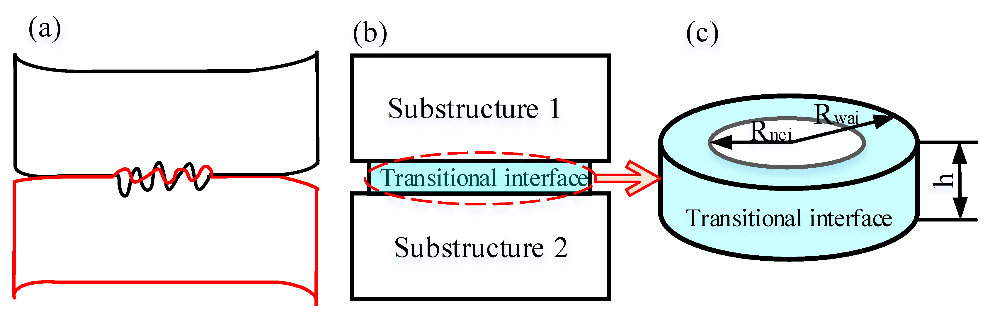
Here, $u_i$ is the displacement field. As defined before, the operator ⟦•⟧ denotes the discrepancy of $•$. These two conditions mean that there is no discrepancy of the upper and lower contacting interface for displacement field and the traction. With these assumptions, we propose the transitional interface model, as shown in Figure 3a. As the bolt-connected structure can be treated as two substructures bolted together under the action of preloads, the ‘real’ physical contact area is a key factor that affects the connection performance. That is, the essence of bolt connection can be alternatively viewed as a local (finite) interface problem. Regarding this, the joint is modeled as a piece of the transition interface material with geometric parameters shown in Figure 3b. The geometric parameters of the transition interface material reflect the actual contact area and the thickness of the transition interface material. The geometric parameters can be calibrated based on experimental data.

As the connecting area of the bolt joint usually acts as circles, the geometric parameters of the virtual material can be modeled as a concentric ring with a certain thickness h, which is shown in Figure 3c. The inner diameter of the concentric ring $R_{nei}$ is related to the diameter of the bolt hole. According to the contact analysis results, the actual contact area of the concentric ring is related to the thickness of the connecting plate and the bolt tightening force. So, the outside diameter of the concentric ring $R_{wai}$, which is related to the thickness b of the connected substructure and the tightening force F of the bolt, is defined as Equation (5). The thickness of the concentric ring h is related to the material properties and surface roughness of the connected substructure, as well as the normal load, which can be defined as

$$R_{nei}=R_{nei}(D)$$

(4)

$$R_{wai}=R_{wai}(b,F)$$

(5)

$$h=h(E_1,E_2,{\mu }_1,{\mu }_2,R_{a1},R_{a2},P)$$

(6)

Here, D means the diameter of the bolt hole, b means the thickness of the connected substructure, F means the tightening force of the bolt, and E₁ and E₂ mean the elastic modulus of the connected substructure, respectively. ${\mu }_1$ and ${\mu }_2$ mean the Poisson’s ratio of the connected substructures. $R_{a1}$ and $R_{a2}$ mean the surface roughness of the connected substructures. $P$ is the normal pressure between the bolt joint and the connected substructure.

As mentioned above, the transition interface material is an interface problem, thus the physical or material properties shall be different to those of its connecting bodies. To explore the feature of the transition interface material, we use the control variable method to clarify the affection of different contact conditions. To illustrate the affection of thickness, the bolt diameter and the tightening force are set as M12 and 25,000 N, respectively. The contact pressure under the thickness value of 10 mm, 20 mm, 30 mm, and 40 mm is analyzed. The contact pressure distribution between the plates modeled using different thicknesses is shown in Figure 4. Clearly, the physical properties of the transition interface material shall change smoothly through its thickness as a gradient way.

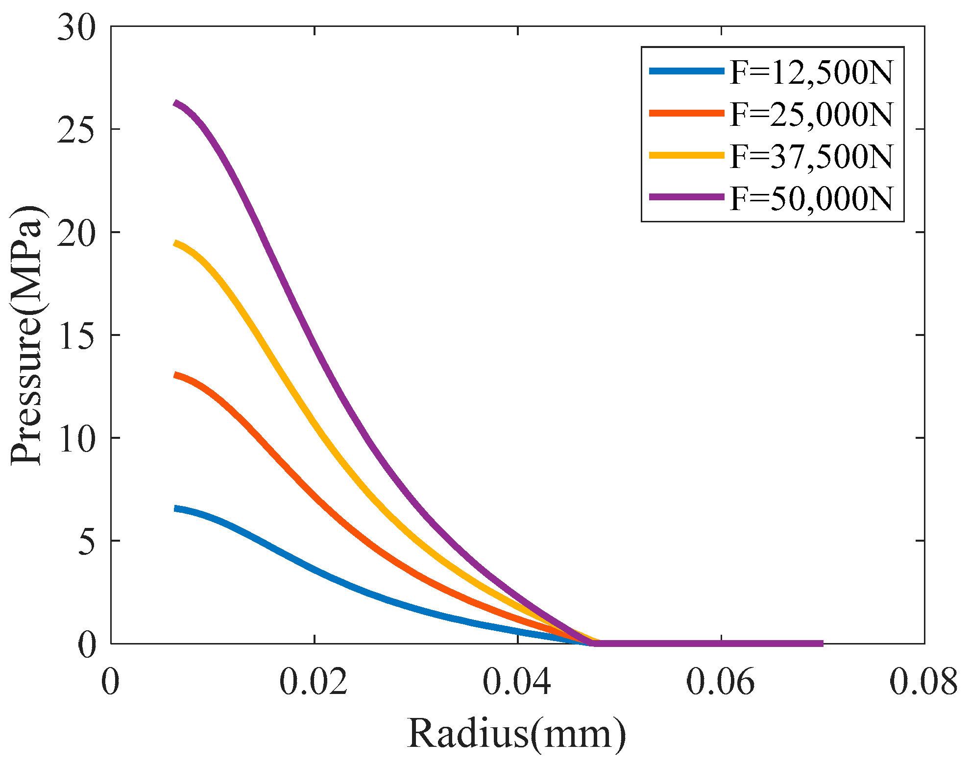
To clarify the affection of tightening force, the bolt diameter and thickness are constant, and the contact pressure distribution between the plates under different tightening forces is drawn in Figure 5. The same process is performed to clarify the affection of bolt diameter, material, and roughness. The result shows that the affection of bolt diameter on the contact pressure distribution of joint bolt connection structures is not significant.

However, modeling the transition interface material using gradient properties is difficult to implement for engineering applications (using common finite element software). For the sake of simplification, the physical properties of the transition interface material are assumed to be uniform. This simplification is mainly aiming at significantly cutting down the complexity of the problem of concern while retaining its most important features. For these reasons, we assume that the transition interface material is isotropic and its property is uniform (only two independent parameters, that is, the elastic modulus $E$ and the Poisson’s ratio $\mu$).

The physical parameters of the transition interface model are reflected mechanical properties of the contact area, which describe the contact stiffness of the surface. Those parameters are mainly determined by the contact pressure. As the contact pressure is related to normal pressure between the joint, the material of contact structure, and the surface roughness. So, the physical parameters of the transition interface material can be defined as

$$E=E(E_1,E_2,{\mu }_1,{\mu }_2,R_{a1},R_{a2},P)$$

(7)

$$\mu =\mu (E_1,E_2,{\mu }_1,{\mu }_2,R_{a1},R_{a2},P)$$

(8)

$$\rho =\rho (E_1,E_2,{\mu }_1,{\mu }_2,R_{a1},R_{a2},P)$$

(9)

Additionally, the density expressed in Equation (9) can be set to zero. This is because the density of the connecting bodies is assumed to unchanged.

The geometric parameters of the transition interface reflect the actual contact area and the thickness of the transition interface material. The physical parameters of the transition interface material reflect the mechanical properties caused by the contact pressure of the contact area. The transition interface material is fixedly connected with the substructure in the contact surface and the material properties changes at the connection part. The connected bolt structure and the transition interface model are shown in Figure 3a,b, respectively.

The sizes of the contact area and the contact pressure on this area are the main factors affecting the connection performance. Clarifying the affection of contact conditions (material, thickness, bolt diameter, tightening force, and so on) on the contact characteristics is the basis of joint modeling.

The transition interface model of the bolt joint proposed in this part has geometric parameters and physical parameters. The geometric parameters describe the geometric dimensions of the actual contact area of the joint, and the physical parameters describe the mechanical properties of the contact area. The application of this model can be shown in Figure 6 According to the surface condition parameters, the geometric and physical parameters of the combined surface are determined. After that, the model is meshed according to the geometric parameters and the physical parameters are given to the mesh. Then, the finite element model of the joint is developed.

As can be seen from Figure 6, the transition interface model takes full consideration of the actual contact situation of the joint in the modeling so that this model is universal. The transition interface model consists of geometric parameters and physical parameters, which can be easily connected with the general finite element software. Moreover, the mesh size of the joint can be conveniently controlled to meet the analysis requirements of different precision.

The application of the proposed transition interface model requires the determination of geometric parameters and physical parameters. As $R_{nei}$ can be given by the connection condition of bolt diameter, the density of virtual can be determined by the average density of the contact plates. The parameters which need to be determined are the geometric parameters R_wai and h, as well as the physical parameters E and $\mu$. The next two sections introduce the parameter identification of transition interface model mode. The contact analysis is conducted to determine the geometric parameters and the average normal pressures of the contact area. After that, the physical parameters are identified by the model updating method because the joint significantly affects the dynamic characteristics of the whole structure.

3. Geometric Parameters Identification of the Transition Interface Model

3.1. Identification of Geometric Parameter R_wai

As can be seen from Figure 2, the pressure distribution is closely related to the radius R. To obtain the real contact area and contact pressure of the bolt joint, the contact pressure between the plant can be extracted. The contact pressure distribution along the radius R can be then drawn by MATLAB. The real contact area can be then obtained by setting a limit for contact pressure such as the contact pressure being larger than P_lim. The expression of the progress can be given as follows:

$$R_{wai}=\max \left\{r|P(r)\ge P_{lim}\right\}$$

(10)

The geometric parameter $R_{wai}$ can be calculated by Equation (10). It should be noted that the element size along the radius R is set very small to ensure the accuracy of the calculation result. By setting the P_lim to 1 MPa, the contact pressure of bolt connect plates with the thickness of 20 mm under different tightening forces can be solved, as shown in

Table 1. The contact radius under different tightening force.

Tightening force (N)	12,500	25,000	37,500	50,000	62,500
Contact radius (mm)	35.39	40.86	42.68	43.59	45.41

.

3.2. Database of the Geometric Parameter of Bolt Joint on Machine Tools

As the plate thickness and the tightening force are the key factors which deeply affect the contact area of bolt connect structure, a database of geometric parameter R_wai of bolt joint on machine tools can be established under the thought of the response surface method. According to the common application of bolt joints on machine tools, the thickness between 10~40 mm and the bolt tightening force between 10,000 N~70,000 N are usually used. This connect condition can be used as samples to form the geometric parameters database. The contact analysis of all combinations under different thicknesses and different tightening forces is performed, and then the real contact radius of the bolt joint and the average contact pressure can be calculated. The results of contact radius and contact pressure are shown in

Table 2. The contact radius under different connection conditions (mm).

	Thickness	10 mm	15 mm	20 mm	25 mm	30 mm	35 mm	40 mm
Tightening Force
12,500 N		25.63	31.54	35.39	36.8	37.86	38.39	39.19
25,000 N		26.25	34.69	40.86	46.29	49.45	50.5	51.79
37,500 N		26.88	35.75	42.68	49.45	54.71	56.82	57.14
50,000 N		27.5	36.8	43.59	51.55	57.88	59.98	61.16
62,500 N		28.36	39.96	45.41	52.61	59.98	63.14	63.84

and

Table 3. The contact pressure under different connection conditions (Mpa).

	Thickness	10 mm	15 mm	20 mm	25 mm	30 mm	35 mm	40 mm
Tightening Force
12,500 N		6.32	3.87	2.87	2.26	1.94	1.82	1.70
25,000 N		11.57	6.61	4.65	3.49	2.87	2.68	2.49
37,500 N		16.77	9.49	6.47	4.72	3.73	3.44	3.29
50,000 N		22.05	11.83	8.35	5.89	4.58	4.21	3.99
62,500 N		27.03	12.15	9.64	7.11	5.42	4.82	4.67

, respectively.

After determining the contact radius at the sample points, the interpolation method can be conducted to estimate the contact radius under the actual application. The Kriging interpolation method, which is a local interpolation method based on variogram theory, is chosen as the interpolation method for contact radius estimation. This method assumed that the response value consists of a regression model $g(t)$ and random process function $Z(t)$

$$\widehat{f}(t)=g(t)+Z(t)$$

(11)

The regression model $g(t)$ is selected according to the characteristics of the measured data. The random process function $Z(t)$ has the mean equal to zero and the non-zero covariance. The value of the function at the point $t_0$ which needs to be estimated can be expressed as

$$z(t_0)={\displaystyle \sum _{i=1}^n{\lambda }_{i}z(t_i)}$$

(12)

Here, $t_i(i=1,2,\dots ,n)$ represents known sample points, and $z(t_i)$ represents the value of known sample points; ${\lambda }_i$ is the undetermined weight coefficient which can be obtained by joint solution according to the unbiased condition and the minimum variance condition:

$$\{\begin{array}{l}{\displaystyle \sum _{i=1}^n{\lambda }_{i}C(t_i,t_j)-\mu =\overline{C}(t_i,V) (i=1,2,\dots ,n)}\\ {\displaystyle \sum _{i=1}^n{\lambda }_i}=1\end{array}$$

(13)

Based on the effect radius in Table 2, The Kriging interpolation method can be conducted for the estimation of $R_{wai}$. To check the accuracy of the Kriging interpolation method, the total 35 data points in Table 2 are classified as the sample points set and the testing points set. The sample points are used to form the Kriging method and the testing points are used for comparison. The testing points set are chosen in

Table 4. The contact radius of testing points.

Testing Point	Tightening Force (N)	Thickness (mm)	Analyzed Contact Radius (mm)
1	12,500	30	37.86
2	25,000	15	34.69
3	37,500	25	49.45
4	50,000	20	43.59
5	62,500	35	63.14

, and the others in Table 2 are used as sample points.

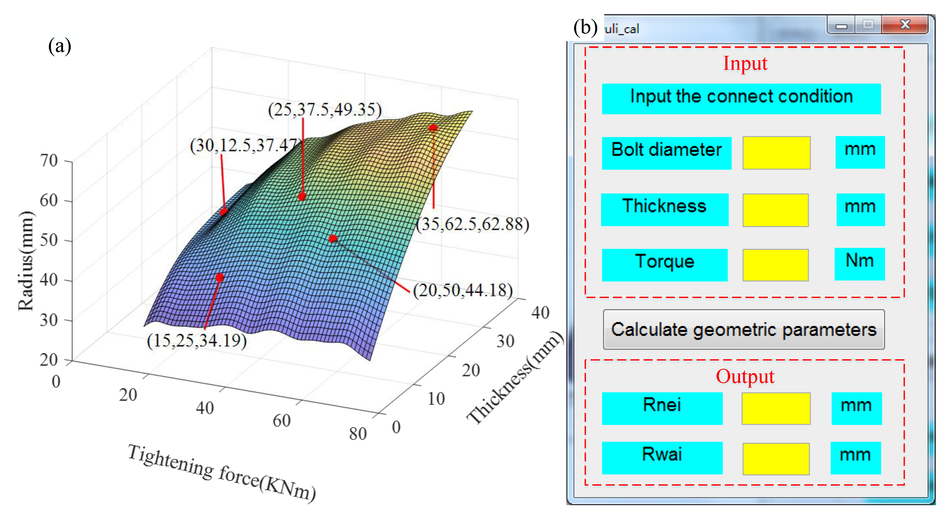
The Kriging interpolation of contact radius under different connect thicknesses and tightening forces is shown in Figure 7a.

The contact radius estimated by the Kriging interpolation method under the testing points is shown in

Table 5. The error of contact radius estimated by the Kriging interpolation method.

Testing Point	Analyzed Contact Radius (mm)	Estimated Contact Radius (mm)	Errors (%)
1	37.86	37.47	−1.03
2	34.69	34.19	−1.44
3	49.45	49.34	−0.22
4	43.59	44.18	1.35
5	63.14	62.88	−0.41

and the errors are listed in the last column of the table. As can be seen from the results, the contact radius estimated by the Kriging interpolation method is less than 2%, which means that the constructed geometric parameter database can be used for engineering applications.

To make the database more usable, a parameter database management system is developed by MATLAB GUI as Figure 7b. It should be mentioned here that as the tightening torque and bolt diameter is usually used in engineering applications, the parameter database management system uses the tightening torque and bolt diameter as input, the tightening force is calculated from the inputs and the Kriging interpolation method is then used to calculate the contact radius.

The average contact pressure P, which is used as the input of physical parameters identification, can also be calculated by the same progress under the Kriging interpolation method.

4. Physical Parameters Identification of the Transition Interface Model

Once the geometric parameter R_wai of the proposed model is identified, the unknown parameters of the proposed model are the physical parameters and thickness. In this section, the parameter identification method for those unknown parameters is introduced firstly. Then, the accuracy of the proposed parameter identification method is verified through numerical example. After that, the joint parameters are identified and the accuracy of the proposed joint model is verified

4.1. Physical Parameters Identification Based on Model Updating Method

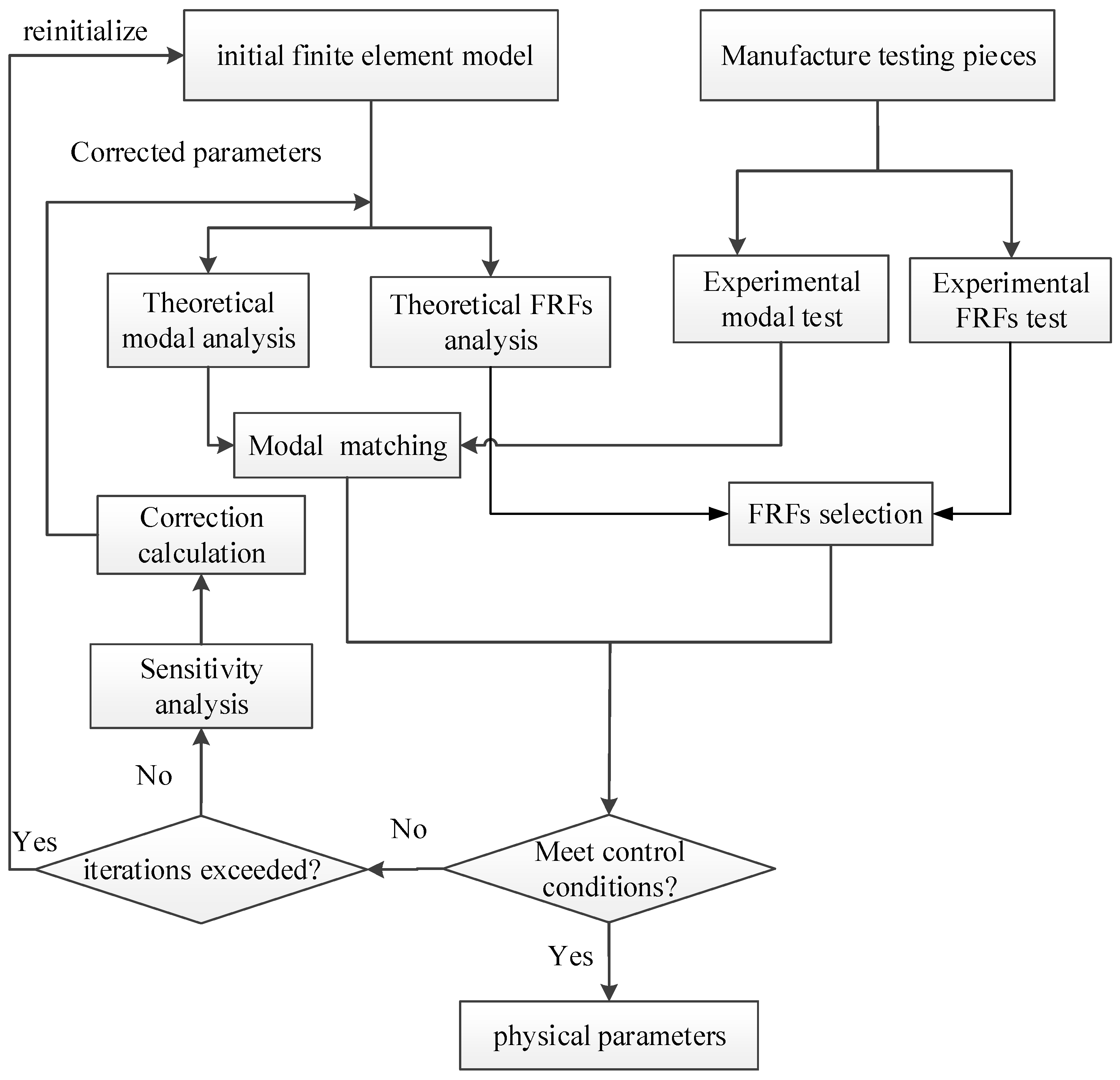
According to the transition interface model, the bolt connects structure can be treated as substructures of plates and substructures of the bolt joint. The dynamic characteristics of the whole structure and the substructures of plates are known. The model updating method can be performed to identify the bolt joint. Due to the limitation of testing condition, the number of test modal is usually limited which make the parameter identification method based on modal parameters easy to face statically indeterminate problems. The frequency response function contains much dynamic information about the structure; however, the parameter identification method based on FRFs has to treat the inverse problem, which is very sensitive to measuring noise. A new method that combines the modal parameters and FRFs by weight matrix is proposed to overcome the shortcomings of both methods. The FRFs are properly introduced to the model updating equations base on modal parameters. Those equations are weighting properties to reduce the conditions which could improve the precision and stability of parameter identification. The process of parameter identification is shown in Figure 8.

Choosing the natural frequency and FRFs as the objective function, the identification control conditions can be set as Equation (7),

$$\{\begin{array}{c}\left|\frac{w_i^{ana}(\mathsf{\Delta }p)-w_i^{ex}}{w_i^{ex}}\right|\le {\epsilon }_1 \mathrm{for} i=1,2,\dots ,n\\ \left|\frac{H_{j,kt}^{ana}(\mathsf{\Delta }p)-H_{j,kt}^{ex}}{H_{j,kt}^{ex}}\right|\le {\epsilon }_2 \mathrm{for} j=1,2,\dots ,N\end{array}$$

(14)

Here, $w_i^{ana}$ and $w_i^{ex}$ are ith order theoretical and experimental natural frequency, respectively. $H_{j,kt}^{ana}$ and $H_{j,kt}^{ex}$ are the theoretical and experimental FRFs which excited at t degrees of freedom and response on k degrees of freedom, respectively. Variables n and N are the numbers of mode and FRFs which take part in the parameter identification, respectively. ${\epsilon }_1$ and ${\epsilon }_2$ are the tolerance of natural frequency and FRFs, respectively. $\mathsf{\Delta }p$ are the parameters which need to be modified, which can be the elastic modulus, Poisson’s ratio, the thickness et al.

For the joint parameter identification problem with m unknown variables, the modified equations can be constructed by the first few natural frequencies and some chosen FRFs, and the equation is formed as follows:

$$A{x}_p=b$$

(15)

where

$$A=\left\{\begin{array}{c}{A}_1\\ A_2\end{array}\right\},A_1=\left[\begin{array}{ccc}\frac{\partial w_1}{\partial p_1}& \dots & \frac{\partial w_1}{\partial p_m}\\ \dots & \dots & \dots \\ \frac{\partial w_n}{\partial p_1}& \dots & \frac{\partial w_n}{\partial p_m}\end{array}\right],A_2=\left[\begin{array}{ccc}\frac{\partial H_{1,kt}}{\partial p_1}& \dots & \frac{\partial H_{1,kt}}{\partial p_m}\\ \dots & \dots & \dots \\ \frac{\partial H_{N,kt}}{\partial p_1}& \dots & \frac{\partial H_{N,kt}}{\partial p_m}\end{array}\right]$$

(16)

$$b=\left\{\begin{array}{c}{b}_1\\ b_2\end{array}\right\},b_1=\left[\begin{array}{c}{w}_1^{ex}-w_1^{ana}\\ \dots \\ w_n^{ex}-w_n^{ana}\end{array}\right],b_2=\left[\begin{array}{c}{H}_{1,kt}^{ex}-H_{1,kt}^{ana}\\ \dots \\ H_{N,kt}^{ex}-H_{N,kt}^{ana}\end{array}\right],x_p=\left[\begin{array}{c}{x}_{p1}\\ \dots \\ x_{pm}\end{array}\right]$$

(17)

Once the sensitivity of natural frequencies and FRFs are calculated, the modified parameters $x_p$ can be calculated by Equation (15). For the transition interface model constructed in this study, the modified parameters are defined as $x_p={[\begin{array}{ccc}E& \mu & h\end{array}]}^T$. The joint parameters can then be identified as the iteration progress shown in Figure 4.

As the sensitivity values of natural frequency to different parameters ($E$, $\mu$ and $h$) varied greatly, the modified Equation (15) usually faces an ill-condition problem, which makes the modified progress disconverge. The treatment of this problem is the key to the parameter identification progress. A new weighted equation shown as Equation (18) is proposed to reduce the condition number of the modified equation,

$$W_{m}A{W}_p{x}_{wp}=W_{m}b$$

(18)

Here,

$$W_m=diag\left(\left\{\underset{n}{\underbrace{\begin{array}{ccc}\frac{w_{f_1}}{{\displaystyle \sum _{i=1}^m\left|A_{f_1,p_i}\right|}}& \cdots & \frac{w_{f_n}}{{\displaystyle \sum _{i=1}^m\left|A_{f_n,p_i}\right|}}\end{array}}}\right\},\left\{\underset{N}{\underbrace{\begin{array}{ccc}\frac{w_{H_1}}{{\displaystyle \sum _{i=1}^m\left|A_{H_{1,kt},p_i}\right|}}& \cdots & \frac{w_{H_n}}{{\displaystyle \sum _{i=1}^m\left|A_{H_{N,kt},p_i}\right|}}\end{array}}}\right\}\right)$$

(19)

$$W_p=diag\left(\underset{m}{\underbrace{\frac{1}{{\displaystyle \sum _{i=1}^n\left|A_{f,p_1}^i\right|+{\displaystyle \sum _{j=1}^N\left|A_{H_{j,kt},p_1}\right|}}},\frac{1}{{\displaystyle \sum _{i=1}^n\left|A_{f,p_2}^i\right|+{\displaystyle \sum _{i=1}^N\left|A_{H_{j,kt},p_2}\right|}}},\dots ,\frac{1}{{\displaystyle \sum _{i=1}^n\left|A_{f,p_m}^i\right|+{\displaystyle \sum _{i=1}^N\left|A_{H_{j,kt},p_m}\right|}}}}}\right)$$

(20)

Here, the left weight function $W_m$ is the inverse of the sum of absolute values to the sensitivities of all design parameters, which aim to reduce the difference in sensitivity values between certain identification parameters to the different modal parameters. The right weight function $W_p$ is the inverse of the sum of the absolute value of the sensitivity of design parameters to all modal parameters and all FRFs, which aims to reduce the difference of sensitivity values between different identification parameters to certain modal parameters.

4.2. Validation of the Physical Parameter Identification Method

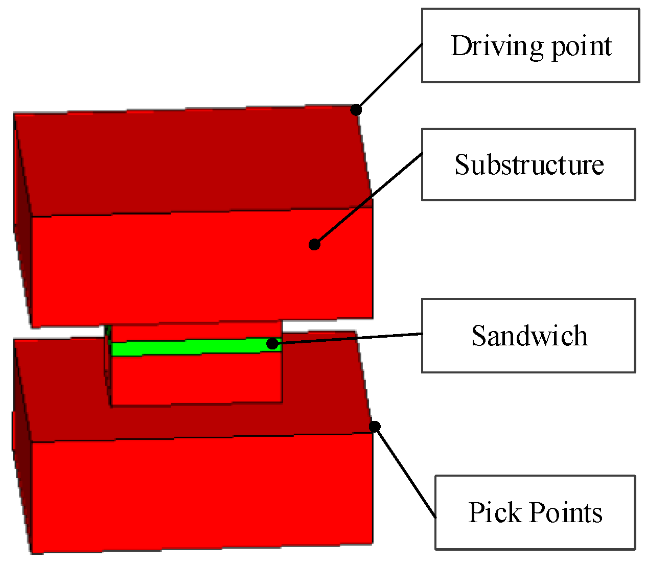
To verify the accuracy of the physical parameter identification method proposed in Section 4.1, the theoretical model of two dumbbells connected by a sandwich material, as shown in Figure 9, is constructed. The elastic modulus and Poisson’s ratio of dumbbells are 1.3 × 10¹¹ Pa and 0.27, respectively. The density of the model is 7850 kg/m³. The thickness and the elastic modulus as well as the Poisson’s ratio of the sandwich are the unknown parameters that need to be identified. The pickup and driving points of the FRFs in the theoretical model are shown in Figure 9.

The sandwich material under material parameters 1 in

Table 6. Material parameters of sandwich.

	Thickness h (mm)	Elastic Modulus Ej (Pa)	$\mathbf{Poisson} \mathbf{Ratio} \mathit{\mu }$
Material parameters 1	10	1 × 1010	0.24
Material parameters 2	20	3.5 × 1010	0.27

is chosen as the standard structure. The model analysis is performed to this standard structure to obtain the non-zero natural frequencies and modals. Additionally, the frequency response function analysis is performed to obtain the FRFs. Those analysis results are treated as the experimental results.

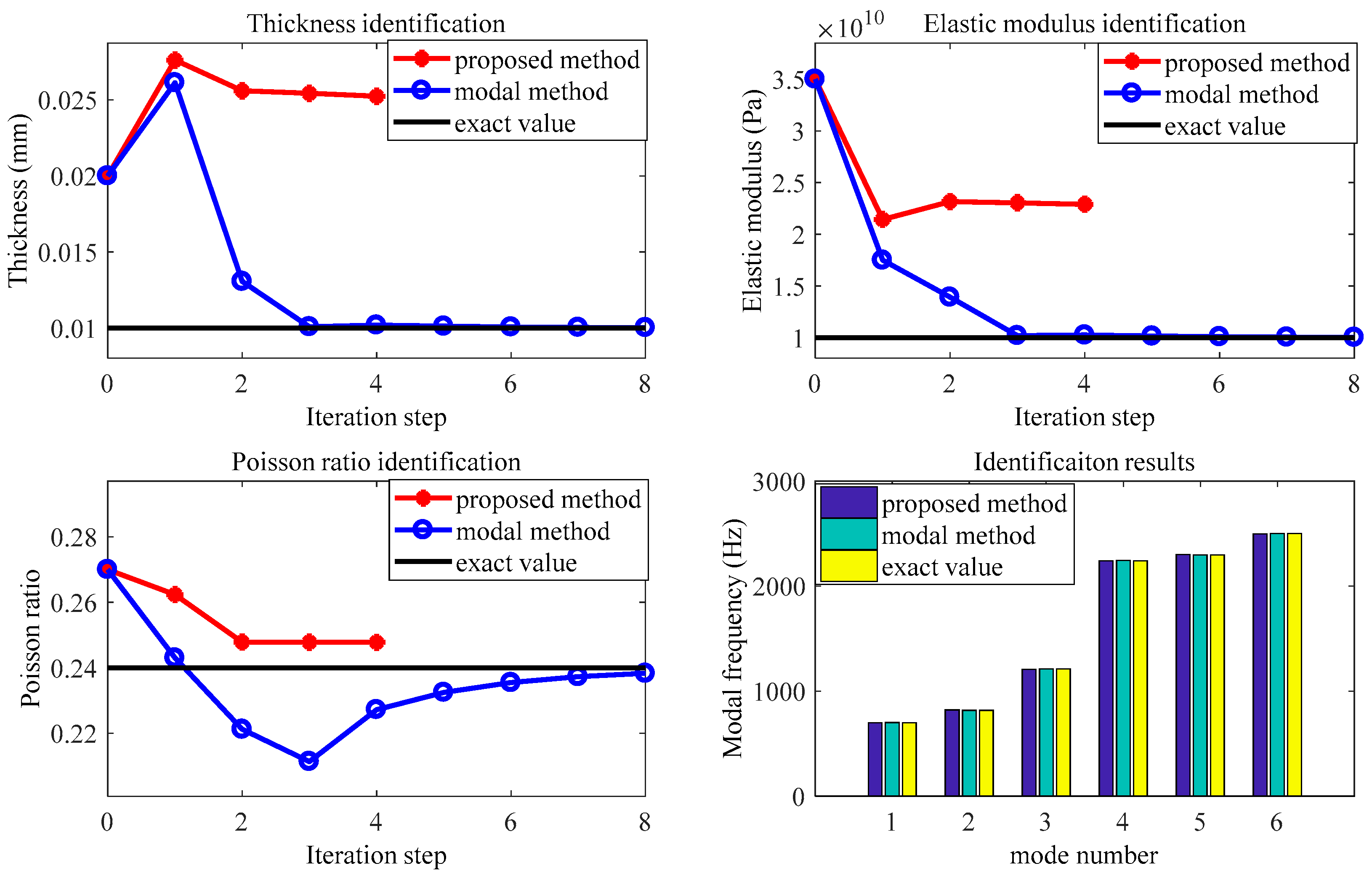
The sandwich material under material parameter 2 is set as the initial parameters. The method proposed in Section 4.1 is adopted for parameter identification. For the aim of comparison, the model-based method which used the first six order modal data for parameter identification is also produced. The iterative process and correction results of the two methods are shown in Figure 10.

As can be seen from Figure 10, the proposed method could identify the parameters of the sandwich with high accuracy. Although the model-based method could make the natural frequencies of the modified system have good agreement with the experimental results after a few steps of iterations, it failed to identify the exact result of the sandwich parameters. The reason is that just a few experiment modes may not be enough to describe all the characteristics of the system. The result of parameter identification may not be unique when just a few modes are used in the identification process. The method proposed in Section 4.1 uses FRFs as a supplement to the identification process, which could describe the system more accurately and improve the accuracy of parameter identification.

4.3. Validation of the Dynamic Model of Bolt Joint

To check the effectiveness of the dynamic model proposed in this paper, experimental specimens were designed and manufactured, and the joint parameters were identified by the parameter identification method proposed in Section 4.1.

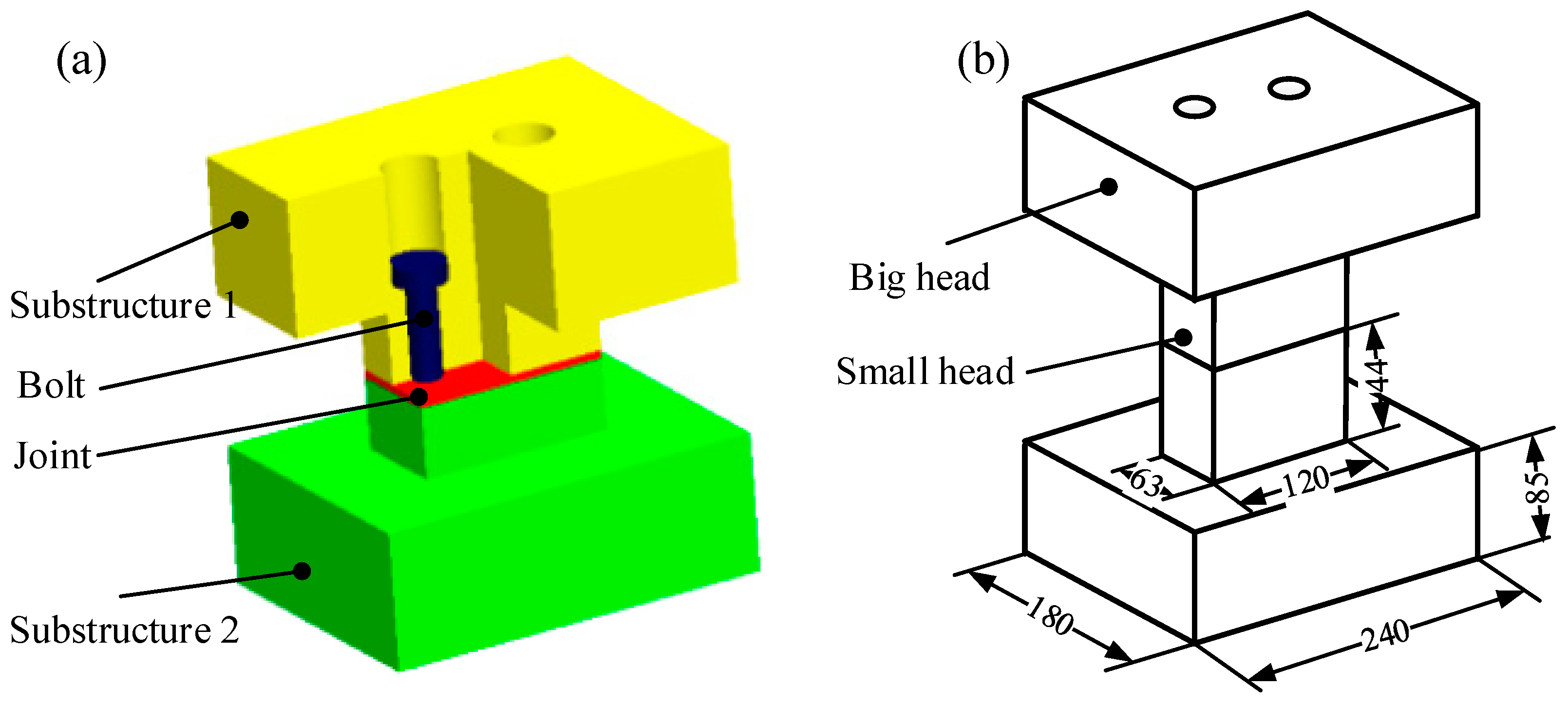
As shown in Figure 11, the dumbbell-like experimental specimen which has a small head near the contact part of the bolt joint is manufactured. This design would make the joint-related part ‘soft’ so that the dynamic characteristics of the bolt connection part could be inspired easily. The length and width of the big bead and the small bead of the dumbbell-like experimental specimen are 240 × 180 mm and 120 × 63 mm, respectively. The roughness of the surface is $Ra=1.6 \mathsf{\mu }\mathrm{m}$, the diameter of the bolt is M16, and the preload of the bolt in the experiment is 90 Nm.

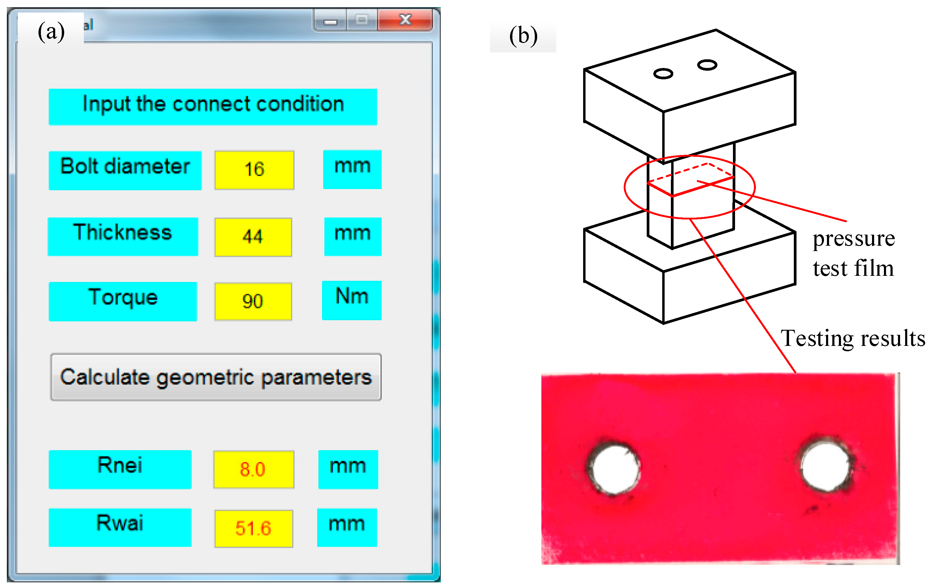
By inputting the contact conditions to the geometric parameter database constructed in Section 3.2, the contact radius of the experimental specimen can be calculated as Figure 12. By comparing the dimension of the small head with the contact radius R_wai seen in Figure 12a, it can be obtained that the contact occurs on the whole surface. To illustrate this result, the contact pressure test film which consists of two pieces of thin film produced by the Fuji company is used for contact pressure testing. The film is inserted into the contact area, and the colors change to red once the contact pressure is large than 1 Mpa. The pressure testing is shown in Figure 12b, and the results demonstrated that the contact fulfills the whole surface. The geometric model of the bolt joint can then be established.

The impact experimental test system includes the LMS Test.Lab 9B vibration Test and analysis system, PCB086D05 hammer, and PCB356A15 acceleration sensors. The test pieces are suspended by wire rope as shown in Figure 13a to simulate the free boundary. To reduce the influence of additional quality of sensors on test results, only one sensor is attached at a time during the test. As shown in Figure 13b, the whole system is arranged as a total of 72 measuring points. The x and z directions of point 57 are taken as the excitation directions in the experiment.

The Time MDOF modal analysis method is used to obtain the modal frequency and modal shapes of the specimen. After that, the method proposed in Section 4.1 is carried out, and the experimental modal frequency and modal shape, as well as the FRFs, are used for physical parameter identification. As the contact radius is determined, only the thickness and elastic modulus, as well as the Poisson’s ratio of the joint, are needed to be identified. The identification progress is implemented by the MATLAB program and the material parameters of the joint are obtained after repeated iterative solutions. The results are shown in

Table 7. Parameters identification results.

Parameters	Thickness h (mm)	Elastic Modulus Ej (MPa)	Poisson Ratio ($\mathit{\mu }$)
Value	0.657	1513	0.201

.

Once the joint parameters are identified, the theoretical model of the whole system which contained the joints and the sub-dumbbell-like structures can be constructed. The theoretical modal parameters can then be obtained by finite element analysis. The validation of the proposed joint model can be verified by comparing the theoretical modal parameters with the experimental results. The modal shapes of both methods are shown in

Table 8. Comparison of the theoretical modes and experimental modes.

Model	Spin Z-Axis	Spin X-Axis	Spin Y-Axis
Experimental model
theoretical modal
MAC	0.969	0.908	0.903
Model	Translation Y-Axis	Translation X-Axis	Translation Z-Axis
Experimental model
Theoretical modal
MAC	0.741	0.785	0.855

.

As can be seen from Table 8, the MAC value of the first three modes are greater than 90%, and that of all the first six modes are bigger than 0.74, which means that the first six modes are matched one by one. Based on this, the modal frequencies of the first sixth modes are compared in

Table 9. Comparison of the theoretical modal frequency and experimental modal frequency (Hz).

	Spin Z-Axis	Spin X-Axis	Spin Y-Axis	Translation Y-Axis	Translation X-Axis	Translation Z-Axis
Experimental frequency	846.9	1026.3	1386.3	2428.7	2626.7	2762
Theoretical frequency	801.22	949.67	1386.5	2501.3	2547.1	2786.8
Errors (%)	5.39	7.47	−0.02	−2.99	3.08	−0.9

.

As can be seen from the results in Table 9, the modal frequency errors of all the six models are less than 7.5%, while for the eight-nodes-hexahedron-element model proposed in Ref. [9], the frequency errors are up to 15.7%. This is because that the eight-nodes-hexahedron-element model just considered the coupling relation between the edge nodes of the joint, and the coupling relationships within the inner contact surface are ignored. As for the virtual material model proposed by Tian [14], once the material parameter are calculated by Hertz contact theory and fractal theory, the frequency errors of dumbbell-like structure in ref are within 10%, which is larger than the proposed transition interface model. Those comparison results demonstrated that the proposed transition interface model is accurate for joint modeling.

Based on the proposed transition interface model and the parameter identification method, a database of bolt joints can be established by the consideration of the diameter of the bolt, thickness, tightening force, and surface roughness. Additionally, this database can be used for structural analysis and structural optimization design.

5. Application of the Transition Interface Model to Machine Tools

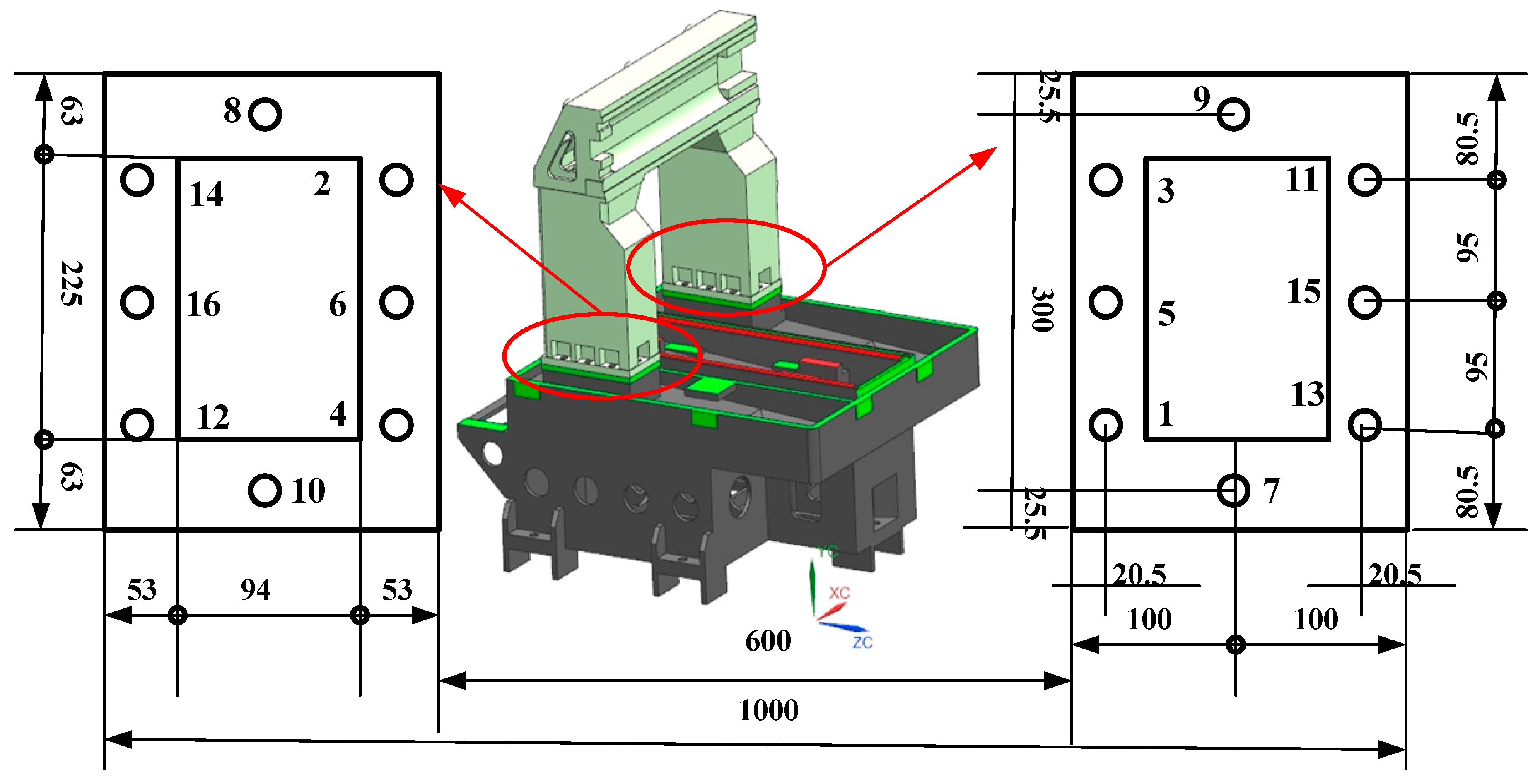
In this section, an engraving machine tool is used as an example to illustrate the engineering application of the proposed transition interface model. The major part of the engraving machine is the bed and the column which are connected by 16 bolts. The frame and the bolts distribution are shown in Figure 14.

The connect condition of the bolts is listed in

Table 10. Connect condition of the bolts.

Bolt Number	Bolt Diameter	Tightening Torque	Surface Roughness	Thickness
1–16	M12	120 Nm	1.6 μm	25 mm

.

The connecting area of the bolt can be calculated from the database constructed in Section 3.2. The Young’s modulus and the Poisson’s ratio of the bed and the colon are E = 1.5 × 10¹¹ Nm and μ = 0.23. Additionally, the physical parameters of the transition interface model are calculated to form the physical parameter database and are shown in

Table 11. Parameters of the transition interface model.

Parameters	Thickness h	Elastic Modulus Ej	$\mathbf{Poisson}’\mathbf{s} \mathbf{Ratio} \mathit{\mu }$
Value	0.72 mm	6111 MPa	0.253

.

The whole meshing of the structure is shown in Figure 15a, the bolt joint-related part is shown as the partial enlarged part and the virtual material of the bolt joint is marked as red color. The whole system is modeled as 73,925 3D elements with 348,111 DOFs, and the free boundary condition is applied in the modal analysis. To construct the free boundary condition, the real system, s as in Figure 15b, is hung for the impact modal experiment.

The first five models are shown in

Table 12. Result of the theoretical analysis and modal experiment.

	Frequency Comparison		Experimental Model Shape	Analysis Model Shape
First model	Experimental result (Hz)	145.81
	Theoretical result (Hz)	147.14
	Error	−0.91%
Second model	Experimental result (Hz)	155.07
	Theoretical result (Hz)	155.05
	Error	0.01%
Third model	Experimental result (Hz)	216.61
	Theoretical result (Hz)	218.68
	Error	−0.96%
Forth model	Experimental result (Hz)	244.13
	Theoretical result (Hz)	237.39
	Error	2.76%
Fifth model	Experimental result (Hz)	441.46
	Theoretical result (Hz)	439.65
	Error	0.41%

. The difference between the first five modal frequencies between the theoretical model modal and the experimental results are less than 3%, which means that the proposed transition interface model and constructed database have high accuracy. Additionally, it can be used for engineering applications such as structural optimization design and structural health monitoring.

6. Conclusions

This paper aimed at the dynamic modeling and parameter identification of bolt joints. The main work can be concluded as follows:

(1) Based on the fact that the characteristics of bolt joints rely on the contact area and contact pressure of the surface, and assuming there is no discrepancy of the upper and lower contacting interfaces for displacement field and the traction, a transition interface model of bolt joints containing geometric and physical parameters is proposed.

(2) The contact radius of the bolt joint is calculated based on the contact analysis, and the geometric parameter database of bolt joint on machine tools is established by the Kriging interpolation method. The error of contact radius estimated by the testing point is less than 2%, which verified the accuracy of the established geometric parameter database.

(3) The model updating method, which is constructed by the combination of modal parameters and FRFs, is proposed for physical parameter identification of the transition interface model. Additionally, a numerical example is used to check the validity of the proposed identification method. The results show that once the FRFs are added and weighted with the left and right weight matrix to the identification process, the proposed method is accurate for parameter identification of the transition interface model.

(4) A dumbbell-like experimental system containing the bolt joints is designed and manufactured for joint parameter identification and joint model validation. The difference in the first six order modal frequencies between the theoretical model analysis and the experimental results is less than 7.5%, which means that the proposed joint model is accurate.

(5) The frame of the engraving machine tool is used to check the effectiveness of the proposed transition interface model and the good agreement of the analysis modal frequency, and the experimental results demonstrated that the proposed model can be used for engineering applications such as structural optimization design and structural health monitoring.

References

- Wang, L.; Liu, H.; Yang, L.; Zhang, J.; Zhao, W.; Lu, B. The effect of axis coupling on machine tool dynamics determined by tool deviation. Int. J. Mach. Tools Manuf. 2015, 88, 71–81. [Google Scholar] [CrossRef]
- Liu, X.; Sun, W.; Fang, Z. Finite element dynamic modeling for bolted thin plate structure based on complex spring element with non-uniform distribution. J. Vib. Shock 2021, 40, 111–119. [Google Scholar]
- Li, Y.; Hao, Z. A six-parameter Iwan model and its application. Mech. Syst. Signal Process. 2016, 68–69, 354–365. [Google Scholar] [CrossRef]
- Li, C.; Qiao, R.; Tang, Q.; Miao, X. Investigation on the vibration and interface state of a thin-walled cylindrical shell with bolted joints considering its bilinear stiffness. Appl. Acoust. 2021, 172, 107580. [Google Scholar] [CrossRef]
- Hohberg, J.-M. A Joint Element for the Nonlinear Dynamic Analysis of Arch Dams; Birkhäuser: Basel, Switzerland, 1992; Volume 186. [Google Scholar]
- Xiao, W.; Mao, K.; Zhu, M.; Li, B.; Lei, S.; Pan, X. Modelling the spindle–holder taper joint in machine tools: A tapered zero-thickness finite element method. J. Sound Vib. 2014, 333, 5836–5850. [Google Scholar] [CrossRef]
- Bograd, S.; Reuss, P.; Schmidt, A.; Gaul, L.; Mayer, M. Modeling the dynamics of mechanical joints. Mech. Syst. Signal Process. 2011, 25, 2801–2826. [Google Scholar] [CrossRef]
- Mao, K.; Li, B.; Wu, J.; Shao, X. Stiffness influential factors-based dynamic modeling and its parameter identification method of fixed joints in machine tools. Int. J. Mach. Tools Manuf. 2010, 50, 156–164. [Google Scholar] [CrossRef]
- MAO, K.; HUANG, X.; LI, B.; Tian, H. Dynamic and parameterized modeling of fixed joints in machine tools using surface respose method. J. Huzhong Univ. Sci. Technol. Nat. Sci. Ed. 2012, 40, 49–53. [Google Scholar]
- Li, L.; Wang, J.; Pei, X.; Chu, W.; Cai, A. A modified elastic contact stiffness model considering the deformation of bulk substrate. J. Mech. Sci. Technol. 2020, 34, 777–790. [Google Scholar] [CrossRef]
- Ling, L.; Qiangqiang, Y.; Jingjing, W.; Yabin, D.; Xiaohui, S. A continuous and smooth contact stiffness model for mechanical joint surface. J. Mech. Eng. 2021, 57, 117–124. [Google Scholar]
- Ahmadian, H.; Jalali, H.; Mottershead, J.; Friswell, M. Dynamic modelling of spot welds using thin-layer interface theory. In Proceedings of the 10th International Congress on Sound and Vibration (ICSV10), Stockholm, Sweden, 7–10 July 2003. [Google Scholar]
- Ahmadian, H.; Mottershead, J.E.; James, S.; Friswell, M.I.; Reece, C.A. Modelling and updating of large surface-to-surface joints in the AWE-MACE structure. Mech. Syst. Signal Process. 2006, 20, 868–880. [Google Scholar] [CrossRef]
- Tian, H.; Li, B.; Liu, H.; Mao, K.; Peng, F.; Huang, X. A new method of virtual material hypothesis-based dynamic modeling on fixed joint interface in machine tools. Int. J. Mach. Tools Manuf. 2011, 51, 239–249. [Google Scholar] [CrossRef]
- Hui, M.; Mingyue, Y.; Ang, G.; Chenguang, Z. Dynamic Modeling Method of Bolted Joint Interfaces Based on Nonlinear Transversely Isotropic Virtual Material. J. Northeast. Univ. (Nat. Sci.) 2021, 42, 1111–1119. [Google Scholar]
- Mantelli, M.; Milanez, F.H.; Pereira, E.; Fletcher, L. Statistical model for pressure distribution of bolted joints. J. Thermophys. Heat Transf. 2010, 24, 432–437. [Google Scholar] [CrossRef]
- Marshall, M.; Zainal, I.; Lewis, R. Influence of the interfacial pressure distribution on loosening of bolted joints. Strain 2011, 47, 65–78. [Google Scholar] [CrossRef]
- Yang, G.; Hong, J.; Wang, N.; Zhu, L.; Ding, Y.; Yang, Z. Member stiffnesses and interface contact characteristics of bolted joints. In Proceedings of the Assembly and Manufacturing (ISAM), Tampere, Finland, 25–27 May 2011; pp. 1–6. [Google Scholar]
- Stephen, J.T. Condition Monitoring of Bolted Joints; University of Sheffield: Sheffield, UK, 2015. [Google Scholar]
- Dekoninck, C. Deformation properties of metallic contact surfaces of joints under the influence of dynamic tangential loads. Int. J. Mach. Tool Des. Res. 1972, 12, 193–199. [Google Scholar] [CrossRef]
- Eriten, M.; Lee, C.-H.; Polycarpou, A.A. Measurements of tangential stiffness and damping of mechanical joints: Direct versus indirect contact resonance methods. Tribol. Int. 2012, 50, 35–44. [Google Scholar] [CrossRef]
- Johnson, K.L.; Johnson, K.L. Contact Mechanics; Cambridge University Press: Cambridge, UK, 1987. [Google Scholar]
- Liou, J.L.; Lin, J.F. A new method developed for fractal dimension and topothesy varying with the mean separation of two contact surfaces. J. Tribol. 2006, 128, 515–524. [Google Scholar] [CrossRef]
- Liou, J.L.; Lin, J.F. A new microcontact model developed for variable fractal dimension, topothesy, density of asperity, and probability density function of asperity heights. J. Appl. Mech. 2007, 74, 603–613. [Google Scholar] [CrossRef]
- Zhao, Y.; Yang, C.; Cai, L.; Shi, W.; Liu, Z. Surface contact stress-based nonlinear virtual material method for dynamic analysis of bolted joint of machine tool. Precis. Eng. 2016, 43, 230–240. [Google Scholar] [CrossRef]
- Liu, W.; Yang, J.; Xi, N.; Shen, J.; Li, L. A study of normal dynamic parameter models of joint interfaces based on fractal theory. J. Adv. Mech. Des. Syst. Manuf. 2015, 9, JAMDSM0070. [Google Scholar] [CrossRef] [Green Version]
- Yonghui, C.; Xueliang, Z.; Shuhua, W.; Guosheng, L. Fractal Model for Normal Contact Damping of Joint Surface Considering Elastoplastic Phase. Chin. J. Mech. Eng. 2019, 55, 58–68. [Google Scholar] [CrossRef]
- Ye, H.; Yumei, H.; Pengyang, L.; Yan, L. static characteristic analysis of bolt joint under preloads. China Mech. Eng. 2019, 30, 1149–1155. [Google Scholar]
- Tsai, J.-S.; Chou, Y.-F. The identification of dynamic characteristics of a single bolt joint. J. Sound Vib. 1988, 125, 487–502. [Google Scholar] [CrossRef]
- Wang, J.; Liou, C. Identification of parameters of structural joints by use of noise-contaminated FRFs. J. Sound Vib. 1990, 142, 261–277. [Google Scholar] [CrossRef]
- Wang, J.-H.; Liou, C.-S. The use of condition number of a FRF matrix in mechanical parameter identification. In Proceedings of the 14th Biennial Conference on Mechanical Vibration and Noise: Vibrations of Mechanical Systems and the History of Mechanical Design, Albuquerque, NM, USA, 19–22 September 1993; pp. 117–124. [Google Scholar]
- Wang, J.; Chuang, S. Reducing errors in the identification of structural joint parameters using error functions. J. Sound Vib. 2004, 273, 295–316. [Google Scholar] [CrossRef]
- Fox, R.; Kapoor, M. Rates of change of eigenvalues and eigenvectors. AIAA J. 1968, 6, 2426–2429. [Google Scholar] [CrossRef]
- Lee, I.-W.; Kim, D.-O.; Jung, G.-H. Natural frequency and mode shape sensitivities of damped systems: Part I, distinct natural frequencies. J. Sound Vib. 1999, 223, 399–412. [Google Scholar] [CrossRef]
- Li, L.; Hu, Y.; Wang, X. Design sensitivity and Hessian matrix of generalized eigenproblems. Mech. Syst. Signal Process. 2014, 43, 272–294. [Google Scholar] [CrossRef]
- Li, L.; Hu, Y.; Wang, X. A study on design sensitivity analysis for general nonlinear eigenproblems. Mech. Syst. Signal Process. 2013, 34, 88–105. [Google Scholar] [CrossRef]
- Wu, B.; Xu, Z.; Li, Z. A note on computing eigenvector derivatives with distinct and repeated eigenvalues. Commun. Numer. Methods Eng. 2007, 23, 241–251. [Google Scholar] [CrossRef]
- Li, L.; Hu, Y.; Wang, X. A parallel way for computing eigenvector sensitivity of asymmetric damped systems with distinct and repeated eigenvalues. Mech. Syst. Signal Process. 2012, 30, 61–77. [Google Scholar] [CrossRef]
- Lin, R.M.; Ng, T.Y. Repeated eigenvalues and their derivatives of structural vibration systems with general nonproportional viscous damping. Mech. Syst. Signal Process. 2021, 159, 107750. [Google Scholar] [CrossRef]
- Lin, R.M.; Mottershead, J.E.; Ng, T.Y. A state-of-the-art review on theory and engineering applications of eigenvalue and eigenvector derivatives. Mech. Syst. Signal Process. 2020, 138, 106536. [Google Scholar] [CrossRef]
- Li, Z.; Lai, S.-K.; Wu, B. A new method for computation of eigenvector derivatives with distinct and repeated eigenvalues in structural dynamic analysis. Mech. Syst. Signal Process. 2018, 107, 78–92. [Google Scholar] [CrossRef]
- Jiang, Y.; Li, L.; Hu, Y. A compatible multiscale model for nanocomposites incorporating interface effect. Int. J. Eng. Sci. 2022, 174, 103657. [Google Scholar] [CrossRef]
Figure 1.
Contact analysis: (a) contact structure, and (b) elemental mesh.
Figure 2.
Contact results: (a) contact pressure, (b) pressure distribution.
Figure 3.
Bolt joint modeling: (a) contact station, (b) transitional interface model, and (c) geometric parameters.
Figure 4.
Contact pressure distribution for different thicknesses.
Figure 5.
Contact pressure distribution under different tightening forces.
Figure 6.
Application of transition interface model in finite element analysis.
Figure 7.
Geometric database: (a) Kriging model, (b) database management interface.
Figure 8.
The process of physical parameters identification.
Figure 9.
Theoretical model.
Figure 10.
Identification process of the sandwich system.
Figure 11.
Dumbbell-like modal specimen: (a) schematic diagram of specimen structure; (b) specimen dimensions.
Figure 12.
Geometric parameter identification: (a) estimate by database; (b) verify by pressure testing.
Figure 13.
Experimental system: (a) testing system; (b) layout of measurement points and driving point.
Figure 14.
Frame of engraving machine and the distribution of bolts (with the unit of mm).
Figure 15.
Compration of engraving machine: (a) Model mesh, (b)modal experiment.