
The Feature Extraction of Impact Response and Load Reconstruction Based on Impulse Response Theory


College of Aerospace Engineering, Nanjing University of Aeronautics and Astronautics, Nanjing 210001, China
*
Author to whom correspondence should be addressed.
†
These authors contributed equally to this work.
Machines 2022, 10(7), 524; https://0-doi-org.brum.beds.ac.uk/10.3390/machines10070524
Submission received: 5 June 2022
/
Revised: 25 June 2022
/
Accepted: 26 June 2022
/
Published: 28 June 2022
(This article belongs to the Special Issue Bio-Inspired Smart Machines: Structure, Mechanisms and Applications)
Abstract
:Impact load is a kind of aperiodic excitation with a short action time and large amplitude, it had more significant effect on the structure than static load. The reconstruction (or identification namely) of impact load is of great importance for validating the structural strength. The aim of this article was to reconstruct the impact load accurately. An impact load identification method based on impulse response theory (IRT) and BP (Back Propagation) neural network is proposed. The excitation and response signals were transformed to the same length by extracting the peak value (amplitude of sine wave) in the rising oscillation period of the response. First, we deduced that there was an approximate linear relationship between the discrete-time integral of impact load and the amplitude of the oscillation period of the response. Secondly, a BP neural network was used to establish a linear relationship between the discrete-time integral of the impact load and the peak value in the rising oscillation period of the response. Thirdly, the network was trained and verified. The error between the actual maximum amplitude of impact load and the identification value was 2.22%. The error between the actual equivalent impulse and the identification value was 0.67%. The results showed that this method had high accuracy and application potential.
1. Introduction
Impact load was a kind of aperiodic load that cannot be ignored in engineering practice. Impact load acted on the component or structure at a high amplitude in a short time (the action time was less than half of the fundamental free vibration period of the structure, always tenths of a millisecond).
Identifying (or reconstruction namely) the impact load on the structure accurately has significant meanings, for example, it can verify the structural strength and improve the structural design. This article focuses on the identification of impacts that do not cause damage: for example, the launch of missiles on a helicopter or the waves on an ocean platform.
The main focus of this article is the dynamic response of the structure under impact load. When a structure is subjected to impact load, stress waves and dynamic response of the structure are usually considered. The research of stress waves mainly has focused on the local disturbance of objects and its propagation; the research of structural dynamic response ignored the propagation process and directly studied the deformation, fracture and its relationship with time. Due to the complexity of the shock form, researchers typically focused on only one aspect. As an effective method in establishing linear models, artificial neural networks have been used widely in the research of load identification. He Wei presented a brief review for the application of neural networks in load identification areas.
Tian Yan et al., (2004) used the RBF network to research the load on gearbox and performed load identification of the random excitation and bearing excitation [1]. Tian Yan et al., (2006) also used the improved Elman network to identify the electrical-mechanical-fluid coupling shock excitation of the gearbox [2]. Staszewski et al., (2000) used a neural network model to identify the load acting on the composite box panel and used a genetic algorithm to optimize the sensor parameters [3]. Ghajari et al., (2013) applied a neural network model to composite plate, identified loads that took both linear and nonlinear deformation into consideration [4].
Wang et al., (2015) used the SVM network to conduct multi-point random dynamic load identification in the frequency domain, and it performed well in the low-frequency range [5]. Fang et al., (2018) applied a pseudo-linear neural network (PNN) to the vibration load identification of the primary spur gear box under four working conditions of no-load and loaded [6]. Cheng et al., (2018) used the improved neural network and BP neural network to optimize GA-PSO to identify the excitation load of the double-span sub-rotation system [7].
Zheng Shijie et al., (2009) identified the single point loads of composite plate-shell structures based on a genetic algorithm and BP neural network [8]. Mitsui et al., (1998) proposed the idea of using neural network technology to identify the load of the cantilever beam by using neural network technology [9]. Cooper and Dimaio (2018) used the feedforward neural network to realize the wing load identification of large rib loads; however, they only identified the static loads [10].
Ren et al., (2018) proposed a method of using deep learning technology to perform load parameter identification and structural failure analysis based on the deformation and damage characteristics of the structure [11]. Chen et al., (2019) adopted the deep neural network (DNN) to realize the impact load identification of the rigid body to the hemispherical shell structure. The results showed that the trained DNN network had high accuracy for various characteristic parameters of impact loads [12].
Zhang Zhihong and Zhang Hong (2022) used a BP neural network to study the driving dynamic load recognition of crawler system [13]. Yang Te (2022) used a deep neural network to extract and identify the time-frequency domain features of stationary random signals [14]. Xia Peng (2022) introduced the long short-term memory neural network into the research of dynamic load identification, combined with the “memory” characteristic of a time-delay neural network and dynamic system [15].
The identification methods above based on neural network had a common feature: the excitation signal and the response signal were synchronized, that meant the length of excitation was equal to the response. The correspondence provided an advantage for the application of neural networks.
However, the excitation and response signal of impact load did not have this advantage. The action time of impact load was too short (10 ms or less) while the response was long (10 s or more); therefore, two signals could not correspond one by one. How to extract the representative information from the response signal was the key point of this article.
The main innovation of this paper was that the peak value (amplitude of sine wave) in the oscillation rising period of the response was extracted as the input, and the discrete time integral of the impact load amplitude was extracted as the output. In doing so, two signals were transformed to the same length, making it possible to be used for training and validation of a neural network.
The main content of this article includes an impact load identification method based on impulse response theory (IRT) and BP neural network. The excitation and response signals were transformed to the same. First, we deduced that there was an approximate linear relationship between the discrete-time integral of impact load and the amplitude of the oscillation period of the response. Secondly, a BP neural network was used to establish the linear relationship between the excitation and response. Thirdly, the network was trained and verified.
The main content of the following article is as follows. Section 2 introduces the theoretical basis of the method. Section 2.1.1 and Section 2.1.2 introduce the linear relationship between the discrete-time integral of impact load and the peak value (amplitude of sine wave) in the rising oscillation period of the response in both the single-degree-of-freedom (SDOF) system and multi-degree-of-freedom (MDOF) system. Section 2.2 introduces the basic theory of neural network. Section 3 presents the results. Section 3.1 introduces the configuration of experiment, Section 3.2 introduces the signal processing, and Section 3.3 and 3.4 introduce the training of the neural network and the identification results.
2. Materials and Methods
This chapter includes the detailed description of the impulse response theory and the basic process of the neural network.
2.1. Impulse Response Theory
The Fourier transform theory and the impulse response theory are two methods to calculate the response under aperiodic excitation. The Fourier transform theory was suitable for signals with a certain time length. The impulse response theory regards any load as the superposition of a series of unit impulses, determines the response of unit impulse and then uses the superposition principle to superpose a series of impulse responses one by one (or integral form) to obtain the dynamic response of the system.
The impact load has a short acting time and was not suitable for frequency domain method. Thus, this paper conducted identification research mainly based on the impulse response method.
2.1.1. Single Degree-Of-Freedom (SDOF) System
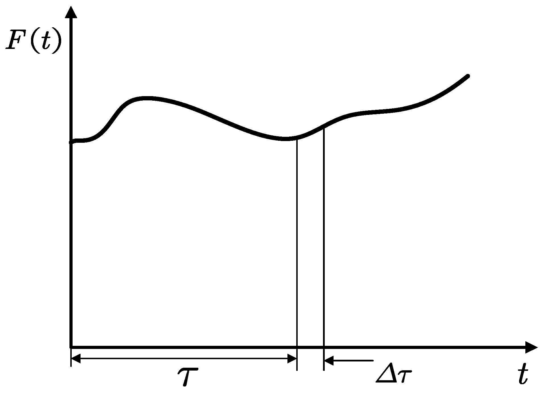
The aperiodic load excitation can be regarded as the weighted sum of several impulse excitation acting at different moments. The time width of each pulse tends to 0, and the value of at the corresponding moments can be taken as the weighted coefficient of each impulse, and thus can be regarded as the weighted sum of each impulse.
Figure 1 shows the conception of the impulse response theory (IRT).
As it was assumed that the dynamic system was a linear system, if the response of the system under the unit impulse excitation was solved, then the whole response can be solved according to the linear superposition principle. The response of a SDOF system with unit impulse was discussed under zero initial condition. The differential equation set of motion of the system was as follows:
In the above equation: was the unit impulse function, also known as the function, which was defined as follows:
In the above equation, the impulse width tended to be zero, and the amplitude tended to be ; however, the impulse was equal to 1.
The zero-initial condition in Equation (1) mean that the system was in static condition at the beginning and was suddenly affected by at the moment . As the time of action was extremely short, the instant time after the action was over can be written as . According to the theorem of momentum, the increase of momentum was equal to the impulse acting on the body; therefore: .
Assuming that the initial condition was , then the system obtained an initial velocity: . According to this assumption, the impact load can be decomposed into the superposition of several initial excitations. The problem expressed in Equation (1) can be converted to an initial value problem expressed as follows:
The parameters were set as follows:
It was assumed that the SDOF system was in the case of small damping ratio , the solution of Equation (3) was as follows:
The response of the system to unit impulse excitation was denoted as , and then the unit impulse response of the system can be expressed as follows:
For the impact load excitation , it can be regarded as a combination of a series of impulse excitation, and the impulse force at any time was . The system responded to the impulse was . According to the superposition principle of linear system, the whole response of the system was as follows:
When tended to be 0, the summation sign would become into integral; thus, the response of the system to the impact load can be expressed as follows:
In actual conditions, the impact load signal was discrete signal, such as . If the sampling interval of the signal was fixed, the time width of each pulse was also fixed, denoted as .
According to Equation (8), the integral form of continuous function can be transformed into the sum form of discrete function, as follows:
The discrete time integral of discrete impact load within the action time can be expressed as:
For a single excitation, the attenuation of the response within a time step can be expressed by the relative attenuation coefficient: . The damping ratio of steel structure was between 0.03 and 0.08, and the sampling frequency was 4096 Hz. Thus the attenuation coefficient corresponding to the first 100 Hz mode was about 0.9954, and the attenuation coefficient within 10 sample was about 0.9550.
As the attenuation coefficient was very close to 1, the amplitude of response can be regarded as constant in rising oscillation period. The amplitude in the rising oscillation period of each response was as follows:
The was the amplitude in rising oscillation period of each response (peak value), and the was the discrete time integral of the impact load. Equation (12) shows an approximate linear relationship between the two expressions:
To sum up, if the system parameters of the SDOF system are known, the response can be calculated according to the excitation. Reversely, the excitation can also be solved from the response.
2.1.2. Multiple Degree-Of-Freedom (MDOF) System
The same method can be extended to a MDOF system. A constant coefficient differential equation set with equations was used to describe the system with degrees of freedom, shown as the matrix equation:
In the above equation, are the mass matrix, damping matrix and stiffness matrix, respectively. refer to the generalized displacement, generalized speed and generalized acceleration vector, respectively. is the excitation force. The equation could also be expressed as follows:
The solution of the equation above can be written as , where is the general solution and is the particular solution.
- Particular solution
The particular solution of Equation (14) is as follows:
- General solution
According to the theory of vibration mechanics, the general solution of Equation (14) is as follows:
The solution of Equation (14) can be obtained by combining two solutions as follows:
Since the system had viscous damping, the free vibration would decay quickly; therefore, only the influence of the particular solution was considered in practice.
If the excitation was the discrete impact load, the expression of the response can be written as follows:
For each natural frequency , it can be regarded as a combination of SDOF systems.
The response with a frequency of within a sampling period can be approximated expressed as follows:
The amplitude in rising oscillation period of response can be expressed as follows:
Similar to the SDOF system, it was still an approximate linear relationship:
The above conclusions showed that the time integral of discrete impulse load was approximately linear with the peak value (amplitude of sine wave) in the rising oscillation period of response in MDOF system.
2.1.3. Conclusion
Within a given parameter range, the discrete time integral of the impact load had an approximate linear relationship with the peak value (amplitude of sine wave) in the rising oscillation period of response in both SDOF and MDOF systems. Theoretically, this linear relationship can be used to calculate the corresponding load according to the response given.
The accuracy of this method mainly depended on the accuracy of system parameter identification and the attenuation coefficient. If the identification of system parameters was more accurate, and the attenuation coefficient was closer to 1, the identification accuracy was higher.
The key point of the load identification method was to determine the system parameters, that is . Traditional methods typically determine each parameter by dynamic model or experiment, which is complicated and inaccurate. This paper used the neural network to determine the parameters of the system and establish a linear relationship between two signals.
2.2. BP Neural Network
The linear model of a neural network was a practical method to determine the unknown linear relationship. Theoretically, the mapping between two groups of data with linear relationship can be determined by a neural network. The discrete time integral of the impact load had an approximate linear relationship with the amplitude in the oscillation period of the response. The former was taken as the output and the latter as the input, and the neural network was used to establish the linear model between them.
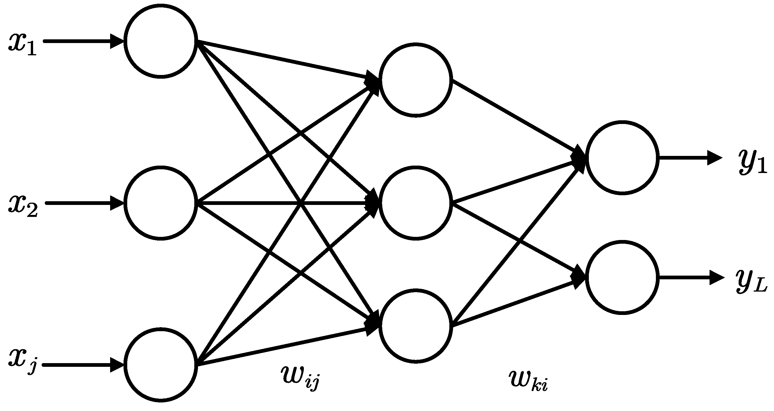
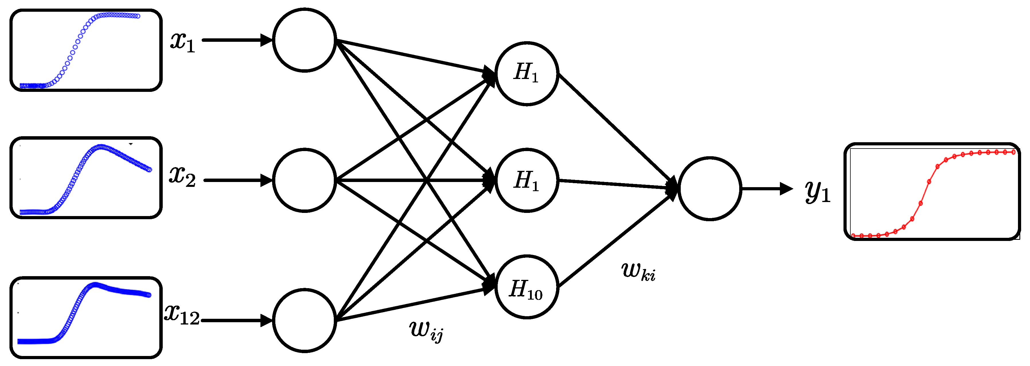
An Artificial Neural Network (ANN) was established by imitating the structure of the human neuron system, which had a high adaptive ability and learning ability [10]. A typical BP neural network was composed of an input layer, a hidden layer and an output layer. The signals transmitted forward and the errors transmitted reversely. When the result was inconsistent with the reference result, the error was propagated back, and the connection weights and thresholds of the neural network were adjusted according to the learning algorithm until the reference value was reached.
The structure of the neural network is as in Figure 2.
BP neural network consisted of input variables , hidden layers and output nodes .
The input calculation equation of the node in the hidden layer is as follows:
In the above equations, and , respectively, represent the input and output of the input layer node under the action of the sample , represents the connection weight between the input layer node and the hidden layer node, and represents the threshold of the hidden layer node.
If the error of output exceeds the set value, the error was fed back from the output layer, and the connection weights between the neuron nodes of each layer were modified until the error was less than the set value. The quadratic error for the output of any sample is expressed as:
The total error expression of the system is:
The main function of the ANN was the weight correction between the three layers.
- Correction of the connection weight between the output layer and the hidden layer
The connection weights between the neuron nodes of each layer were adjusted in the opposite direction of the gradient of the error function.
The adjustment expression of the connection weight can be obtained as:
Among the equation, and represent the expected result and the output value of the hidden layer node, respectively.
- Correction of the connection weights between the input layer and the hidden layer
In the same way, the modified expression of the connection weight between the hidden layer and the input layer can be obtained by the gradient of the error function:
Among the equation, and , respectively, represent the output of the hidden layer neuron node and the output of the output layer neuron node under the action of the sample .
Therefore, the weighting coefficient increment of the output layer node and the connection weight increment of the hidden layer node can be obtained under the action of the sample :
The connection weights of each layer of the neural network were adjusted to appropriate values until the error is no more than the set value.
3. Results
This chapter includes four sections, the experimental configuration Section 3.1, signal processing Section 3.2, neural network training and validation Section 3.3 and load identification Section 3.4.
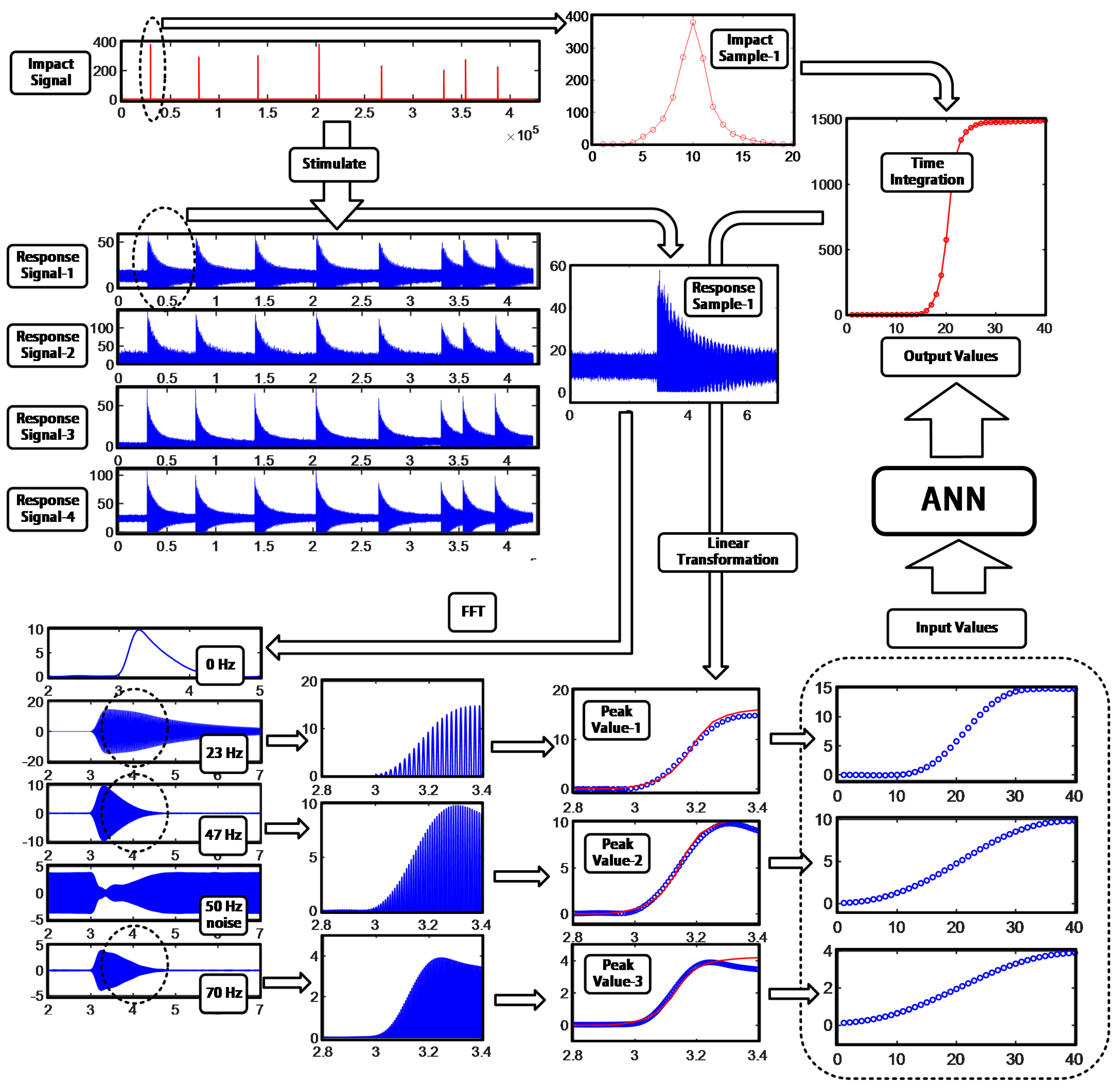
Figure 3 is the flow chart of signal processing and feature extraction. This figure contains the main content of the actual work of this paper.
3.1. Experiment Configuration
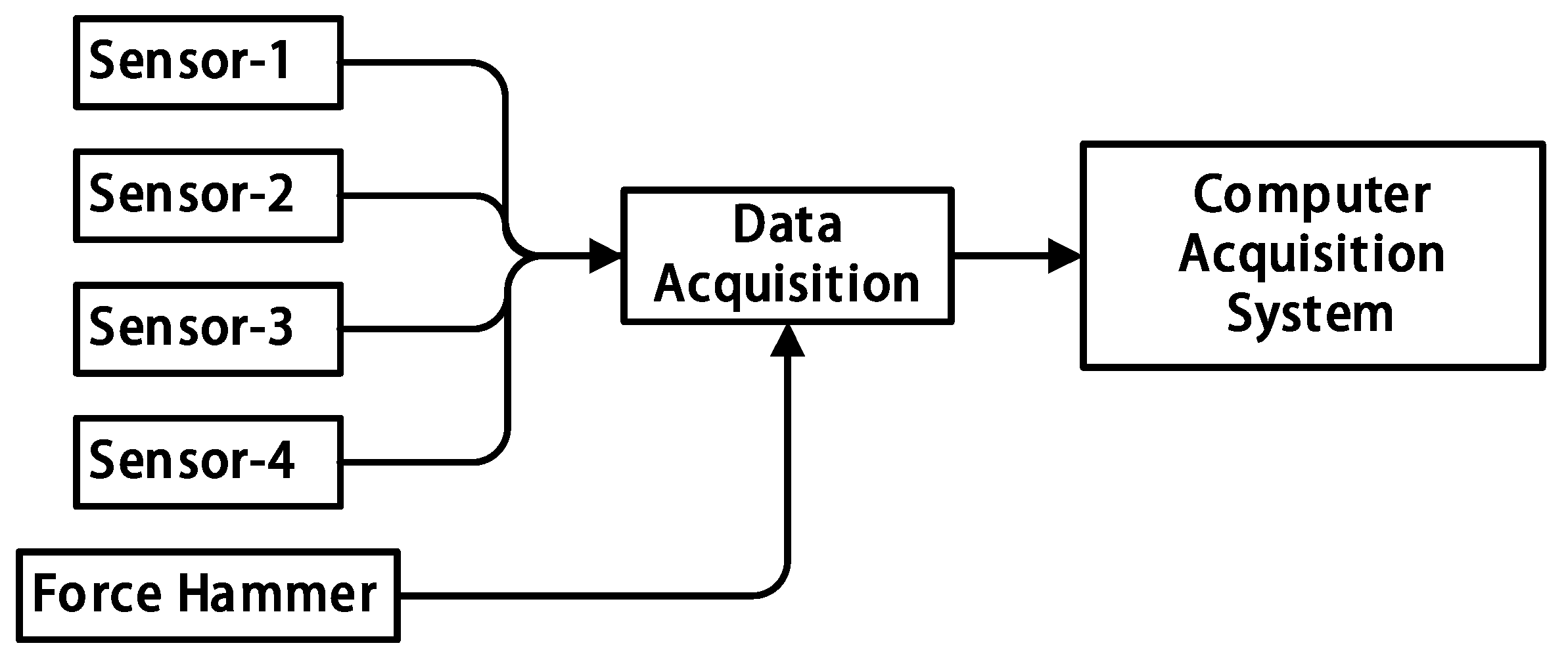
In this experiment, the excitation signal of the impact load was acquired by the force sensor on the force hammer, and the response signal was acquired by four sensors (strain rosette). The equipment included a force hammer (PCB086B20), strain rosette, power amplifier, digital acquisition and computer. Before the experiment, the strain rosette was firmly attached to the four measuring points on the steel structure, and the impact load was applied to the structure by the force hammer. The impact load signal was amplified by the power amplifier and then acquired by the digitizer. The response signals were acquired. The sampling frequency was set to 4096 Hz.
The connection diagram of each issue is shown in Figure 4.
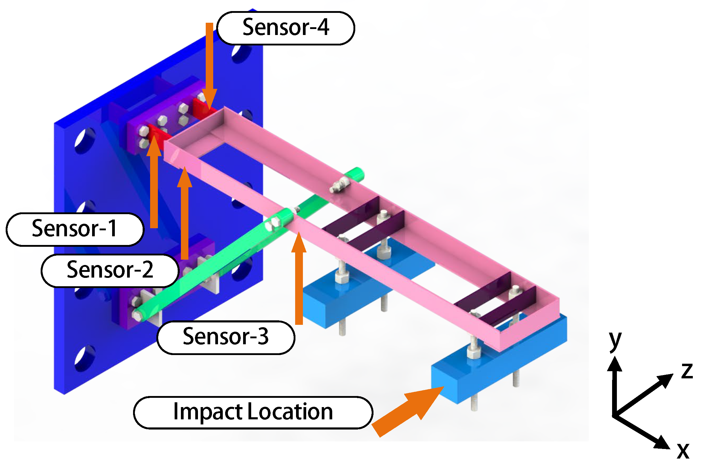
The experimental structure used in this article was a steel cantilever beam with two supporting bars. The density was 7850 kg/m3, and the elastic modulus was 210 Gpa. The main beam was made of 30 × 30 mm angle steel with the thickness of 3 mm; the middle is connected by partition frame with the thickness of 3 mm. The actual structure is shown in Figure 5.
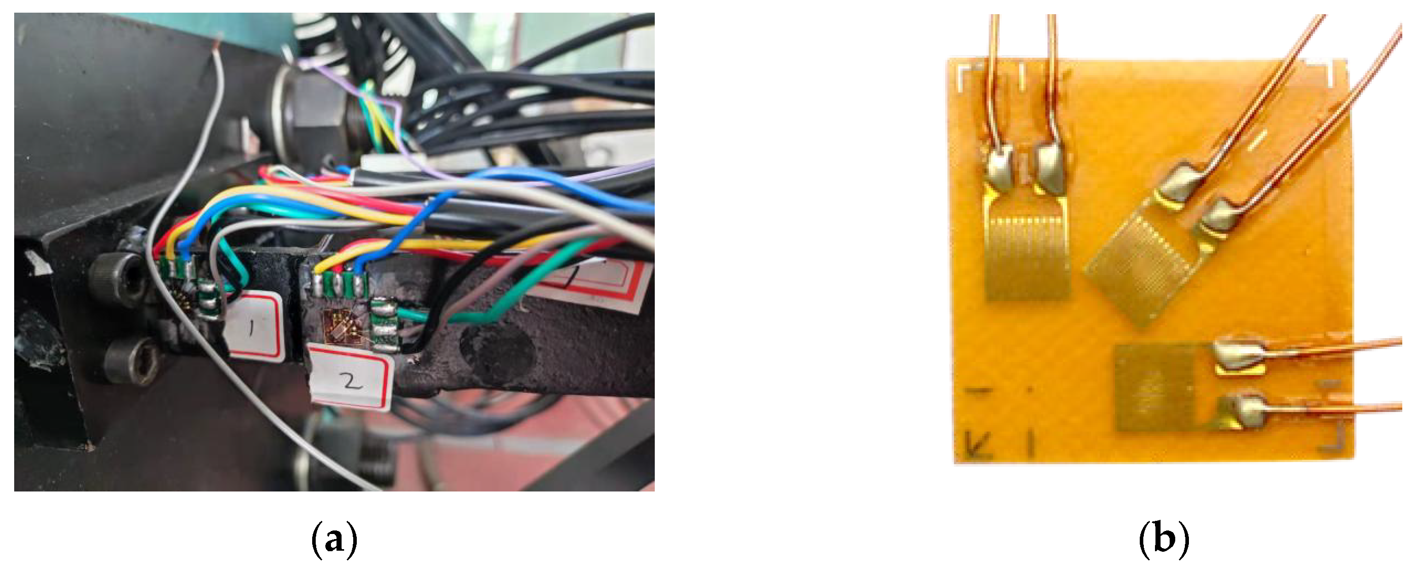
Figure 6 shows the details of the strain rosette used in this experiment.
Table 1 listed the exact location of the force hammer and four sensors (strain rosette) in the space coordinate system.
3.2. Signal Processing
This part includes the design of the digital filter, discrete-time integration of impact load and extraction of peak value (amplitude of sine wave) in the rising oscillation period of response.
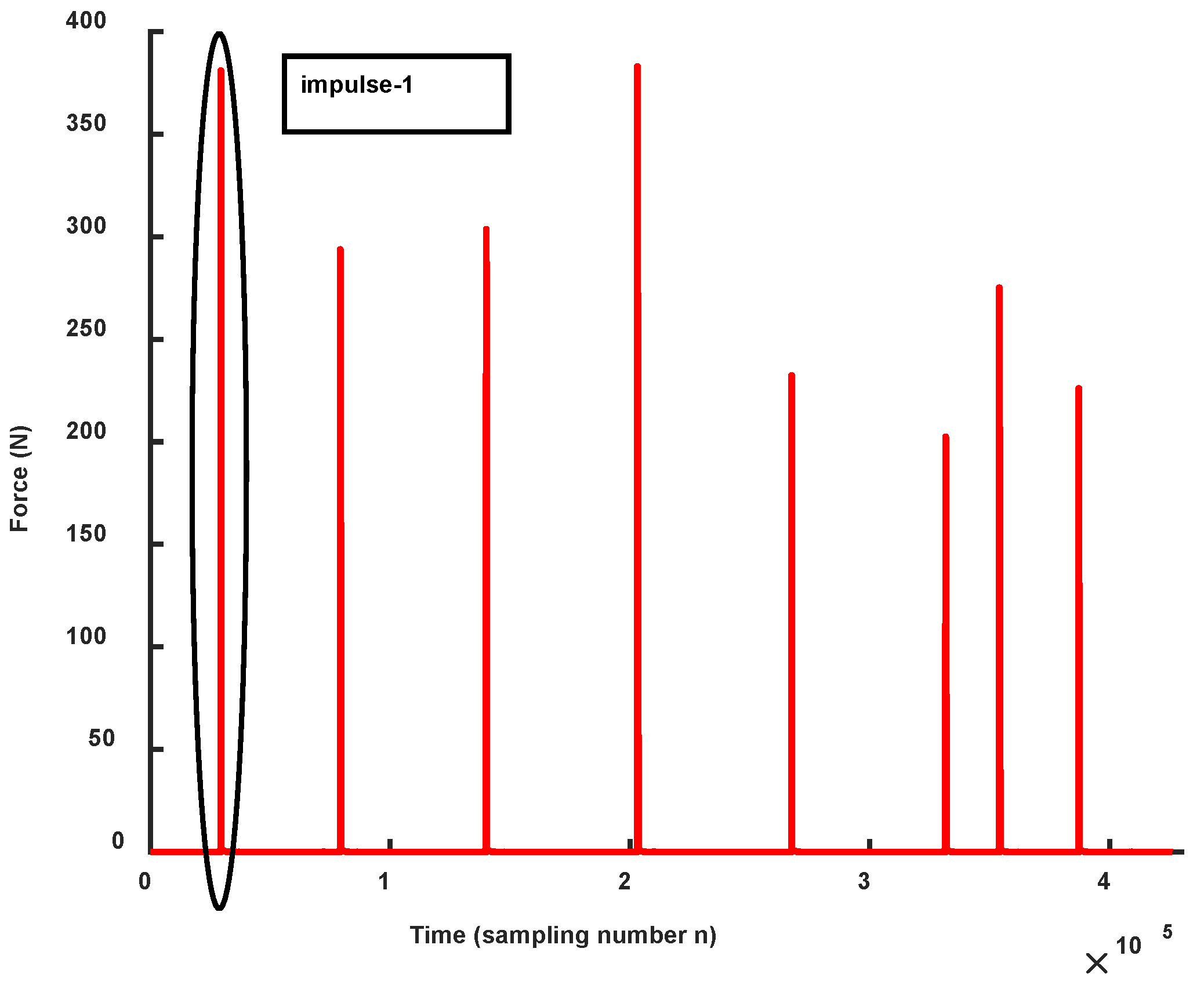
Figure 7 shows the impact load records throughout the experiment. The time interval between the last three impact loads was too short for the response to decay completely. Therefore, the last three sets of data were not used in the following signal processing. The signal 1 in Figure 7 is taken as an example.
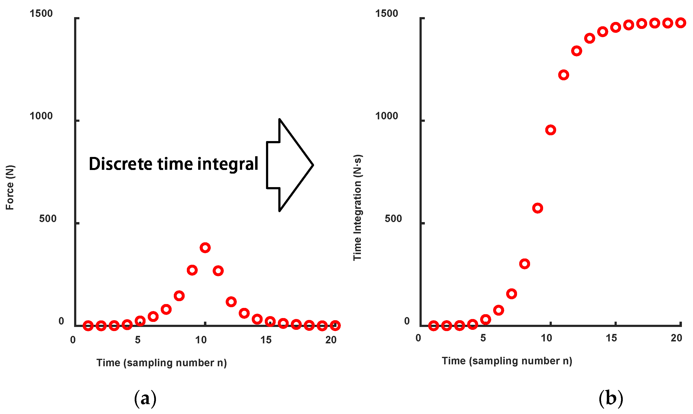
Figure 8a shows the actual time–force history of the impact load 1, which was a discrete signal. Figure 8b shows the discrete time integral of impact load 1, which was also a set of discrete values. The specific calculation equation of discrete integral value is Equation 10.
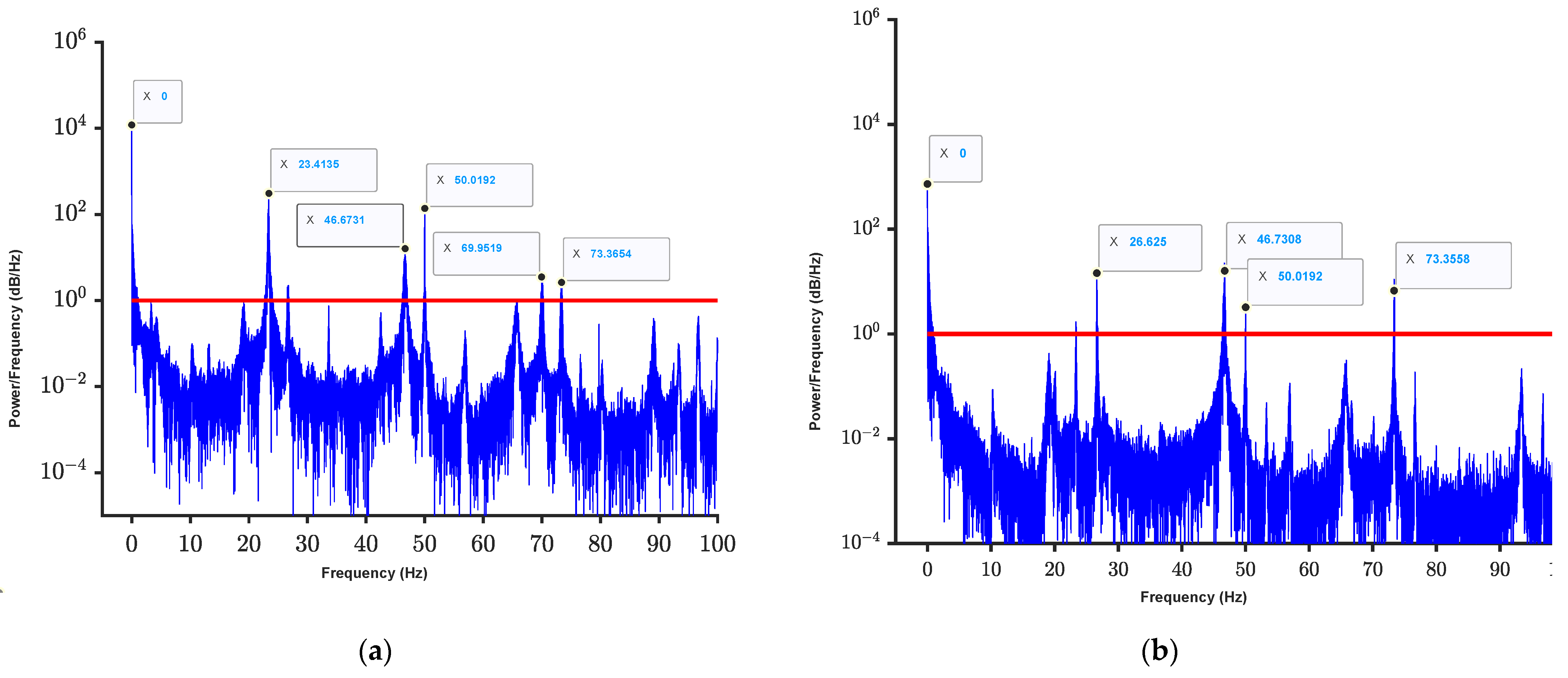
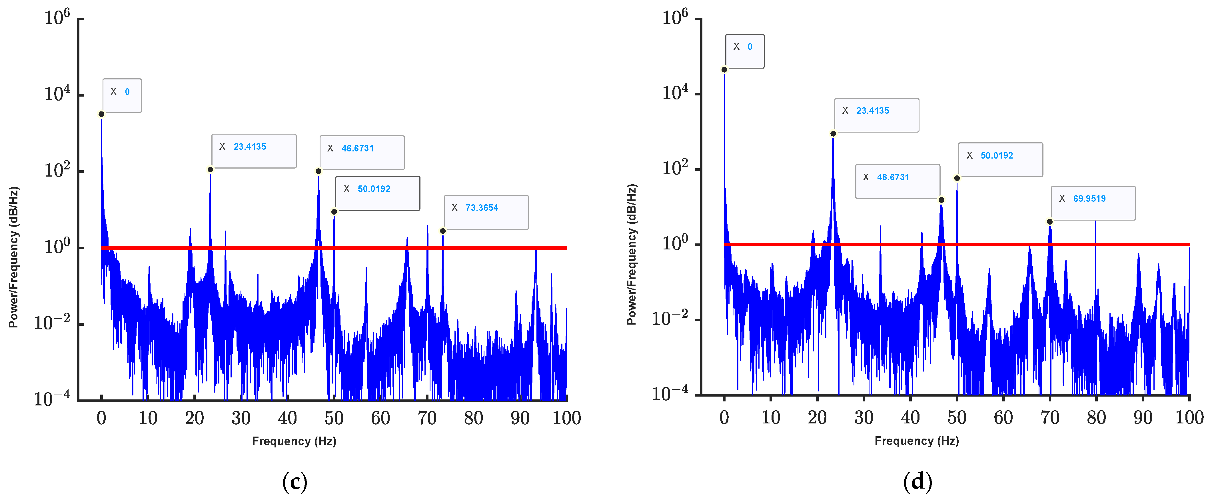
According to the response solution of the MDOF system, the response signals of each sensor contain multiple natural frequencies. Figure 9 shows the power spectral density (PSD) analysis results of four response from four sensors.
The PSD shows that there were several similar frequencies of four sensors. The natural frequencies of the frame structure in Table 1 was obtained from the modal experiment.
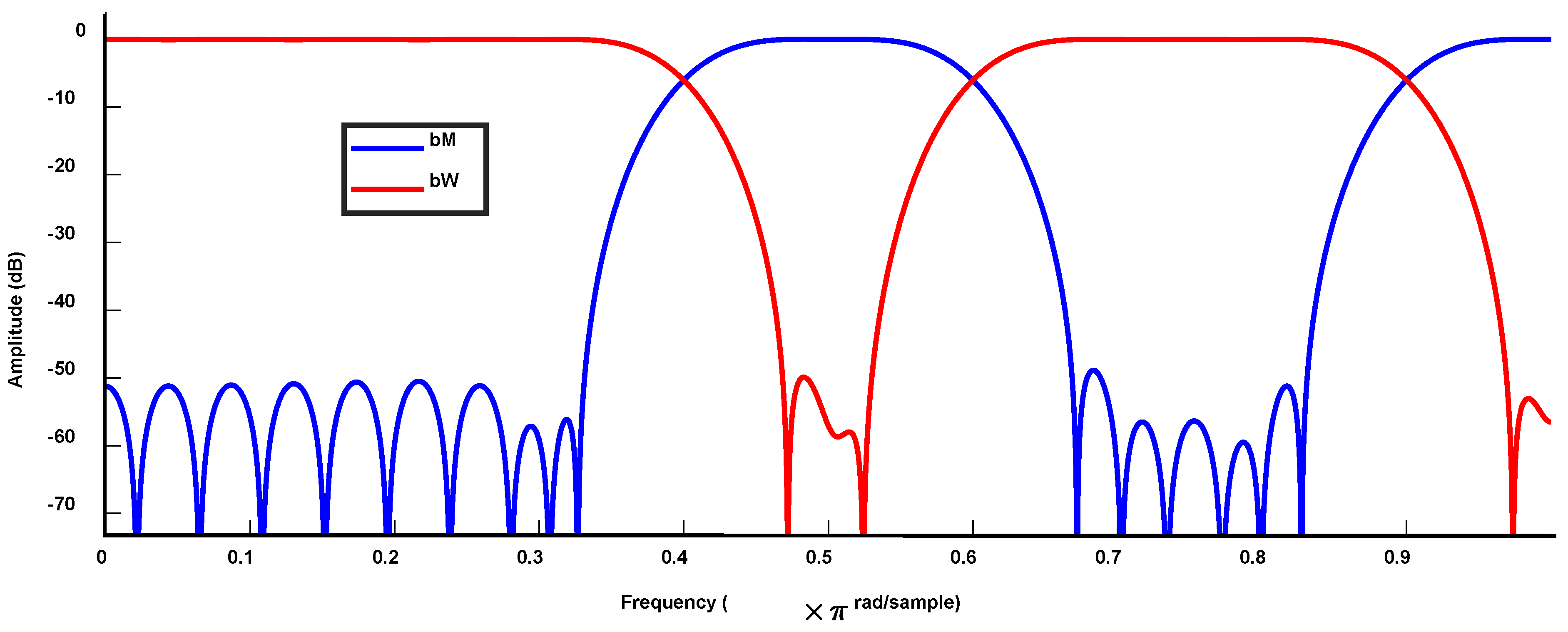
According to Figure 9 and Table 2, the primary modes were order 1, order 3 and order 5. Considering that the impact direction was the Z direction, the proportion of the vertical bending mode (order 2) was not significant. There was also a frequency component of 50 Hz. In order to obtain the response of each frequency component individually, a bandpass digital filter was designed as shown in Figure 10.
The filter was a FIR1 type bandpass filter. By filtering the primary frequencies individually, the response signals at each frequency were obtained. The parameters of the filter are shown in Table 3.
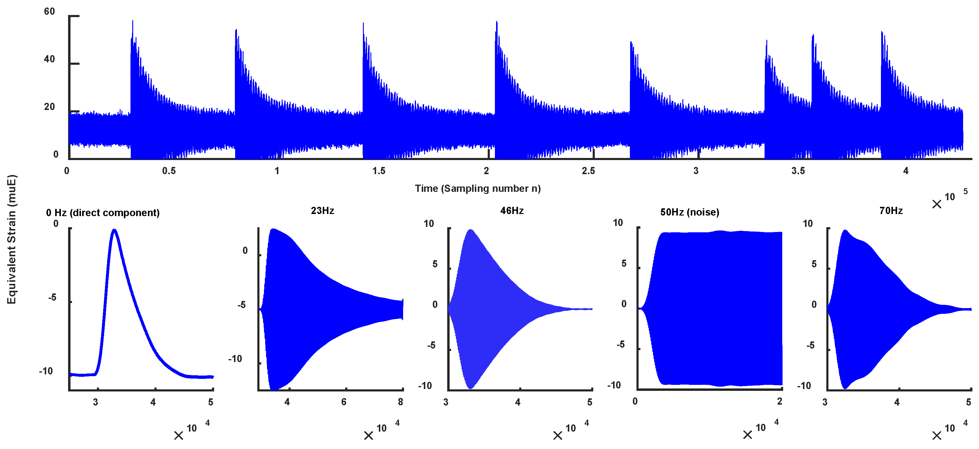
Taking Response 4 as an example, the result is shown in Figure 11.
Figure 11 shows that the 0 Hz component was the fundamental motion without oscillation. The frequency component of 50 Hz did not change with the load; thus, it was noise.
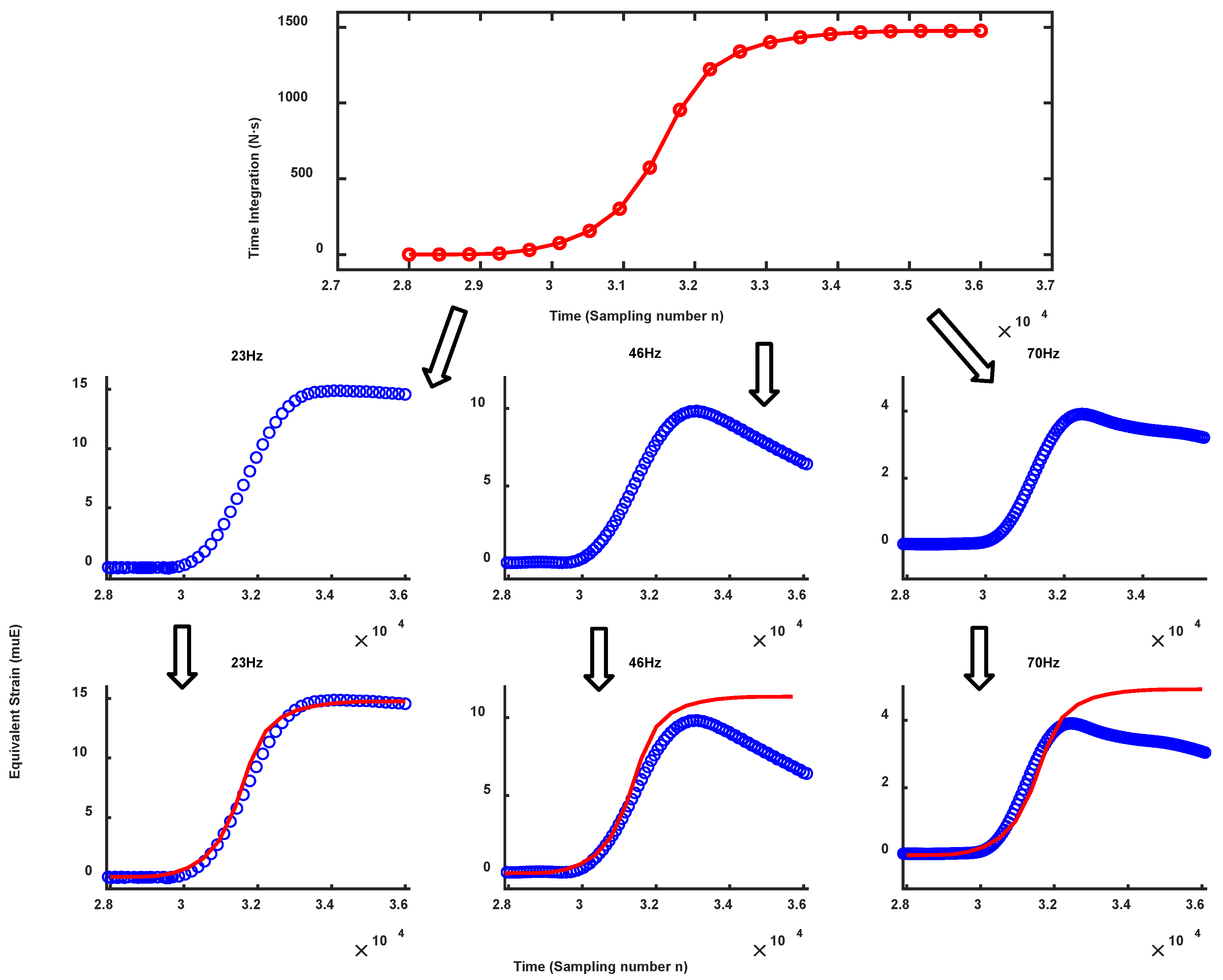
In conclusion, three frequencies of 23, 46 and 70 Hz were selected as identification response signals as shown in Figure 12.
Figure 12 shows that, through linear transformation, there was indeed a linear relationship between the discrete time integral of the load and the peak value (amplitude of sine wave) in the rising oscillation period of the response. This also confirmed the feasibility of the previous theoretical assumptions. The impact load can be solved according to the linear combination of the response in three frequencies. The peak value (amplitude of sine wave) in the oscillation rising period of the response at three frequencies were extracted as a group of outputs.
The above analysis was given by taking sensor 4 as an example. The situation was similar for other three sensors. A total of 12 sets of data from all four sets of rosettes were extracted to construct the input sample data of the neural network.
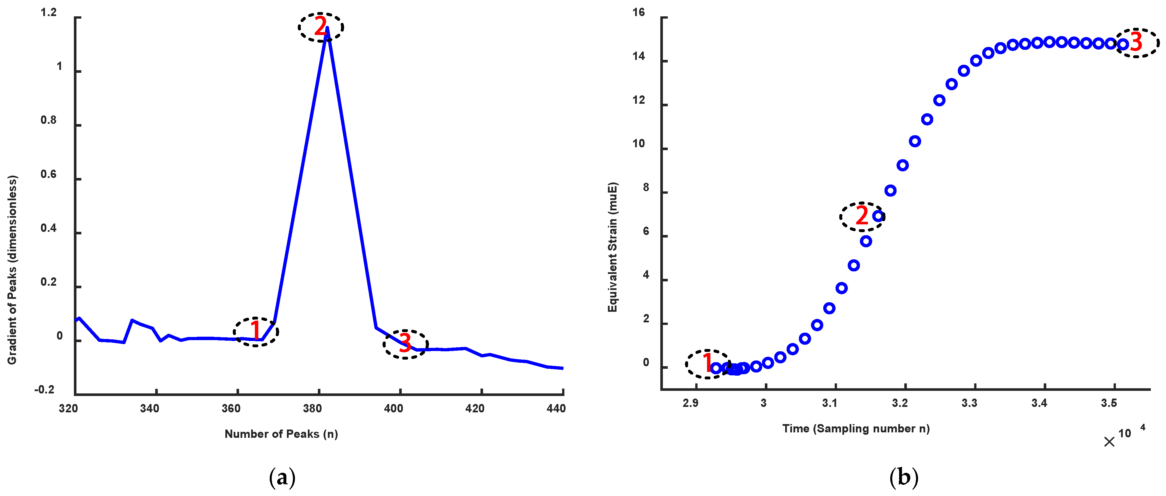
To ensure that the maximum value of each group of differential peaks can be extracted, discrete-time differentiation was performed on each peak value (amplitude of sine wave), and Figure 13a was obtained, and the data between the differential maximum point and the left and right 0 points were taken as a set of response samples as shown in Figure 13.
3.3. The Training of the BP Neural Network
The linear relationship between the input and output was constructed through the linear model of the neural network. The structure diagram of the BP neural network used in this paper is shown in Figure 14. It contained 12 inputs, 1 output and 10 hidden layers. The network was trained with the Levenberg–Marquardt backpropagation algorithm.
The performance of the neural network in the training process is shown in Table 4.
As shown in Table 4, the MSE of the three sets of data was small, while the R was close to 1 which meant a strong linear relationship between the input and output. This result also confirmed that the theory proposed in this paper was correct and that the processing of the response signal was feasible.
3.4. Impact Load Identification
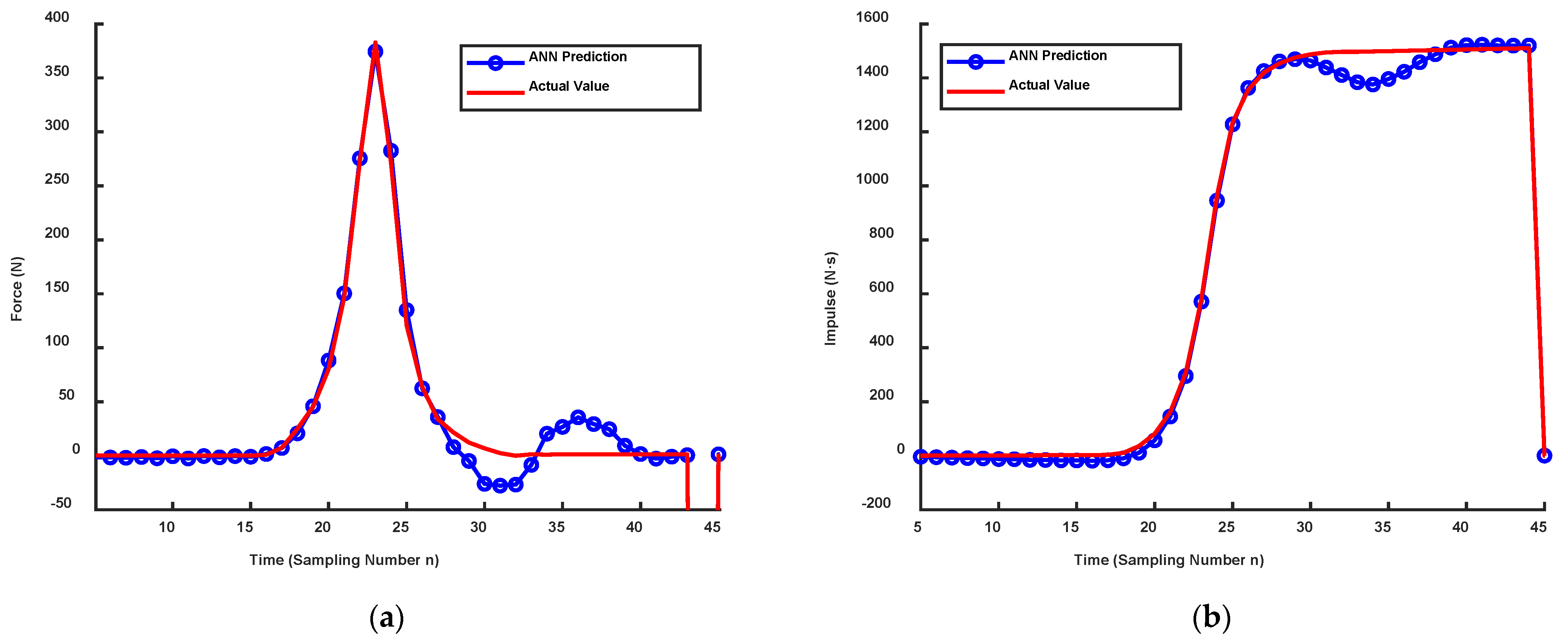
This section used the neural network established before to proceed load identification. The recognition results are shown in Figure 15.
Figure 15a shows the time–force history of load identification and actual value, and Figure 15b shows the time–impulse history of identification and actual value. In practical applications, the maximum amplitude and impulse of the impact load were always given more attention. Table 5 lists the statistics value of the identification results.
Table 2 shows that the identification method had high accuracy. The error between the actual maximum amplitude of impact load and the identification value was 2.22%. The error between the actual equivalent impulse and the identification was 0.67%. These results show that the neural network established in this paper had good performance and that the signal feature extraction method had high credibility.
4. Discussion
In this paper, an impact load identification method based on impulse response theory (IRT) and BP neural network was proposed. By extracting the peak value (amplitude of sine wave) in the rising oscillation period of the response, it transformed the excitation and response signals into the same length. The ANN was used to verify the linear relationship between the time integration of load and peak value of the response, the results showed that there was a strong linear relationship between them. In this article, we did not take the attenuation of response in the rising period into consideration; however, the results were still ideal. That meant the damping ratio of the structure was relatively tiny.
The identification results shown in Figure 15 still had some errors in the end of the signal. The reason might be that the number of training samples was not sufficient. To improve the performance of the ANN, some methods to select the training data should be used. The impulse response theory (IRT) was the basic theory of our manuscript, and the experiment results showed that the theory was effective in this condition. The precondition of this theory was that there was no plastic deformation in structure. If there was plastic deformation, the IRT was not suitable, and the stress wave must be taken into consideration.
Reviewing the research process of this paper, there were still some aspects worth researching in the further. From the experimental perspective: (1) In the response signal, there was a noise mainly at 50 Hz and at the doubling frequencies (100, 150, 200 Hz, etc.). The noise was electric network noise, mainly caused by the absence of an electromagnetic shielding wire. (2) Some intervals of impact were too short, which resulted that the former response signals superposed with the latter ones.
From theory perspective: (1) Only the peak value (amplitude of sine wave) of the response signal was used, which resulted in a certain waste. How to extract more features from other parts of the response signal is worth researching. (2) As the sampling time interval was too short, the actual maximum amplitude of the impact was likely to be missed. Identifying the actual maximum of the impact is a valuable issue.
Though there are some aspects waiting to be explored, the results of this paper have both theoretical and practical value. The neural network tool method was introduced into the field of impact load identification, and a new way to extract signal features was established. A neural network was used to identify the linear parameters of the system, which was more efficient and faster than traditional methods. The validation results showed that the method had high accuracy and practical application potential.
Author Contributions
Conceptualization, methodology, software, writing—original draft preparation and writing—review and editing, D.H.; experiment data, L.C. and X.Y.; supervision, project administration and funding acquisition, Y.G. All authors have read and agreed to the published version of the manuscript.
Funding
This research is a project funded by the Nanjing University of Aeronautics and Astronautics: National Key Laboratory of Rotorcraft Aeromechanics (61422202104) and Priority Academic Program Development of Jiangsu Higher Education (PAPD).
Institutional Review Board Statement
Not applicable.
Informed Consent Statement
Not applicable.
Data Availability Statement
Not applicable.
Conflicts of Interest
The authors declare no conflict of interest.
References
- Tian, Y.; Xing, S.; Zhang, Z.; Zheng, H. Load Identification of Gearbox Based on Radial Basis Function Neural Networks. J. Vib. Meas. Diagn. 2004, 24, 16–18+74. [Google Scholar] [CrossRef]
- Tian, Y.; Xing, S.; Zheng, H. Load identification of the gearbox based on Elman networks. J. Vib. Eng. 2006, 19, 114–117. [Google Scholar] [CrossRef]
- Staszewski, W.J.; Worden, K.; Wardle, R.; Tomlinson, G.R. Fail-safe sensor distributions for impact detection in composite materials. Smart Mater. Struct. 2000, 9, 298–303. [Google Scholar] [CrossRef]
- Ghajari, M.; Sharif-Khodaei, Z.; Aliabadi, M.H.; Apicella, A. Identification of impact force for smart composite stiffened panels. Smart Mater. Struct. 2013, 22, 085014. [Google Scholar] [CrossRef] [Green Version]
- Wang, J.; Wang, C.; Lai, X. MIMO SVM Based Uncorrelated Multi-source Dynamic Random Load Identification Algorithm in Frequency Domain. J. Comput. Inf. Syst. 2015, 11, 198–207. [Google Scholar]
- Wang, J.G.; Zhang, J.; Wang, Y.J.; Fang, X.Y.; Zhao, Y.X. Nonlinear identification of one-stage spur gearbox based on pseudo-linear neural network. Neurocomputing 2018, 308, 75–86. [Google Scholar] [CrossRef]
- Cheng, G.; Ren, F.; Yang, Z. Study on Load Identification of Double Span Rotor System. Coal Technol. 2018, 37, 278–280. [Google Scholar] [CrossRef]
- Zheng, S.; Guo, T.; Dong, H.; Song, Z. Load identification of piezoelectric structures by using genetic algorithm and finite element analysis. Chin. J. Comput. Lmechanics 2009, 26, 330–335. [Google Scholar]
- Cao, X.; Sugiyama, Y.; Mitsui, Y. Application of artificial neural networks to load identification. Comput. Struct. 1998, 69, 63–78. [Google Scholar] [CrossRef]
- Cooper, S.B.; DiMaio, D. Static load estimation using artificial neural network: Application on a wing rib. Adv. Eng. Softw. 2018, 125, 113–125. [Google Scholar] [CrossRef]
- Ren, S.; Chen, G.; Li, T.; Chen, Q.; Li, S. A Deep Learning-Based Computational Algorithm for Identifying Damage Load Condition: An Artificial Intelligence Inverse Problem Solution for Failure Analysis. Comput. Modeling Eng. Sci. 2018, 117, 287–307. [Google Scholar] [CrossRef] [Green Version]
- Chen, G.R.; Li, T.G.; Chen, Q.J.; Ren, S.F.; Wang, C.; Li, S.F. Application of deep learning neural network to identify collision load conditions based on permanent plastic deformation of shell structures. Comput. Mech. 2019, 64, 435–449. [Google Scholar] [CrossRef]
- Zhang, Z.; Zhang, H.; Chen, Y.; Li, Z.; Fu, Z. Load identification method of track driving system based on genetic neural network. J. Vib. Shock. 2022, 41, 54–61+89. [Google Scholar]
- Yang, T.; Yang, Z.; Liang, S.; Kang, Z.; Jia, Y. Time-frequency feature extraction and identification of stationary random dynamic load using deep neural network. Acta Aeronaut. Astronaut. Sin. 2022, 37, 98–108. [Google Scholar]
- Xia, P.; Yang, T.; Xu, J.; Wang, L.; Yang, Z. Reversed time sequence dynamic load identification method using time delay neural network. Acta Aeronaut. Et Astronaut. Sin. 2022, 42, 389–397. [Google Scholar] [CrossRef]
Figure 1.
F(t) can be decomposed into discrete impulse excitations.

Figure 2.
Topological structure of a typical back propagation neural network.

Figure 3.
The whole process of the signal processing and featuring extraction.

Figure 4.
The configuration of the experiment system.

Figure 5.
3D model of the steel frame structure including the location of four sensors and impact load.
Figure 5.
3D model of the steel frame structure including the location of four sensors and impact load.

Figure 6.
(a) The real configuration of one sensor (strain rosette). (b) The specific structure of one strain rosette.
Figure 6.
(a) The real configuration of one sensor (strain rosette). (b) The specific structure of one strain rosette.

Figure 7.
Load-time history of all impact signals.

Figure 8.
(a) Load-time history of impact load 1 (after zoom in). (b) Load-time discrete integration of impact load 1.
Figure 8.
(a) Load-time history of impact load 1 (after zoom in). (b) Load-time discrete integration of impact load 1.

Figure 9.
Power Spectral Density (PSD) of four response signals from four strain rosettes. (a) Response Signal-1; (b) Response Signal-2; (c) Response Signal-3; and (d) Response Signal-4. The red line in each represented the standard amplitude of the PSD.
Figure 9.
Power Spectral Density (PSD) of four response signals from four strain rosettes. (a) Response Signal-1; (b) Response Signal-2; (c) Response Signal-3; and (d) Response Signal-4. The red line in each represented the standard amplitude of the PSD.


Figure 10.
The example amplitude response of the FIR-I filter (Attenuates normalized frequencies below 0.4π rad/sample and between 0.6π and 0.9π rad/sample).
Figure 10.
The example amplitude response of the FIR-I filter (Attenuates normalized frequencies below 0.4π rad/sample and between 0.6π and 0.9π rad/sample).

Figure 11.
The response signal–4 was decomposed into several frequencies. (0, 23, 46, 50 and 70 Hz).
Figure 11.
The response signal–4 was decomposed into several frequencies. (0, 23, 46, 50 and 70 Hz).

Figure 12.
Schematic diagram of linear relation of load–time discrete integration and the peak value (amplitude of sine wave) of the oscillation period.
Figure 12.
Schematic diagram of linear relation of load–time discrete integration and the peak value (amplitude of sine wave) of the oscillation period.

Figure 13.
(a) The gradient of the peak value (amplitude of sine wave). (b) The value of the oscillation period. The point marked number 1 and 3 represented the point that the gradient equals to zero, the point marked number 2 represented the point that the gradient reached the maximum.
Figure 13.
(a) The gradient of the peak value (amplitude of sine wave). (b) The value of the oscillation period. The point marked number 1 and 3 represented the point that the gradient equals to zero, the point marked number 2 represented the point that the gradient reached the maximum.

Figure 14.
The structure of the BP neural network used in this article.

Figure 15.
(a) The identification results of the load–time history. (b) The identification result of the impulse–time history.
Figure 15.
(a) The identification results of the load–time history. (b) The identification result of the impulse–time history.


Table 1.
Location of four sensors (rosette) and impact load (force hammer).
| Item | XYZ Location (mm) |
|---|---|
| Sensor-1 | (0.0, 0.0, 0.0) |
| Sensor-2 | (41.6, 3.2, −13.8) |
| Sensor-3 | (326.7, 3.2, −13.8) |
| Sensor-4 | (0.0, 0.0, 90.2) |
| Impact | (607.6, −73.8, 156.2) |
Table 2.
The natural frequency and mode of the actual model.
| Order | Natural Frequency (Hz) | Mode of Vibration |
|---|---|---|
| 1 | 23.3 | Bending (horizontal) |
| 2 | 33.5 | Bending (vertical) |
| 3 | 45.7 | Torsion (Y axis) |
| 4 | 67.3 | Torsion (X axis) |
| 5 | 74.3 | Torsion (Z axis) |
Table 3.
The frequency and the filter band for designing the FIR-I filter.
| Frequency (Hz) | Filter Band (Hz) |
|---|---|
| 0 | (0, 0.1) |
| 23 | (23, 24) |
| 46 | (46, 47) |
| 50 | (49, 50) |
| 70 | (69, 70) |
Table 4.
Performance of the neural network during training and validation.
| Situation | Sample Number | MSE I | R II |
|---|---|---|---|
| Training | 84 | 2.74376 | 0.999996 |
| Validation | 18 | 7.35701 | 0.999994 |
| Testing | 18 | 7.62322 | 0.999992 |
I Regression R Values measure the correlation between outputs and targets. An R value of 1 means a close relationship, and 0 is a random relationship. II Mean Squared Error (MSE) is the average squared difference between outputs and targets. Lower values are better. Zero means no error.
Table 5.
Relative error of the impact load identification results.
| Frequency (Hz) | ANN Prediction | Actual Value | Relative Error |
|---|---|---|---|
| Maximal Force(N) | 374.40 | 382.90 | 2.22% |
| Equivalent Impulse (N·s) | 1520.00 | 1510.00 | 0.67% |
Publisher’s Note: MDPI stays neutral with regard to jurisdictional claims in published maps and institutional affiliations. |
© 2022 by the authors. Licensee MDPI, Basel, Switzerland. This article is an open access article distributed under the terms and conditions of the Creative Commons Attribution (CC BY) license (https://creativecommons.org/licenses/by/4.0/).
Share and Cite
MDPI and ACS Style
Huang, D.; Gao, Y.; Yu, X.; Chen, L. The Feature Extraction of Impact Response and Load Reconstruction Based on Impulse Response Theory. Machines 2022, 10, 524. https://0-doi-org.brum.beds.ac.uk/10.3390/machines10070524
AMA Style
Huang D, Gao Y, Yu X, Chen L. The Feature Extraction of Impact Response and Load Reconstruction Based on Impulse Response Theory. Machines. 2022; 10(7):524. https://0-doi-org.brum.beds.ac.uk/10.3390/machines10070524
Chicago/Turabian StyleHuang, Dawei, Yadong Gao, Xinyu Yu, and Likun Chen. 2022. "The Feature Extraction of Impact Response and Load Reconstruction Based on Impulse Response Theory" Machines 10, no. 7: 524. https://0-doi-org.brum.beds.ac.uk/10.3390/machines10070524
Note that from the first issue of 2016, this journal uses article numbers instead of page numbers. See further details here.