Fault Detection for High-Speed Trains Using CCA and Just-in-Time Learning

Abstract

Online monitors of the running gears systems of high-speed trains play critical roles in ensuring operational safety and reliability. Status signals collected from high-speed train running gears are very complex regarding working environments, random noises and many other real-world constraints. This paper proposed fault detection (FD) models using canonical correlation analysis (CCA) and just-in-time learning (JITL) to process scalar signals of high-speed train gears, named as CCA-JITL. After data preprocessing and normalization, CCA transforms covariance matrices of high-dimension historical data into low-dimension subspaces and maximizes correlations between the most important latent dimensions. Then, JITL components formulate local FD models which utilize subsets of testing samples with larger Euclidean distances to training data. A case study introduced a novel system design of an online FD architecture and demonstrated that CCA-JITL FD models significantly outperformed traditional CCA models. The approach is applicable to other dimension reduction FD models such as PCA and PLS.

1. Introduction

In the past twenty years, high-speed railway systems are gradually becoming one of the most popular transportation services because of their significant advantages in speed and energy efficiency [1,2,3]. The running gears are critical parts to ensure the safety of high-speed train operations. To precisely detect the real-time health status of running gears is very challengeable. In reality, sensor signals of running gears in high-speed trains have a very high degree of complexity, for instance, messy signals from bogie, bearing temperature, gear temperature, working environments and random noises. Moreover, there are only small-scale historical failure data available among large volumes of monitoring data streams. Incomplete training resources might easily raise detection errors.

With the rapid development of train sensor technology, data-driven FD methods have been well studied in the last century. Many multivariate statistical methods have been widely applied in the fault detection fields [4,5,6], for example, principal component analysis (PCA), partial least squares (PLS) and CCA. PCA was one of the earliest dimensionality reduction methods to process high-dimension signal data for FD purposes [7,8]. PCA projects high-dimension input data into low-rank subspaces while retaining the main information of the original data within a few top latent dimensions. Moreover, PCA FD models are derived from a large scale of normal status signals and generate fault alarm thresholds for incoming error signals. PLS and CCA are widely utilized to develop advanced FD models [6,9,10]. PLS decomposes the covariance matrices of two sets of variables into relational subspaces and residual subspaces. Then, the regression analysis to covariance structure estimates the multi-direction of one set of variables that explains the maximum multidimensional variance direction of another set of variables. CCA identifies linear combinations between two groups of variables to maximize the overall group correlation. Multi-set CCA resolved feature fusion of multiple groups of variables [11].

Chen and Ding [12] designed a general CCA-based FD infrastructure for non-Gaussian processes which aimed to boost the fault detection rate (FDR) under an acceptable false alarm rate (FAR). Peng and Ding [13] have proposed CCA-based distributed monitoring processes within partly-connected networks, which reduced communication costs and risks and avoided a significant drop in system performance. Chen and Chen [6] introduced a single-side CCA (SsCCA) model with promising FD performance using single-side neural networks. Chen and Li [14] had proposed a stacked approach, so called neural network-aided canonical variate analysis (SNNCVA), which showed satisfactory FD performance for nonlinear datasets. Garramiola and Poza [15] introduced a data-driven approach of fault diagnosis to build hybrid fusion models to detect, isolate and classify sensor faults. Kou and Qin [16] extended fault diagnosis methodology into tensor space to deal with multi-sensor data with high precision and convergence speed. Zhao and Yan [17] provided a comprehensive review which summarized state-of-the-art deep learning (DL) technologies applied on machine health monitoring (MHM). Niu and Xiong [18] proposed a novel fault Petri net fault detection and diagnosis (FDD) model to analyze signals of speed sensors of high-speed trains. Fu and Huang [19] proposed a fault diagnosis method based on the long-short-term memory (LSTM) recursive neural network (RNN) to reduce the steps of signal preprocessing and optimize prediction accuracy. Cheng and Guo [20] designed a real-time prediction framework for running state of running station based on multi-layer BRB and priority scheduling strategy. Guan and Huang [21] created a particle swarm optimization algorithm based on wavelet variation and a least squares support vector machine to avoid falling into local extremum problems. Sayyad and Kumar [22] introduced a survey to review service life prediction technologies of real-time health monitors of cutting tools from perspectives of modeling, systems, data sets and research trends. Capriglione and Carratu [23] proposed an FD method using a nonlinear autoregressive with Exogenous Inputs (NARX) neural network as a residual generator for online FD of travel sensors. Shabanian and Montazeri [24] proposed an online FD and diagnosis algorithm based on the neural fuzzy, and adaptive analytic method and neural network to track faults online.

JITL technologies involve collecting the most relevant samples as training data for online query and making predictions of local modeling running time [25,26,27]. Compared with similar samples in historical databases, the signal status of online query could be possibly acquired in real time. Robust JITL strategies to leverage the weights of high leakage points of signals such as outliers had been successfully applied to the FD tasks [28]. A simulation study showed that the combined JITL-PCA models outperformed PCA in the analyzing of nonlinear signals [26]. In addition, neural network methods and the stochastic hidden Markov model (HMM) were studied to improve FD performance of dynamic systems [29,30].

Motivated by the previous studies, we designed a novel CCA-JITL model to analyze real-time signals from running gears of high-speed trains. The model was built and testified using real-world datasets. The algorithm split the data input into two groups and verified the system performance by group comparison The evaluation demonstrated that the accuracy of FD detection was significantly improved. The algorithm detects the data in groups and verifies the two groups of results, and the proposed system infrastructure was also applicable to enhance PCA and PLS FD models.

The rest of this article is content as follows. Section 2 gives introduction the structure of running gears system, experiment design and datasets. Section 3 presents theoretical foundations of the proposed method. Section 4 presents evaluation results of a FD use case and discussion of the results. Finally, Section 5 summarizes this paper study.

2. Preliminaries

This section introduces the mechanical structure of a running gear system in a high-speed train. In this study, signal faults mainly caused by parts were selected as FD targets. Then, the research goals and problem statements of system design were discussed.

2.1. Introduction of a Running Gears System of a High-Speed Train

The running gear system is an important system that affects the smooth running of high-speed trains. It improves the traction performance of high-speed trains and has the functions of generating power, buffering and supporting. The running gears system of high-speed trains include many complicated parts such as the axle box, traction drive, detection sensor, and spring device. Any malfunction from these parts may cause the carriage to shake during running and result in unpredictable consequences.

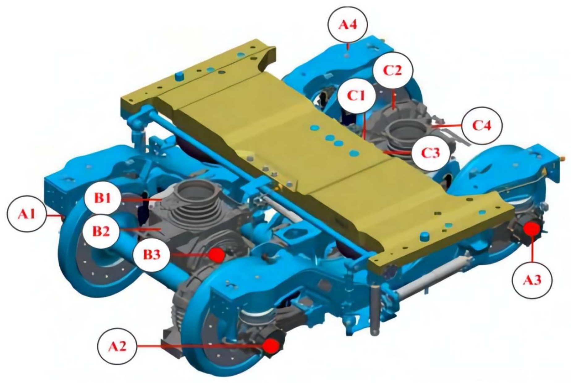
This paper aimed to analyze the running gears model and establish a data-driven FD model. The running gears system has such a multi-level complex structure. Therefore, it is difficult to build an FD model. As shown in Figure 1, many temperature sensors are arranged inside the gears. The test points of temperature sensors, for example, $A1$–$A4$ for axle box bearing temperature measuring point, $B1$–$B3$ for motor temperature measuring point, and $C1$–$C4$ for gear box temperature are shown in Figure 1 [31].

2.2. Fault Description

The running gears system is equipped with many sensors to keep track of the actual status. The real data used in this study is based on data collected by a railway department in a specific year and then classified and processed to obtain the fault signals of gears. This paper uses the matrix to describe the data set for research purposes. This paper uses the matrix $Z_w$ to describe the data set as followings

$$Z_w=\left[q_w\left(1\right),q_w\left(2\right),\dots ,q_w\left(8\right)\right]$$

(1)

where $Z_w\in R^{N\times m}$ with N samplings collected from m sensors. In this application m = 8, N = 2000. Furthermore, $Z_w$ can be rewritten as

$$\begin{array}{cc}\hfill & Z_{\mathrm{w}}=\left[\begin{array}{cc}{X}_x\hfill & Y_y\hfill \end{array}\right]\hfill \\ \hfill & X_x\left(k\right)=\left[q_w\left(1\right),q_w\left(2\right),q_w\left(3\right),q_w\left(4\right)\right]\hfill \\ \hfill & Y_y\left(k\right)=\left[q_w\left(5\right),q_w\left(6\right),q_w\left(7\right),q_w\left(8\right)\right]\hfill \end{array}$$

(2)

where $q_w\left(i\right)$ represents the data collected for the $i^{\mathrm{th}}$ sensor. The data subset $X_x$ is the input matrix, and Y is the output matrix. In the paper, we use types of faults as follows: (1) Bogie 1 failure; (2) Bogie 2 failure; (3) Motor drive side bearing failure; (4) Non-drive side bearing failure; (5) Motor side big gear failure; (6) Wheel side pinion failure; (7) Wheel side motor big gear failure; (8) Motor side pinion failure. Moreover, in the process of data collection, the data collected from the same carriage in a train is selected. Without loss of generality, after splitting data into the two groups, we added fault data with labels to form experimental training data. Therefore, the fault data can be represented as

$$q_w\left(\eta \right)={\left[\begin{array}{cc}x\hfill & f_{\mathrm{wt}}\hfill \end{array}\right]}^T,\eta =1,2\dots ,m$$

(3)

Remark 1.

Divide the data into the two groups: (1) $q_w\left(1\right)$ to $q_w\left(4\right)$ in one group as input; (2) $q_w\left(5\right)$ to $q_w\left(8\right)$ in another group as output. We added fault data with labels to form experimental data.

Remark 2.

In this study, all the FD models were constructed and compiled within the software environment of MATLAB, and all the experiments were executed and evaluated in a PC in CPU mode.

2.3. Objective and Design Issues

The FD models for moving gear parts were often error-prone due to the scalability and complexity issues of signals. Our CCA-JITL FD model solved many challenges as below:

• Investigate effective data processing techniques, and maintain the original trend of the data.
• Design a series of statistical tests for model evaluation.
• Design a use case and apply the proposed method.

2.4. System Design

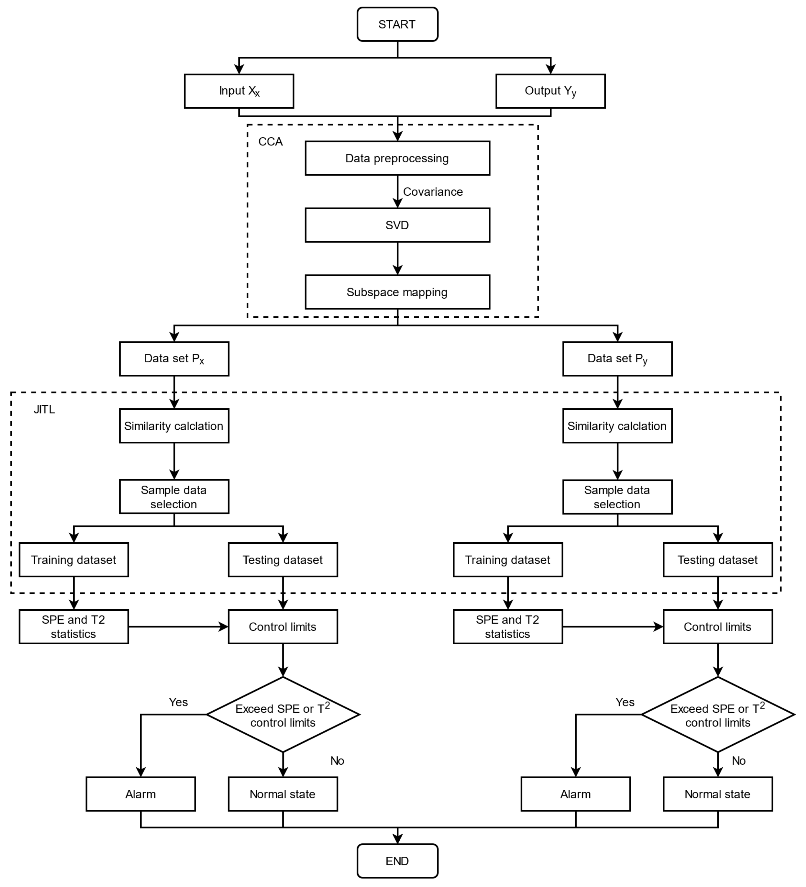
In order to solve the above problems, this paper proposed an FD method based on CCA and JITL. We mainly used the CCA component to preprocess and normalize data, transform high-dimensional data into low-dimensional variable covariance subspaces and maximize the correlation between the most important top latent dimensions. SVD was applied to decompose the covariance matrix of input and output into two separate singular subspaces and keep the original distribution trends of variable correlations. Subspace mapping procedures projects input and output matrices back to the singular subspaces only with the most important relations and generates two groups of variables, Px and Py, after dimension reduction which eliminates the noise, that is, the residual subspaces. Then, JITL was used to calculate the Euclidean similarity of the query sample and the training data, respectively, and selected a sample subset for online testing regarding distances between them. During the experiments, the data sets of Px and Py were equally divided as a training data set and a testing data set. Finally, the FD model formulated statistics to define thresholds of fault signals and performed to detect signal faults in the testing samples. The workflows of the model are shown in Figure 2.

3. Methodology

In this section, combined with the characteristics of signals of the running gears, CCA-JITL FD model is introduced in details.

3.1. Canonical Correlation Analysis and Just-in-Time Learning Methods

CCA transforms covariance matrices of input and output datasets into two subspaces with the greatest correlation by computing the linear combination of the latent dimensions. The algorithm is adopted by using singular value decomposition (SVD), and it can preserve the original trend of the data [4,32]. The algorithm maximizes Pearson coherence between $X_x$ and $Y_y$. Pearson correlation of data sets $X_x$ and $Y_y$ can be expressed as [4]

$$R\left(X_{\mathrm{x}},Y_{\mathrm{y}}\right)=max\frac{u^T{S}_{XY}v}{\sqrt{u^T{S}_{XX}u}\sqrt{v^T{S}_{YY}v}}$$

(4)

where $S_{XY}=X_x^T{Y}_y$, $S_{XX}=X_x^T{X}_x$ and $S_{YY}=Y_y^T{Y}_y$. According to the data set $X_x$ and $Y_y$ given above, standardization is carried out, respectively. Calculation of matrix is [6]

$$W=S_{XX}^{-\frac{1}{2}}{S}_{XY}{S}_{YY}^{-\frac{1}{2}}=\frac{X_x^T{Y}_y}{\sqrt{X_x^T{X}_x}\sqrt{Y_y^T{Y}_y}}$$

(5)

The matrix W is decomposed by singular value decomposition (SVD), and the W is decomposed as [4]

$$\mathrm{W}=\mathsf{\Gamma }D{V}^T$$

(6)

where $\mathsf{\Gamma }=\left(u_1,\dots ,u_{\mathrm{t}}\right)$, $D=\left[\begin{array}{cc}{D}_h& 0\\ 0& 0\end{array}\right]$, $V=\left(v_1,\dots ,v_n\right)$, and where h represents the number of top-ranking singular values and ${\sum }_h=diag\left({\rho }_1,\dots ,{\rho }_h\right)$. Through the formula $\omega =\mathsf{\Gamma }(:,1:h),\psi =V(:,1:h)$, the related subspaces $H_x$ and $H_y$ are generated as [6]

$$\begin{array}{cc}\hfill & H_x=S_{XX}^{-\frac{1}{2}}\omega =\frac{1}{\sqrt{X_x^T{X}_x}}\omega \hfill \\ \hfill & H_y=S_{YY}^{-\frac{1}{2}}\psi =\frac{1}{\sqrt{Y_y^T{Y}_y}}\psi \hfill \end{array}$$

(7)

The latent space of $X_x$ is divided into two subspaces, namely the related subspaces with $Y_y$ and the unrelated subspaces with $Y_y$. Similarly, the latent space of $Y_y$ is divided into two parts, namely the related subspaces with $X_x$ and the unrelated subspaces with $X_x$. According to the above parameters, the original data inputs are mapped to the related latent spaces, $H_x$ and $H_y$, and obtain two associated matrices, $P_x$ and $P_y$. The correlation coefficient is $\rho 1$ between $H_x$ and $H_y$ if only considering the first canonical variate pair of CCA. The data matrix can be formulated as

$$\begin{array}{cc}\hfill & P_x=u=H_x{\left(X_x{\left(H_x^T{H}_x\right)}^{-1}{H}_x^T\right)}^T\hfill \\ \hfill & P_Y=v=H_y{\left(Y_y{\left(H_y^T{H}_y\right)}^{-1}{H}_y^T\right)}^T\hfill \end{array}$$

(8)

The following JITL algorithm is carried out on $P_x$ and $P_y$, respectively, for data fitting. Different from the traditional global model approach, this JITL-based approach uses an online local model structure which could effectively track the current status of the algorithm.

JITL is to improve the prediction of the local FD model using similarity measures. After the most relevant normal data selected from the database, the distance measure, e.g., Euclidean distance $d\left(t_s^{\prime },t_c\right)={∥t_s^{\prime },t_c∥}_2$, is employed to evaluate the similarity between $t_s^{\prime }$ and $t_c$. Here, $t_s^{\prime }$ is the data point of the training set, $t_c$ is the data point of the test set; that is, a smaller value of distance implies a greater similarity between these two vectors [26]. The inverse of Euclidean distance is used to find the correlation between two vectors.

$$S_{i,k}=\frac{1}{\sqrt{e^{{\left({∥t_s^{\prime },t_c∥}_2\right)}^2}}},i = 1,2,3,\dots ,N$$

(9)

where $S_{i,k}$ represents the magnitude of correlation.

Remark 3.

The JITL algorithm arranges $S_{i,k}$ values in descending order. The number of data to be selected is determined by calculating the accumulated contribution value of $S_{i,k}$ to the variance of the overall data, and the formula for the average value of $S_{i,k}$ is ${\theta }_i=\left({\sum }_{i=1}^N{S}_{i,k}\right)/N$. The variance formula is $G={\left(S_{i,k}-{\theta }_i\right)}^2$. The contribution parameter G is used to determine how many data points to be included in the testing sample data. For example, the algorithm picks 900 data points until the sum of G value reach $90\%$.

Remark 4.

JITL selects testing data points which have lower correlations with training dataset. In the experiment, the system only takes the last 900 data points from the sorted testing dataset.

3.2. Monitoring Statistics of FD Models

This section describes the test statistics used for FD. This article uses $T^2$ and SPE for FD. Firstly, a data matrix to be detected is given. Let the input and output matrices obtained after the JITL processing be ${\mu }_x=\left[{\alpha }_{\mathrm{r}}\left(1\right),\dots ,{\alpha }_{\mathrm{r}}\left(N\right)\right]\in R^{l\times N}$, ${\mu }_y=\left[{\alpha }_{\mathrm{c}}\left(1\right),\dots ,{\alpha }_{\mathrm{c}}\left(N\right)\right]\in R^{m_{\times N}}$. According to the Formulas (5)–(7), the residual vector is obtained [6]

$$s=H_y^T{\mu }_x-M^T{\mu }_y$$

(10)

where $M^T=D_h{H}_x^T$.

In the FD algorithm, statistics and their corresponding thresholds define the boundaries of system prediction. $T^2$ and SPE are the two most commonly used statistics in FD [33,34,35,36]. Taking the two data matrices $P_x$ and $P_y$ perform separately FD. The detection of the subspaces is the same as the routine detection process. Then, judging whether the input signals normally or not requires the following methods [4]

$$\begin{array}{cc}\hfill & SPE=s^{T}s\hfill \\ \hfill & SP{E}_x\le J_{x,th}\mathrm{and}SP{E}_y\le J_{y,th}\Rightarrow \mathrm{fault}-\mathrm{free}\hfill \\ \hfill & SP{E}_x>J_{x,th}\mathrm{or}SP{E}_y>J_{y,th}\Rightarrow \mathrm{faulty}\hfill \end{array}$$

(11)

where $J_{x,th}$ and $J_{y,th}$ are the thresholds for $SP{E}_x$ and $SP{E}_y$, respectively. Then, judging whether the input signals normally or not need methods as following [4]

$$\begin{array}{cc}\hfill & T^2=s^T{\Lambda }^{-1}s\hfill \\ \hfill & T_x^2\le T_{x,th}\mathrm{and}{T}_y^2\le T_{y,th}\Rightarrow \mathrm{fault}-\mathrm{free}\hfill \\ \hfill & T_x^2>T_{x,th}\mathrm{or}{T}_y^2>T_{y,th}\Rightarrow \mathrm{faulty}\hfill \end{array}$$

(12)

where s is residual matrix, $T_{x,th}$ and $T_{y,th}$ are the thresholds for $T_x^2$ and $T_y^2$, respectively.

3.3. Offline Training and Online Detection Algorithms

The procedures in Algorithm 1 are used for offline training. The steps in Algorithm 2 are used for online detection.

Algorithm 1 Offline training

1: Normalize the measurement data. 2: The data is divided into two data matrices via CCA model. 3: The JITL model is used to improve accuracy of data fitting. 4: Find the thresholds $J_{x,th}$ and $T_{x,th}$ associated with the data matrix $P_x$, and the thresholds  $J_{y,th}$ and $T_{y,th}$ associated with the data matrix $P_y$.

Algorithm 2 Online detection

1: The collected fault data is normalized. 2: Find the two data matrices. 3: The JITL model is used to improve accuracy of data fitting. 4: Calculate SPE and $T^2$ via (11) and (12). 5: Determine whether a fault occurs comparing the test statistic with the thresholds.

3.4. System Evaluation Methodology

To measure the performance of the FD models, the most commonly used evaluation metrics are the false alarm rate (FAR) and fault detection rate (FDR). FAR uses the probability to quantify the occurrence of alarm when there is no fault. FDR uses the probability to quantify the occurrence of the alarm method in the case of actual failure.

According to the threshold calculated above, FARs and FDRs can be expressed as follows

$$FAR=\frac{M_j}{M_{th}}\times 100\%$$

(13)

where $M_j$ is the number of test statistics higher than the threshold in fault-free conditions, $M_{th}$ is the total number of test statistics.

$$FDR=\frac{B_j}{B_{th}}\times 100\%$$

(14)

where $B_j$ is the number of test statistics higher than the threshold after injection of fault, and $B_{th}$ is the total number of test statistics after fault injection.

Receiver Operating Characteristic (ROC) curves represent the performance of the model at different thresholds. The X axis of the curve is the false positive rate, and the Y axis is the true positive rate. The ideal is an inverted L-shaped curve [37]. The calculation formulas of the true positive rate (TPR) and false positive rate (FPR) are [38]

$$\begin{array}{cc}\hfill & TPR=\frac{TP}{TP+FN}\hfill \\ \hfill & FPR=\frac{FP}{TN+FP}\hfill \end{array}$$

(15)

where $TN$ is actually the number of samples classified into negative samples, $FP$ is actually the number of samples classified into positive samples, $FN$ is actually the number of samples classified into negative samples, $TP$ is actually the number of samples classified into positive samples.

The Area Under a ROC Curve (AUC) is a comprehensive measure of sensitivity and specificity across all possible threshold ranges. It represents the probability that a classifier will rank randomly selected positive instances higher than randomly selected negative instances. The AUC ranges from 0 to 1. The closer AUC is to 1, the better FD performance [38]. The calculation formula is

$$AUC=\sum _{i=1}^N\frac{\left(TPR\right(i)+TPR(i+1\left)\right)\left(FPR\right(i+1)-FPR(i\left)\right)}{2}$$

(16)

4. Experimental Results and Discussion

High-speed train running gears systems are considered to verify the reliability of the proposed algorithms. When the data of the running gears is chosen, and in order to guarantee the consistency of the experiment input, signal data of the running parts was adopted from the same train and the same carriage. In order to guarantee the validity of the data, the monitoring data at the speed of 1000 r/min or above were utilized in the model. The paper uses real data of a running gears system with fault signals to simulate the settings of the experiments very close to the real situations.

4.1. Experimental Verification

Figure 3 shows two correlated subspaces of the input dataset. Figure 3a shows each input variable in the data set $P_x$. The charts of variables from top to bottom belong to bogie 1, bogie 2, motor-driven side bearing, and non-driven side bearing, respectively. Figure 3b shows each variable in the data set $P_y$. From top to bottom, the charts represent motor side big gear, wheel side pinion, wheel side motor big gear, and motor side pinion, respectively.

• Fault Injection: Under the given speed 1000 r/min of high-speed trains, 1000 × 8 samples under health and fault conditions are collected from eight sensors as data sets. Fault data was injected from the 500th data points of the sample test dataset.
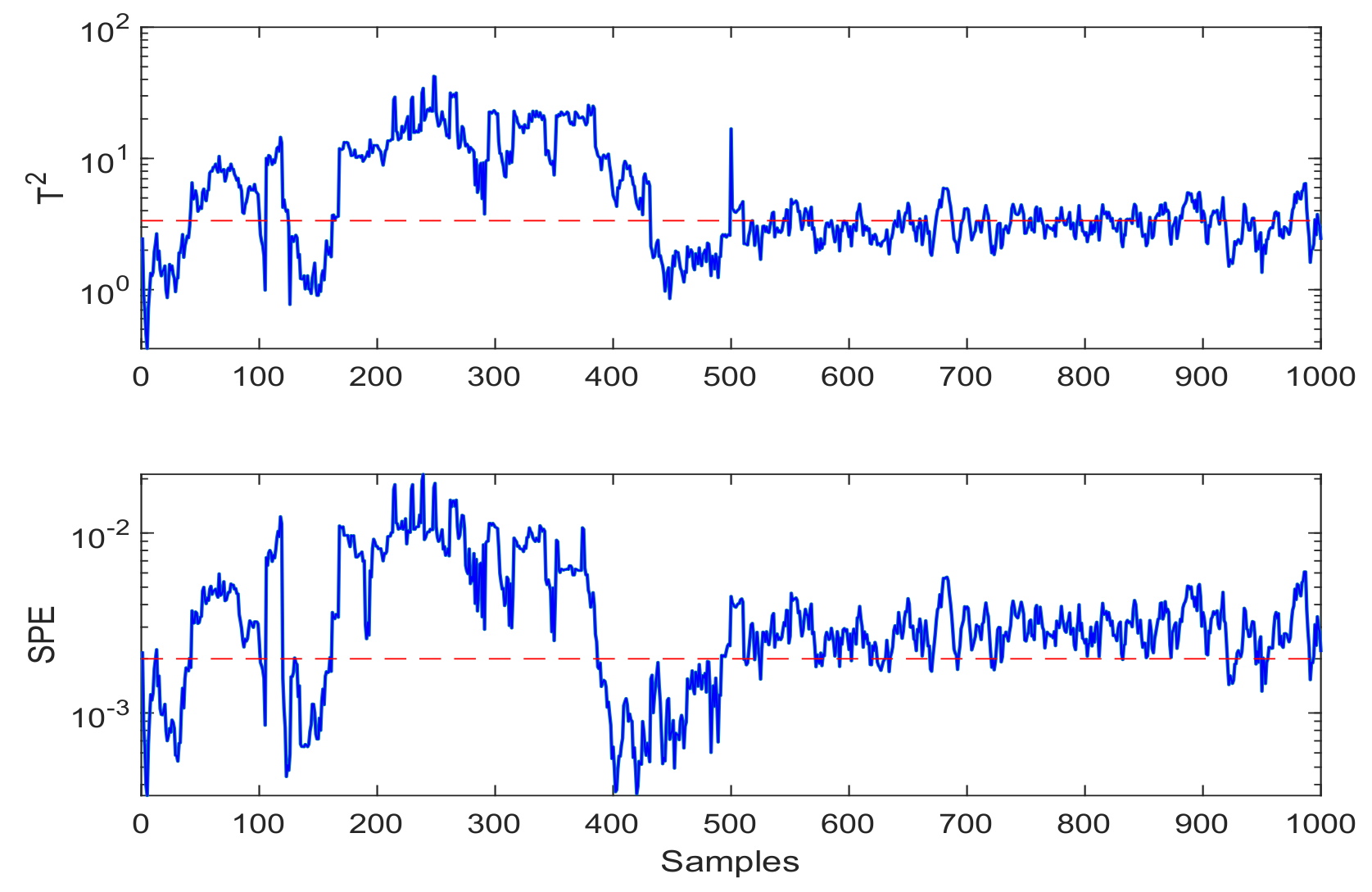
• Fault Detection: Fault detection results of CCA-JITL are shown in Figure 4 where red dashed lines are thresholds and blue sold lines are test statistics.

4.2. Discussions

In order to prove the reliability of the method in this paper, several points will be discussed: (1) the problem solved by this method; (2) the comparison analysis based on the FAR and FDR; (3) the feasibility of the proposed algorithms is testified.

CCA-JITL FD model was applied to detect fault signals of the running gears in two groups in which the results were compared to each other to improve detection accuracy. The method uses CCA to group data and a JITL algorithm to optimize selection of sample data points, so as to achieve better FD performance based on the data shown in Figure 4. Figure 4a depicts the CCA-JITL FD output based on data set $P_x$, and Figure 4b is the result of CCA-JITL FD based on data set $P_y$. The number of singular vectors, h values, decide the proximity of dimension reduction and affect FAR and FDR very much. We tuned parameters and concluded that when $h=2$, CCA-JITL models achieved the best performance.

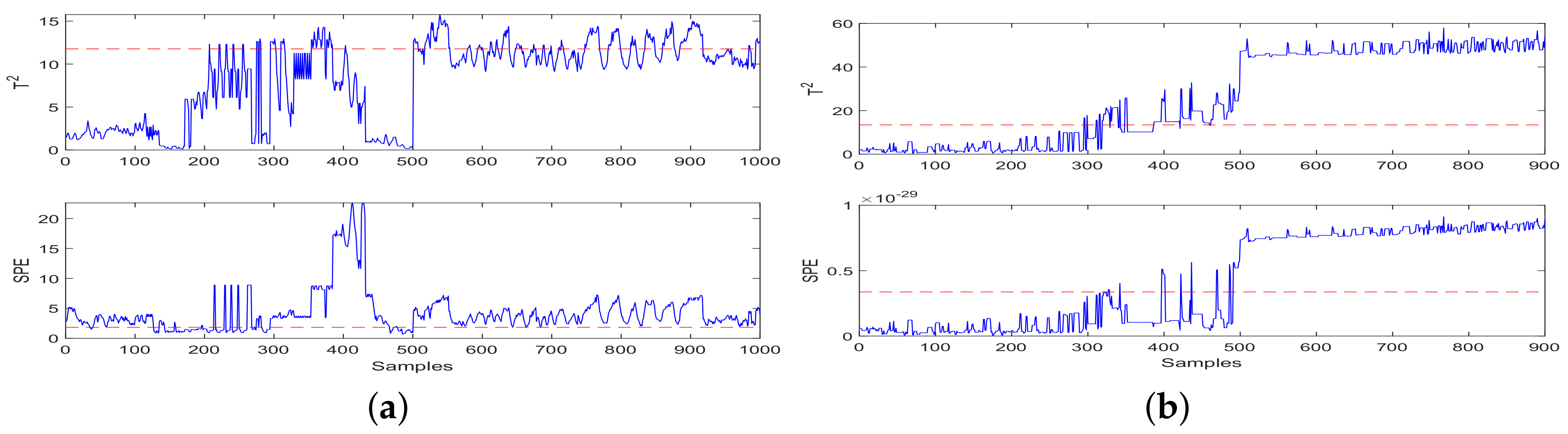
Figure 5 shows FD experiment results using only CCA. The system infrastructure of CCA-JITL was generalized to be utilized to other FD models using PCA and PLS. FD experiment results using SVD-based PLS and JITL are shown in Figure 6. FD experiment results using PCA and JITL are shown in Figure 7. FD experiment results using only PCA are shown in Figure 7.

Based on the detection results shown in Figure 4, the detection of data set $P_x$ after injection fault data is normal, and the detection results of data set $P_y$ show short-term and transient fluctuations after fault injection. Then, the statistics fall back above the threshold. The detection results of the datasets $P_x$ and $P_y$ are compared with each other to verify the performance after injecting fault data, Figure 4a detects a fault, and Figure 4b shows short-term fluctuations. Then, the statistics fall back above the threshold. According to the comparison and verification of the FD results, it was proved that the fault detection at the 500th sample was accurate. Based on the detection results shown in Figure 5, it was observed that statistics were above the threshold before the injection failure time, so false positives have occurred. Moreover, after the injection fault, there is a fluctuation of the statistical value lower than the threshold value, and there is a situation of false negatives. Based on the detection results shown in Figure 6, in Figure 6a it was observed that statistics were above the threshold before the injection failure time, so false positives have occurred. Additionally, after the injection fault, there is a fluctuation of the statistical value lower than the threshold value, and there is a situation of false negatives. Based on the detection results shown in Figure 6b, detection after fault injection is normal, but the fluctuation of statistical value before injecting fault data was partly above the threshold, so a false positive situation had occurred.

Based on the detection results shown in Figure 7. Based on the detection results shown in Figure 7a. $T^2$ statistics showed a few statistical fluctuations higher than the threshold before the fault injection, so false positive situations have occurred. SPE statistics fluctuated a few times above the threshold before the injection of failure signals and kept below the threshold many times after the fault injection. There are serious false positives and omissions. In Figure 7b it was observed that the short-term or instantaneous fluctuations of $T^2$ scores were above the threshold before the fault injection time, so false positive situations had occurred. In the detection results of this method, SPE statistics fluctuation indicates that the SPE scores fluctuate higher than the thresholds before a fault signal is added and then if the SPE scores remain below the threshold, thus, false negative situations have occurred.

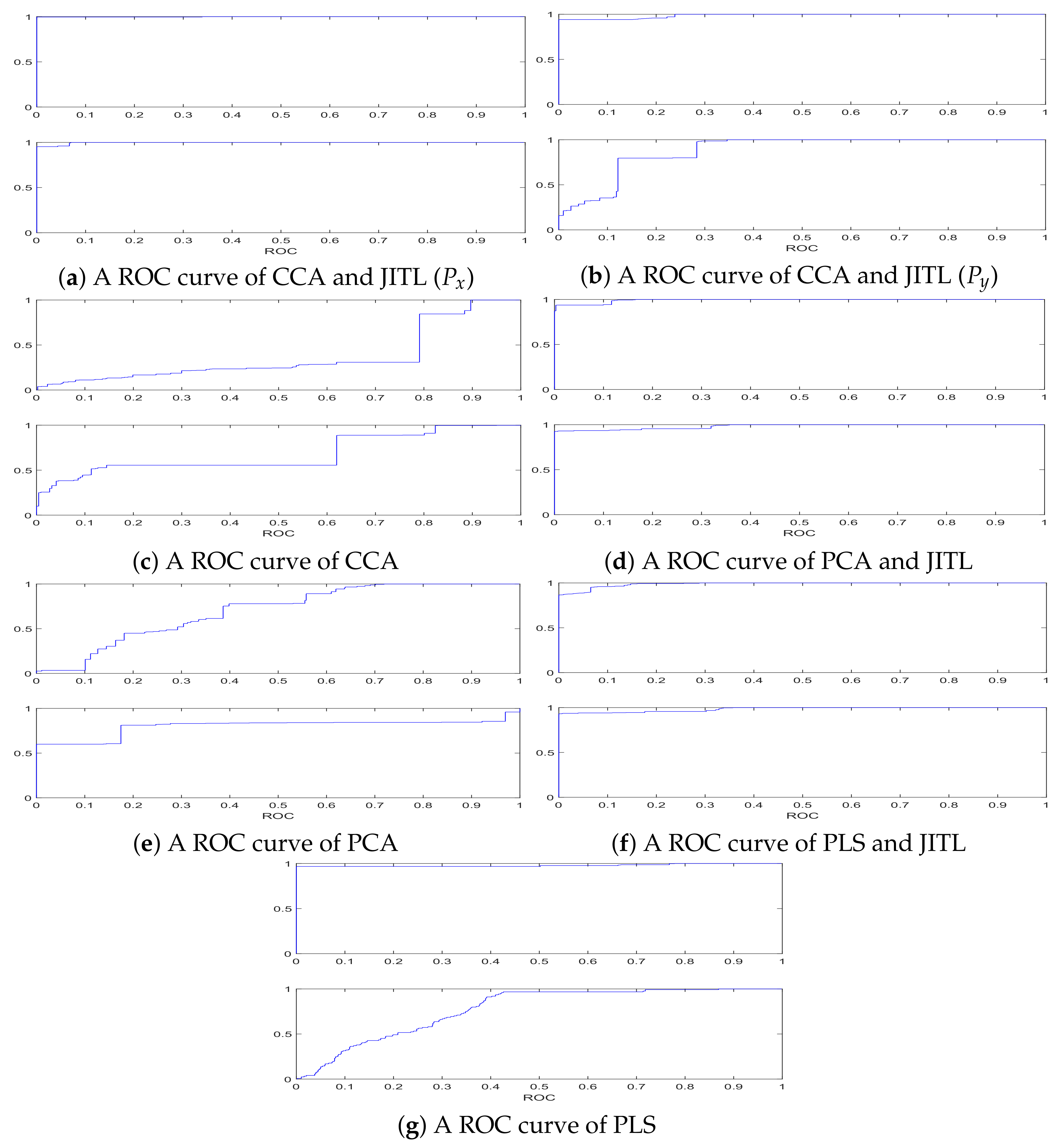
As shown in Figure 8, the receiver operating characteristic (ROC) curves of CCA-JITL, CCA, PLS-JITL, PLS, PCA-JITL and PCA are compared. The ROC curves of each method from top to bottom represent the ROC curves of the model when $T^2$ statistics and SPE statistics are used, respectively. Combined with the area under the curve (AUC) the score of each method shown in

Table 1. Online Testing Results of FD models.

Methods	FAR		FDR		AUC
	${\mathit{T}}^2$	SPE	${\mathit{T}}^2$	SPE	${\mathit{T}}^2$	SPE
PLS	8.81%	45.69%	100%	17.61%	0.9802	0.7729
PLS and JITL	44.75%	0%	100%	82%	0.8430	0.9261
PCA	14.75%	83.5%	41.6%	100%	0.5612	0.7708
PCA and JITL	28.26%	7.41%	100%	100%	0.9887	0.9798
CCA	69.8%	62.2%	38%	90%	0.3601	0.6775
CCA and JITL ($P_x$)	2.5%	6.5%	100%	100%	0.9961	0.9943
CCA and JITL ($P_y$)	7.75%	29.5%	100%	92.2%	0.9847	0.8778
CCA and JITL (average value)	5.125%	18%	100%	96.1%	0.9904	0.9361

. It proved that the performance of CCA-JITL is better than other methods. The AUC values of CCA-JITL, PLS-JITL and PCA-JITL were mostly higher compared with those of PCA, CCA and PLS. The AUC scores of the models increases after adding JITL.

Comparisons of FAR and FDR measures on FD models using CCA-JITL, CCA, PLS-JITL, PLS, PCA-JITL and PCA are shown in Table 1. By comparing FAR and FDR among all algorithms, CCA-JITL worked best for online testing. FAR and FDR scores were calculated regarding $T^2$ and SPE statistics, respectively. The average scores of FAR and FDR were considered to be used in the result comparison. Compared with the CCA method, the average FAR score of CCA-JITL was reduced by $54.44\%$ across both $T^2$ and SPE measures, and the average FDR score was increased by $34.05\%$. Compared with algorithms based on PCA-JITL or PLS-JITL, the FAR score of CCA-JITL is lower. The JITL component improved all the FDR scores of all the FD models. PLS, PCA, and CCA showed that the FDR score increased by $32.20\%$, $29.2\%$, and $34.05\%$, respectively, after using JITL. Since the variables of the real data used in this paper are not independent, CCA-JITL method are more favorable for FD of the data in the running gears. The feasibility of the proposed algorithms were testified by the above comparative experiments. JITL is also useful to shape the visual representation of data fitting so that the fault signals were displayed more distinguished.

The model was tested using a new 1000×8 data set as the independent testing set. According to

Table 2. Independent testing of FD models.

Methods	FAR		FDR		AUC
	${\mathit{T}}^2$	SPE	${\mathit{T}}^2$	SPE	${\mathit{T}}^2$	SPE
PLS	4.6%	0.6%	80%	78%	0.7851	0.7861
PLS and JITL	44.5%	0.5%	100%	66.8%	0.9384	0.8506
PCA	13%	66.8%	76.4%	79.6%	0.7370	0.3738
PCA and JITL	0%	2.75%	98.6%	98.2%	0.9975	0.9868
CCA	83.2%	54.2%	16.2%	62%	0.2158	0.7730
CCA and JITL ($P_x$)	13.25%	19%	100%	100%	0.9587	0.9874
CCA and JITL ($P_y$)	34.25%	67.5%	99%	100%	0.8081	0.8291
CCA and JITL (average value)	23.75%	43.25%	99.5%	100%	0.8834	0.9083

, compared with the CCA model, the results of independent testing of the CCA-JITL FD model showed that the AUC score increased, FAR decreased by $33.2\%$, and FDR increased by $60.65\%$. It proved that this approach is generalizable and still had good performance when random new data was applied.

5. Conclusions and Future Studies

In this study, the proposed algorithms have demonstrated significant advantages on the fault detectability in the running gear systems. This paper presents an FD algorithm based on CCA and JITL. After data preprocessing and normalization, CCA transforms high-dimension historical input data matrices from the database into low-dimension subspaces to maximize correlations between the most important latent dimensions. Then, online input sample data is mapped to these subspaces with coordinates. Finally, JITL components measure Euclidean similarity between query samples and historical samples in subspaces and search subsets of query sample data points with largest distance to training data to build local fault detection models. The evaluation results of the case study showed CCA-JITL outperformed traditional CCA very much in terms of FAR and FDR. This approach was also applied to the FD models based on PCA and PLS and achieved better outcomes, which suggested our system infrastructure was transferable to PCA and PLS FD models.

In future, there are still many research directions that are worth further study. The evaluation results in Table 1 and Table 2 suggested that PCA, PLS and CCA FD models have their unique strengths using different evaluation methods, and thus, the study of model fusion strategies will be promising. Moreover, only FD was investigated in this paper, without classifying and diagnosing positions and categories of faults. Different types of FDD machine learning models will be meaningful to detect specific failure points. Another possible direction for optimization is to change the fitting methods of JITL, such as clustering, and the derivation method of CCA, such as Kernel-based CCA, to enhance the performance of the systems. The third possibility is to improve the scope of the model, that is, how to apply the models to dynamic systems. Furthermore, the research investigation on how to support multi-sensor data acquisition will be very useful, for instance, the data acquisition system using FUSED deposition modeling [39]. Moreover, the method of using prior prediction to detect the remaining useful life is also an important research direction. These research topics will be considered in order to successfully implement and deliver real-world FDD applications for high-speed train running gear systems of high-speed trains.

References

- Chen, H.; Jiang, B. A Review of Fault Detection and Diagnosis for the Traction System in High-Speed Trains. IEEE Trans. Intell. Transp. Syst. 2020, 21, 450–465. [Google Scholar] [CrossRef]
- Gao, S.; Hou, Y.; Dong, H.; Stichel, S.; Ning, B. High-speed trains automatic operation with protection constraints: A resilient nonlinear gain-based feedback control approach. IEEE/CAA J. Autom. Sin. 2019, 6, 992–999. [Google Scholar] [CrossRef]
- Chen, L.; Hu, X.; Tian, W.; Wang, H.; Cao, D.; Wang, F.Y. Parallel planning: A new motion planning framework for autonomous driving. IEEE/CAA J. Autom. Sin. 2019, 6, 236–246. [Google Scholar] [CrossRef]
- Chen, H.; Jiang, B.; Ding, S.X.; Huang, B. Data-Driven Fault Diagnosis for Traction Systems in High-Speed Trains: A Survey, Challenges, and Perspectives. IEEE Trans. Intell. Transp. Syst. 2022, 23, 1700–1716. [Google Scholar] [CrossRef]
- Ran, G.; Liu, J.; Li, C.; Lam, H.K.; Li, D.; Chen, H. Fuzzy-Model-Based Asynchronous Fault Detection for Markov Jump Systems with Partially Unknown Transition Probabilities: An Adaptive Event-Triggered Approach. IEEE Trans. Fuzzy Syst. 2022, 1. [Google Scholar] [CrossRef]
- Chen, H.; Chen, Z.; Chai, Z.; Jiang, B.; Huang, B. A Single-Side Neural Network-Aided Canonical Correlation Analysis With Applications to Fault Diagnosis. IEEE Trans. Cybern. 2021, 1–13. [Google Scholar] [CrossRef]
- Raveendran, R.; Kodamana, H.; Huang, B. Process monitoring using a generalized probabilistic linear latent variable model. Automatica 2018, 96, 73–83. [Google Scholar] [CrossRef]
- Ge, Z.; Song, Z.; Ding, S.X.; Huang, B. Data Mining and Analytics in the Process Industry: The Role of Machine Learning. IEEE Access 2017, 5, 20590–20616. [Google Scholar] [CrossRef]
- Li, X.; Yang, Y.; Pan, H.; Cheng, J.; Cheng, J. A novel deep stacking least squares support vector machine for rolling bearing fault diagnosis. Comput. Ind. 2019, 110, 36–47. [Google Scholar] [CrossRef]
- Zhu, Q.; Qin, S.J. Supervised Diagnosis of Quality and Process Faults with Canonical Correlation Analysis. Ind. Eng. Chem. Res. 2019, 58, 11213–11223. [Google Scholar] [CrossRef]
- Jiang, Q.; Yan, X. Learning Deep Correlated Representations for Nonlinear Process Monitoring. IEEE Trans. Ind. Inform. 2019, 15, 6200–6209. [Google Scholar] [CrossRef]
- Chen, Z.; Ding, S.X.; Peng, T.; Yang, C.; Gui, W. Fault Detection for Non-Gaussian Processes Using Generalized Canonical Correlation Analysis and Randomized Algorithms. IEEE Trans. Ind. Electron. 2018, 65, 1559–1567. [Google Scholar] [CrossRef]
- Peng, X.; Ding, S.X.; Du, W.; Zhong, W.; Qian, F. Distributed process monitoring based on canonical correlation analysis with partly-connected topology. Control Eng. Pract. 2020, 101, 104500. [Google Scholar] [CrossRef]
- Chen, H.; Li, L.; Shang, C.; Huang, B. Fault Detection for Nonlinear Dynamic Systems With Consideration of Modeling Errors: A Data-Driven Approach. IEEE Trans. Cybern. 2022, 1–11. [Google Scholar] [CrossRef]
- Garramiola, F.; Poza, J.; Madina, P.; del Olmo, J.; Ugalde, G. A Hybrid Sensor Fault Diagnosis for Maintenance in Railway Traction Drives. Sensors 2020, 20, 962. [Google Scholar] [CrossRef] [Green Version]
- Kou, L.; Qin, Y.; Zhao, X.; Chen, X. A Multi-Dimension End-to-End CNN Model for Rotating Devices Fault Diagnosis on High-Speed Train Bogie. IEEE Trans. Veh. Technol. 2020, 69, 2513–2524. [Google Scholar] [CrossRef]
- Zhao, R.; Yan, R.; Chen, Z.; Mao, K.; Wang, P.; Gao, R.X. Deep learning and its applications to machine health monitoring. Mech. Syst. Signal Process. 2019, 115, 213–237. [Google Scholar] [CrossRef]
- Niu, G.; Xiong, L.; Qin, X.; Pecht, M. Fault detection isolation and diagnosis of multi-axle speed sensors for high-speed trains. Mech. Syst. Signal Process. 2019, 131, 183–198. [Google Scholar] [CrossRef]
- Fu, Y.; Huang, D.; Qin, N.; Liang, K.; Yang, Y. High-Speed Railway Bogie Fault Diagnosis Using LSTM Neural Network. In Proceedings of the 2018 37th Chinese Control Conference (CCC), Wuhan, China, 25–27 July 2018; pp. 5848–5852. [Google Scholar] [CrossRef]
- Cheng, C.; Guo, Y.; Wang, J.h.; Chen, H.; Shao, J. A Unified BRB-based Framework for Real-Time Health Status Prediction in High-Speed Trains. IEEE Trans. Veh. Technol. 2022, 1. [Google Scholar] [CrossRef]
- Guan, S.; Huang, D.; Guo, S.; Zhao, L.; Chen, H. An Improved Fault Diagnosis Approach Using LSSVM for Complex Industrial Systems. Machines 2022, 10, 443. [Google Scholar] [CrossRef]
- Sayyad, S.; Kumar, S.; Bongale, A.; Kamat, P.; Patil, S.; Kotecha, K. Data-Driven Remaining Useful Life Estimation for Milling Process: Sensors, Algorithms, Datasets, and Future Directions. IEEE Access 2021, 9, 110255–110286. [Google Scholar] [CrossRef]
- Capriglione, D.; Carratù, M.; Pietrosanto, A.; Sommella, P. Online Fault Detection of Rear Stroke Suspension Sensor in Motorcycle. IEEE Trans. Instrum. Meas. 2019, 68, 1362–1372. [Google Scholar] [CrossRef]
- Shabanian, M.; Montazeri, M. A neuro-fuzzy online fault detection and diagnosis algorithm for nonlinear and dynamic systems. Int. J. Control. Autom. Syst. 2011, 9, 665–670. [Google Scholar] [CrossRef]
- Yan, B.; Yu, F.; Huang, B. Generalization and comparative studies of similarity measures for Just-in-Time modeling. IFAC-PapersOnLine 2019, 52, 760–765. [Google Scholar] [CrossRef]
- Cheng, C.; Chiu, M.S. Nonlinear process monitoring using JITL-PCA. Chemom. Intell. Lab. Syst. 2005, 76, 1–13. [Google Scholar] [CrossRef]
- Bittanti, S.; Picci, G. Identification, Adaptation, Learning: The Science of Learning Models from Data; Springer Science & Business Media: Berlin/Heidelberg, Germany, 1996; Volume 153. [Google Scholar]
- Yu, H.; Yin, S.; Luo, H. Robust Just-in-time Learning Approach and Its Application on Fault Detection. IFAC-PapersOnLine 2017, 50, 15277–15282. [Google Scholar] [CrossRef]
- Chen, H.; Chai, Z.; Jiang, B.; Huang, B. Data-Driven Fault Detection for Dynamic Systems with Performance Degradation: A Unified Transfer Learning Framework. IEEE Trans. Instrum. Meas. 2021, 70, 1–12. [Google Scholar] [CrossRef]
- Ran, G.; Li, C.; Lam, H.K.; Li, D.; Han, C. Event-Based Dissipative Control of Interval Type-2 Fuzzy Markov Jump Systems Under Sensor Saturation and Actuator Nonlinearity. IEEE Trans. Fuzzy Syst. 2022, 30, 714–727. [Google Scholar] [CrossRef]
- Cheng, C.; Qiao, X.; Luo, H.; Teng, W.; Gao, M.; Zhang, B.; Yin, X. A Semi-Quantitative Information Based Fault Diagnosis Method for the Running Gears System of High-Speed Trains. IEEE Access 2019, 7, 38168–38178. [Google Scholar] [CrossRef]
- Cheng, C.; Wang, J.; Teng, W.; Gao, M.; Zhang, B.; Yin, X.; Luo, H. Health Status Prediction Based on Belief Rule Base for High-Speed Train Running Gear System. IEEE Access 2019, 7, 4145–4159. [Google Scholar] [CrossRef]
- Chen, H.; Chai, Z.; Dogru, O.; Jiang, B.; Huang, B. Data-Driven Designs of Fault Detection Systems via Neural Network-Aided Learning. IEEE Trans. Neural Netw. Learn. Syst. 2021, 1–12. [Google Scholar] [CrossRef]
- Kresta, J.V.; Macgregor, J.F.; Marlin, T.E. Multivariate statistical monitoring of process operating performance. Can. J. Chem. Eng. 1991, 69, 35–47. [Google Scholar] [CrossRef]
- Wise, B.M.; Gallagher, N.B. The process chemometrics approach to process monitoring and fault detection. J. Process. Control 1996, 6, 329–348. [Google Scholar] [CrossRef]
- Chiang, L.H.; Russell, E.L.; Braatz, R.D. Fault Detection and Diagnosis in Industrial Systems; Springer Science & Business Media: Berlin/Heidelberg, Germany, 2000. [Google Scholar]
- Kumar, D.; Ding, X.; Du, W.; Cerpa, A. Building sensor fault detection and diagnostic system. In Proceedings of the 8th ACM International Conference on Systems for Energy-Efficient Buildings, Cities, and Transportation, Coimbra, Portugal, 17–18 November 2021; pp. 357–360. [Google Scholar]
- Li, G.; Zheng, Y.; Liu, J.; Zhou, Z.; Xu, C.; Fang, X.; Yao, Q. An improved stacking ensemble learning-based sensor fault detection method for building energy systems using fault-discrimination information. J. Build. Eng. 2021, 43, 102812. [Google Scholar] [CrossRef]
- Kumar, S.; Kolekar, T.; Patil, S.; Bongale, A.; Kotecha, K.; Zaguia, A.; Prakash, C. A Low-Cost Multi-Sensor Data Acquisition System for Fault Detection in Fused Deposition Modelling. Sensors 2022, 22, 517. [Google Scholar] [CrossRef]
Figure 1.
Structure of a running gears system.
Figure 2.
Flowchart of the proposed CCA-JITL FD model.
Figure 3.
The input dataset. (a) Data matrix ; (b) Data matrix .
Figure 4.
Experiment results of CCA-JITL FD model. (a) Data matrix detection; (b) Data matrix detection.
Figure 5.
Experiment results of the FD model using CCA.
Figure 6.
Experiment results of the FD model using PLS. (a) Online testing of the FD model using PLS; (b) Online testing of the FD model using PLS and JITL.
Figure 7.
Experiment results of the FD model using PCA. (a) Online testing of the FD model using PCA; (b) Online testing of the FD model using PCA and JITL.
Figure 8.
The ROC curves of FD models. (a) A ROC curve of CCA and JITL (); (b) A ROC curve of CCA and JITL (); (c) A ROC curve of CCA; (d) A ROC curve of PCA and JITL; (e) A ROC curve of PCA; (f) A ROC curve of PLS and JITL; (g) A ROC curve of PLS.