
The Unsteady-State Response of Tires to Slip Angle and Vertical Load Variations

1
State Key Laboratory of Automotive Simulation and Control, Jilin University, Changchun 130025, China
2
General R&D Institute of China Department Experiment Unit, China FAW Group Co., Ltd., Changchun 130013, China
*
Author to whom correspondence should be addressed.
Machines 2022, 10(7), 527; https://0-doi-org.brum.beds.ac.uk/10.3390/machines10070527
Submission received: 30 May 2022
/
Revised: 25 June 2022
/
Accepted: 27 June 2022
/
Published: 29 June 2022
(This article belongs to the Section Vehicle Engineering)
Abstract
:The tire is the only part that connects the vehicle and the road surface. Many important properties of vehicles are related to the mechanical properties of tires, such as handling stability, braking safety, vertical vibration characteristics, and so on. Although a great deal of research on tire dynamics has been completed, mainly focusing on steady-state tire force and moment characteristics, as well as linear unsteady force characteristics, less research has been conducted on nonlinear unsteady characteristics, especially when the vertical load changes dynamically. Therefore, the main purpose of this paper is to improve the tire unsteady-state model and verify it by experiment. To achieve this goal, we first study the nonlinear unsteady tire cornering theoretical model and obtain clear force and torque frequency response functions. Then, based on the results of the theoretical model, a high-precision and high-efficiency semi-physical model is developed. Finally, model identification and accuracy verification are carried out based on the bench test data. The model developed in this paper has high accuracy, and it significantly improves the expression of the aligning torque, which helps to improve the virtual simulation of transient conditions, such as vehicle handling and dynamic load conditions.
1. Introduction
In recent years, the rapid development of modern technologies, such as computers and controls, has enabled a large number of advanced electronic control technologies to be applied to automobile systems, and various advanced chassis control systems have been continuously developed and applied. The realization of all these chassis control systems is based on the tire force and moment between the tire and the road surface. Therefore, the accurate description of tire mechanical properties is not only the key to the development of advanced chassis control systems but also an important basis for the design, simulation, and evaluation of these control systems [1,2,3,4,5,6,7].
At the same time, with the rapid development of computer technology, advanced vehicle design, simulation, and evaluation technologies, such as virtual prototyping, computer-aided engineering (CAE in short), virtual proving ground (VPG in short), and driving simulator (drive-in-loop), are emerging as the times require, all of which require an in-depth understanding of vehicle dynamics. Therefore, the research on tire mechanical properties also puts forward higher requirements. Numerous studies have shown that tire dynamics have a significant impact on vehicle dynamics [8,9,10,11,12]. How to describe the mechanical properties of tires more accurately and establish a tire mechanical model more in line with engineering needs is an urgent problem to be solved in the research field of automobile dynamics and tire mechanics.
Since the 1930s, research on the mechanical properties of tires has had a history of nearly a hundred years, and a large number of outstanding scholars and experts have emerged to conduct meticulous and in-depth research on the topic [13,14,15,16,17,18,19,20,21]. With the development of electronic computer technology, test equipment, and test technology, tire mechanics has made great progress in theoretical mechanism, virtual simulation, test verification, etc. It basically realizes multi-dimensional tire digital analysis capabilities, including pure mechanical characteristics research in steady-state, transient [22], dynamic [23], and modal aspects, and also covers complex usage scenarios, such as temperature [24,25,26,27], wear, speed, and road conditions, etc. Beregi and Takács have extensively analyzed unsteady dynamics of tires, mainly for the shimmy (turn slip) condition, but research on cornering unsteady force and moment has not been carried out [28,29,30]. Romano et al. have investigated transient effects due to large camber angles and introduced the two-regime transient models that account for nonlinear dynamics connected to combined slip conditions and load variations [31,32,33,34,35,36]. However, the research mainly focuses on the expression of lateral force and longitudinal force, and there are few studies on unsteady aligning torque. These analytical models in the time domain are used for analysis, and the key to guiding practical modeling has not been obtained. Furthermore, the experimental verification is insufficient and needs to be further enhanced.
However, the existing tire unsteady mechanical models are mainly aimed at the simulation of longitudinal force and lateral force under constant load conditions, and there are few studies on high-precision aligning moment characteristics, so the study of tire unsteady force and moment characteristics under dynamic load conditions is still insufficient. Automobiles inevitably drive on various uneven roads. Even on fairly flat roads, vertical vibrations of the wheels are inevitably generated when driving at a high speed, and the vertical load between the tires and the road surface changes sharply. Preliminary tests have been carried out. It is shown that the fluctuation in the vertical load on the tire caused by the fluctuation in the road surface and the change in the motion state of the vehicle has a significant impact on the mechanical properties of the tire, resulting in a large difference in the performance and load analysis of the whole vehicle.
This paper will systematically study the nonlinear dynamic load and unsteady force and moment characteristics of tire sideslip and develop a practical and efficient semi-physical simulation model based on the theoretical model, focus on improving the dynamic load condition model and the non-steady-state aligning moment model, and, finally, conduct a comprehensive indoor bench test verification.
2. Unsteady Cornering Theoretical Model Considering Complex Deformation of Carcass
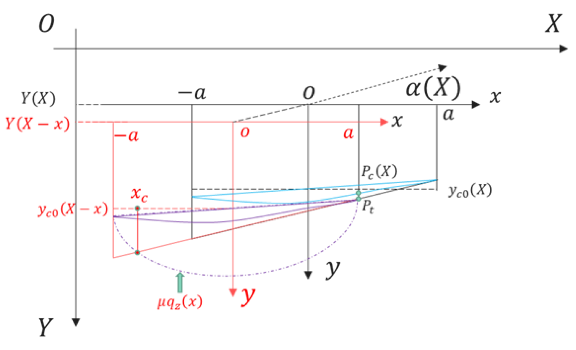
In the previous studies by scholars, a relatively complete unsteady model mechanism in the linear region was basically explored. However, considering that there is still no clear conclusion for the full range of nonlinear theoretical models, in order to better develop semi-physical models of nonlinear non-steady-state (especially the return-to-positive moment model) in the future, we will focus on the non-steady-state nonlinear side deflection theory. As the model is derived, the derivation will be made for the unsteady nonlinear side deflection theoretical model. On the basis of the basic cornering brush model, a complete transient transfer function expression for unsteady nonlinear cornering considering the complex deformation of the carcass is deduced. Specifically, as shown in Figure 1:
The coordinate system establishes the absolute coordinate system of the earth, which is used to describe the overall relative position change of the tire on the road surface; the coordinate system is a relative coordinate system rigidly fixed on the contact patch center (also the contact patch update coordinate system).
The bristles of the tire tread enter from the front end point a of the footprint and leave at -a of the footprint coordinate system after rolling rotation, where a is the half length of the touchdown footprint. Since this section only considers the unsteady motion of the sideslip, the motion input of the model is , which can also be converted into the input of the sideslip angle through its relationship with the longitudinal motion speed.
Modeling assumptions:
- (1)
- The complex deformation (lateral) of the carcass is expressed by the superposition of three deformations of translation, torsion, and bending;
- (2)
- It is used for side deviation analysis without considering the influence of tire width;
- (3)
- For cornering analysis, only the lateral deformation of the tread is considered;
- (4)
- Inertia factors, such as tire mass and gyroscopic effect, are not considered, and it is assumed to be a steady system;
- (5)
- In the initial state (), each state parameter and variable starts from 0 (displacement, deformation, etc.);
- (6)
- For small movements near any slip angle, the slip between the tread end point and the road surface is considered, but the input conditions for small movements of local linearization are still satisfied;
- (7)
- The stiffness and deformation of the tire carcass and tread are not considered;
- (8)
- The pressure distribution of the grounding trace is assumed not to consider the width;
- (9)
- Only pure cornering conditions are considered, and the imprint update speed is consistent with the longitudinal translation speed of the tire;
Figure 1 depicts the tire deformation in two spatial states (or temporal states), expressing the carcass deformation and the tread deformation, respectively. The lower endpoint of the tread unit is when there is no slip in the footprint, and consider that does not move relative to the geodetic fixation. The upper end point of the tread unit is the lower end point of the deformation of the carcass. The deformation of the carcass is expressed as an overall expression of the deformation at different positions in the footprint through the overall deformation distribution function after receiving the lateral force and the aligning moment. First of all, it is pointed out that the lateral position of the tread and the lateral position of the carcass are both bivariate functions of the spatial position in the space domain and the coordinate position in the footprint, and then, according to the assumptions:
The key expressions and principles of the transient model will be introduced below. Since there is no slippage at the ground contact point of the tread, then the tread unit position of the -print position at the -space position (time) can be obtained. In fact, it is also the position where the space position (moment) has just entered the tread bristles, which is:
The lateral coordinate of the carcass is the center position of the rim plus the lateral deformation of the carcass:
The three-direction deformations are:
Define the lateral deformation feature ratio:
The deformation of the carcass is expressed as :
The tread deformation is expressed as :
The road slip velocity is :
It can be seen that the movement direction of is opposite to the deformation direction of the carcass and tread. When the deflection motion input is not considered, the deformation differential equation can be expressed as:
When there is no slip between the tread and the road, , can obtain:
Solution one:
Considering that the deformation of the carcass is a bivariate function of the local coordinate position and the global coordinate position , Equation (15) is deduced:
Further simplification of Equation (16), where is the footprint update speed, is the tire longitudinal movement speed, by defining and , we can obtain:
Considering the pure sideslip condition, there is :
Laplace transform the function with respect to the spatial position :
Quoting the general solution of the inhomogeneous first-order differential equation :
Bring in the boundary conditions (the initial deformation is 0), when , , there are:
Solution two:
This method is based on the principle of accumulated deformation of a certain bristle over a certain period of time. First, the rolling experience time of different imprint positions is determined, and the distance of imprint update in this time is :
Then, for any bristles in the imprint, it is obtained by just entering the imprint (zero deformation) and undergoing time deformation, so the tread deformation should be obtained by integrating the tread deformation speed in time :
Considering the pure cornering condition and does not change within time , there are:
Laplace transform the function with respect to the spatial position
When considering the motion input in the nonlinear region, the slip between the tread and the road surface should be considered, that is, the slip occurs when the lateral stress exceeds the adhesion limit of the road surface (). At this point, the coordinate is in the start-slip point footprint. In the process of solving the lateral force and moment, it should be considered that it is divided into two sections for integration, the attachment area and the slip area, and is used as the dividing boundary.
Sideslip lateral force solution:
To further simplify the solution, assume a small movement around an effective slip angle. That is, can be assumed to be a constant value after a given effective slip angle. The analysis of the frequency characteristics of the transfer function based on local linearization is a response that expresses the input change process and the output change and examines the relationship between the output and the input change gradient.
In the same way, the transformation result of the change amount of the aligning torque is:
Compared with the integration process in the previous section, the nonlinear region analysis mainly changes the lower limit of the integration, so it only affects the expression and solution of the characteristic function. First define the parameter of the parameter start-slip point in the footprint, and then there is:
The solution process of the characteristic functions and is as follows:
The expressions of the transfer functions of the lateral force and the aligning torque are still consistent with the derivation results in the previous section, and only the characteristic functions are replaced:
Through the above derivation, a comprehensive nonlinear sideslip frequency characteristic analysis can be carried out, and it can be seen that the key parameter of the above frequency characteristic is the characteristic parameter of the starting-slip point. In order to more intuitively show the difference in frequency characteristics at different slip-angle positions, the relationship expression between and is introduced. When the carcass is rigid (the same relationship is used for simplification when the carcass is flexible), there is:
Set to be the path frequency (and define dimensionless path frequency for simplified analysis), make , and substituting into the above expression can obtain the frequency characteristics of lateral force and aligning moment corresponding to different sideslip angle positions under tire cornering motion input conditions. The following figures (Figure 2 and Figure 3) show the unsteady frequency characteristic curves without considering the elasticity of the carcass and considering the complex deformation of the carcass:
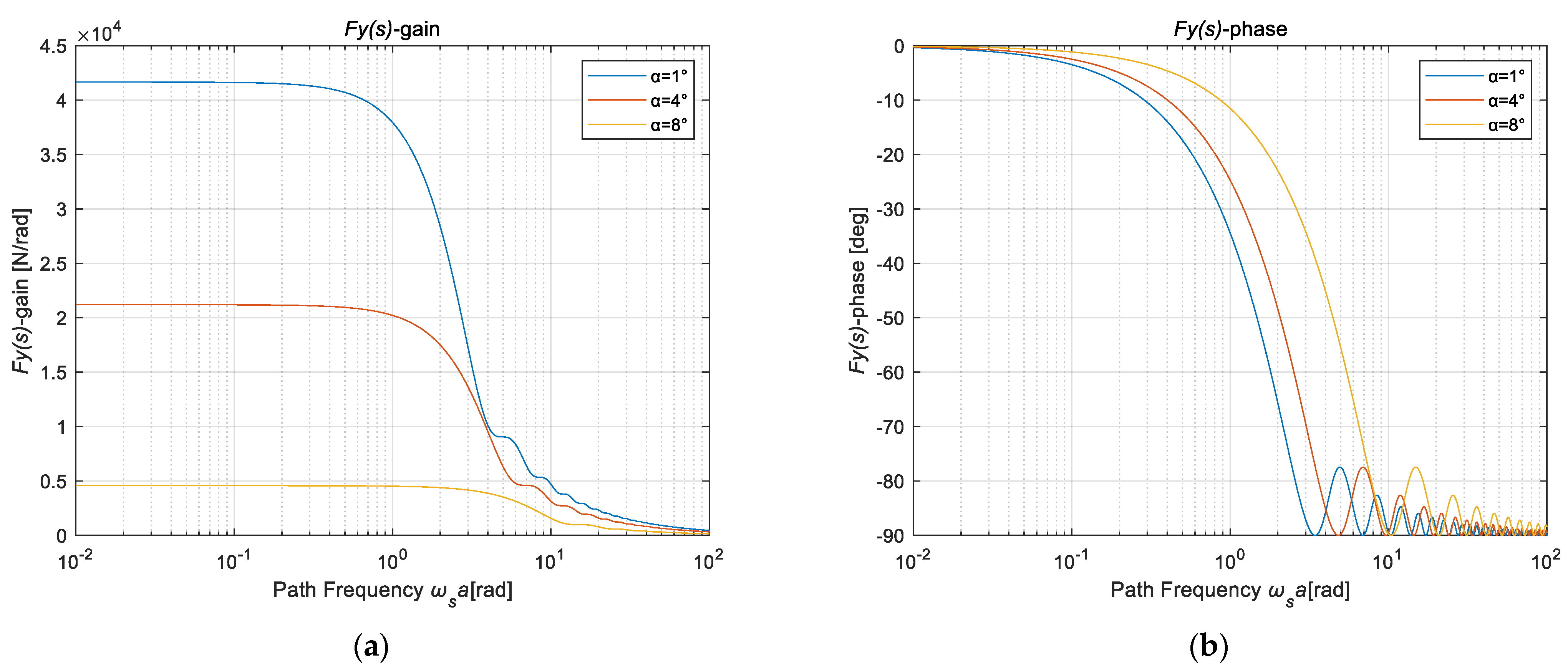
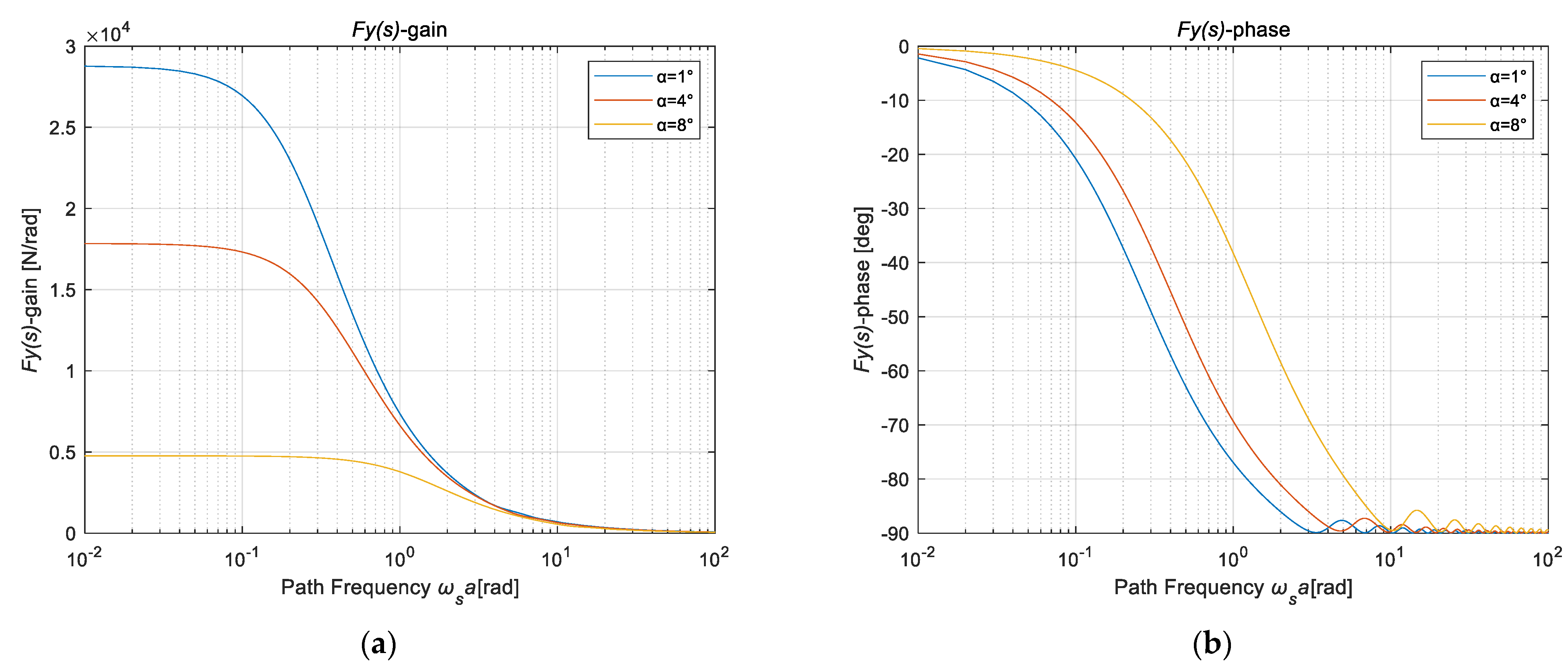
As can be seen from the above figure, when at different slip angle levels, the lateral force response basically satisfies the conditions of first-order behavior. Its steady-state gain is the derivative of the lateral force to the sideslip angle at this point during steady-state sideslip, and it decreases with the increase in the sideslip angle (without considering the dynamic friction), and the cut-off frequency increases with the increase in the sideslip angle. However, the response of the aligning moment shows a more complex phenomenon. In order to analyze the nonlinear frequency characteristics of the lateral force and the aligning moment more clearly, adjust the form of the coordinate axis and set the deflection input near the zero-deflection level. Amplitude–frequency characteristics of lateral force and realigning moment are shown in Figure 4:
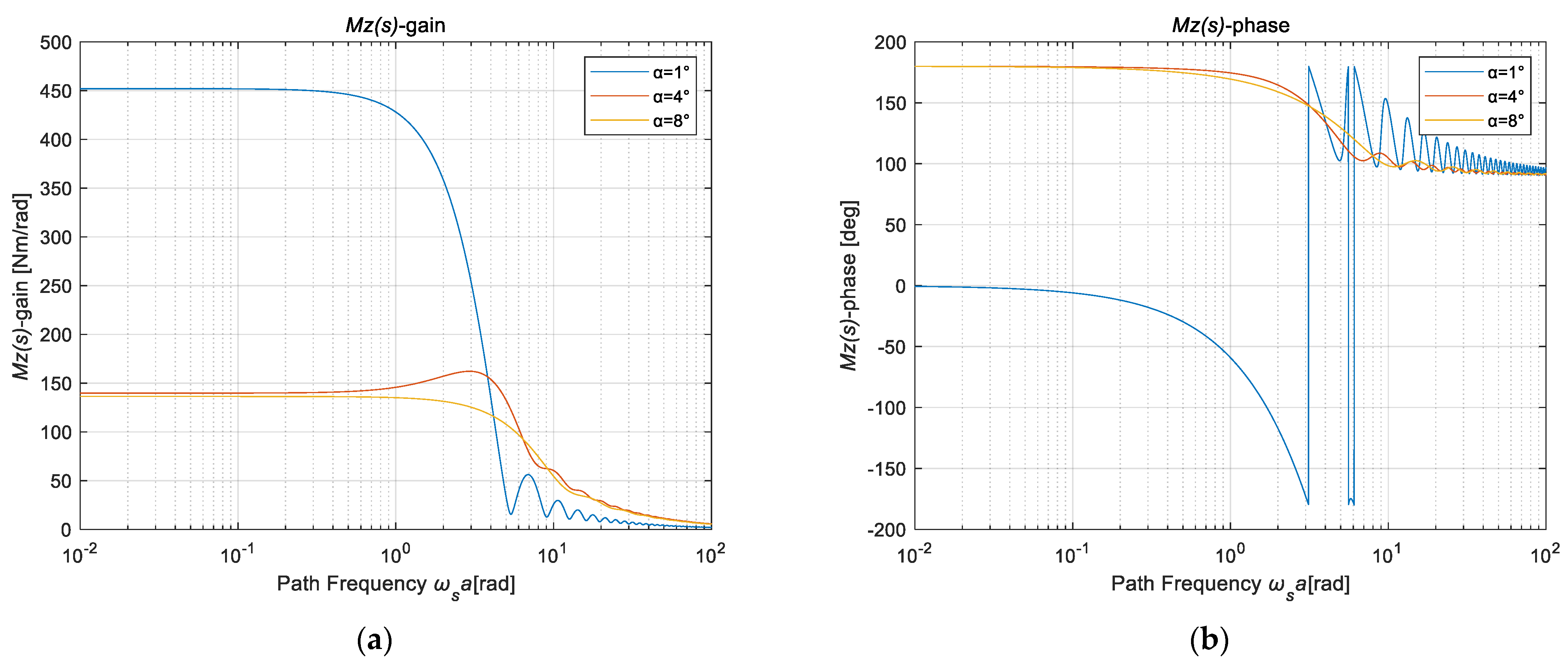
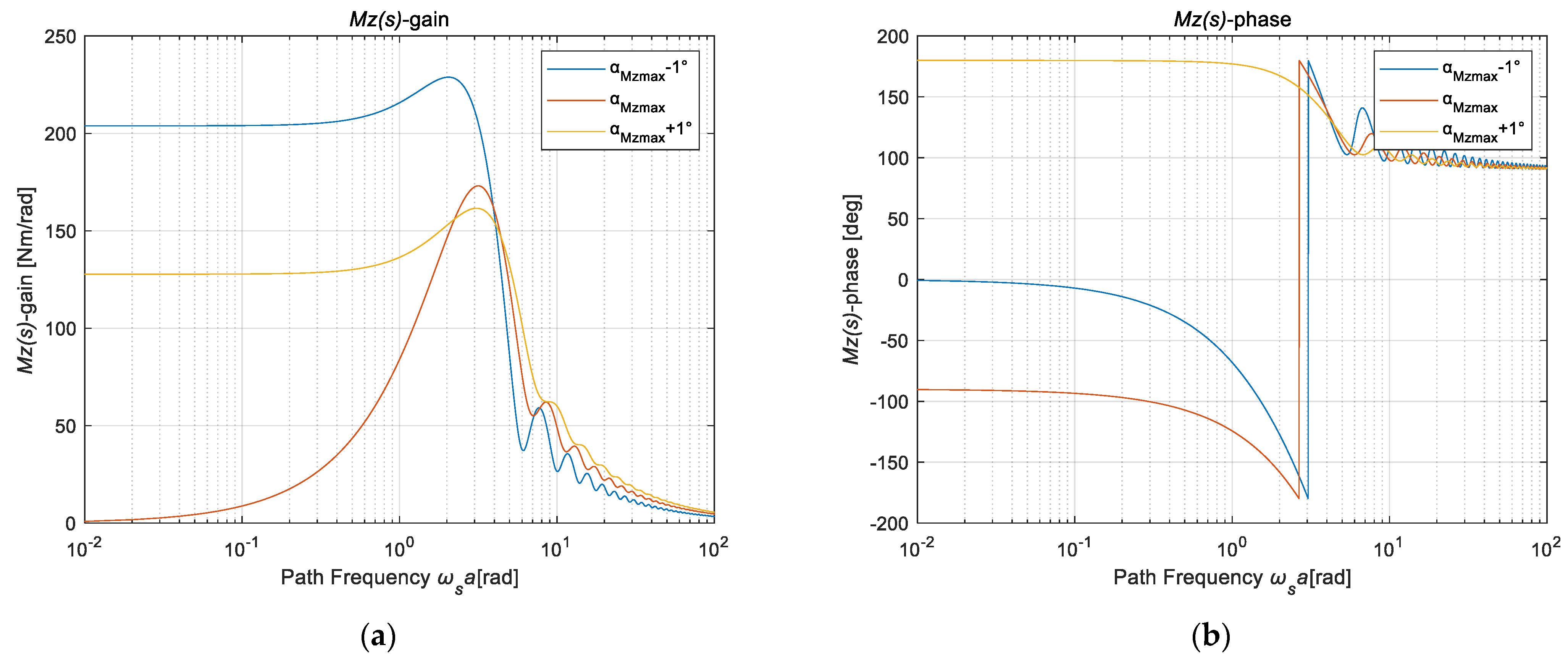
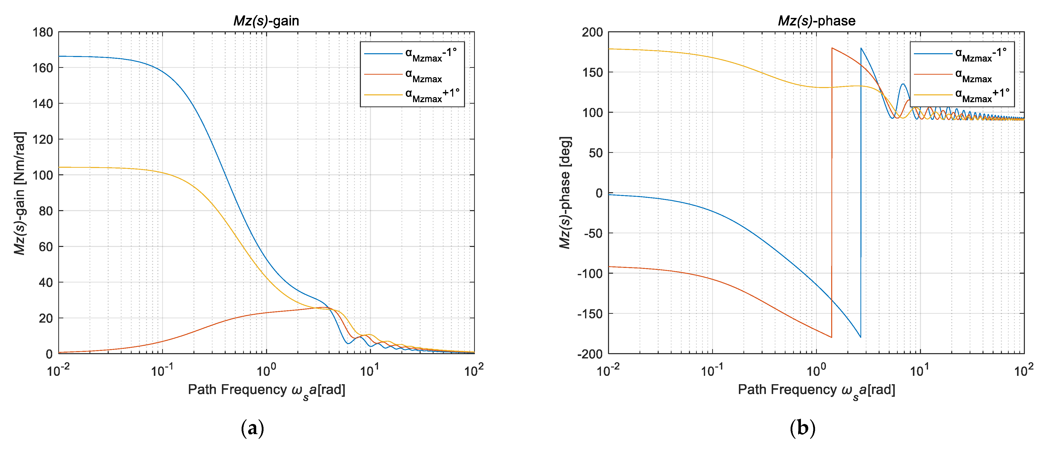
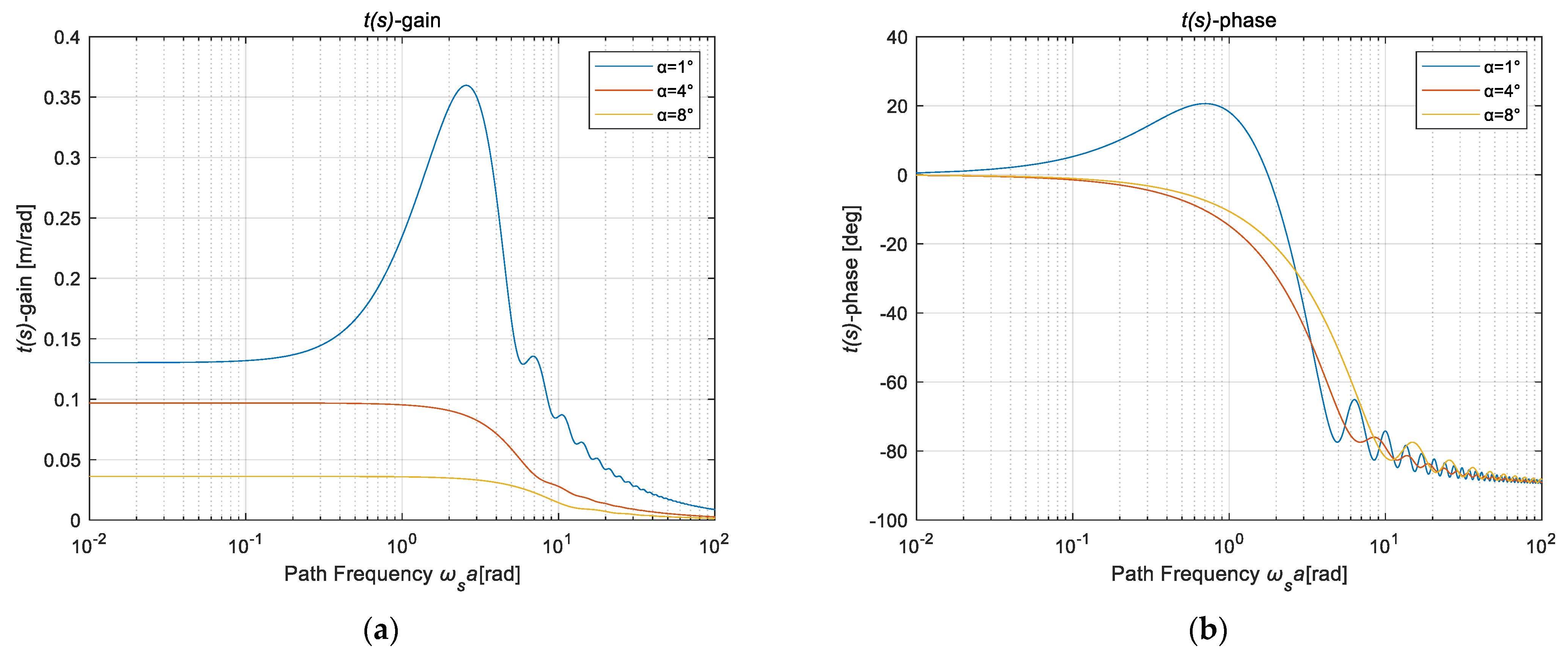
Figure 4 shows that the high-frequency asymptotes of the amplitude of the lateral force are reduced by 20 dB (decreased by ten times) for each additional decade of frequency band under each lateral deviation level, which is a typical first-order behavior. However, the magnitude response of the aligning moment is near zero slip angle, and the high-frequency asymptote is −40 dB per decade, indicating that it is a typical second-order behavior, gradually becoming a first-order behavior. Its steady-state gain is the derivative of the aligning torque to the sideslip angle at this point during steady-state sideslip. Therefore, the sign changes when the slip angle is at the maximum of the aligning torque. This will result in a 180° shift in the initial phase of the aligning torque and an “overshoot” phenomenon (two cutoff frequencies) in the magnitude response around the peak slip angle of the aligning torque. The behavior near the peak is shown in the following figure (Figure 5):
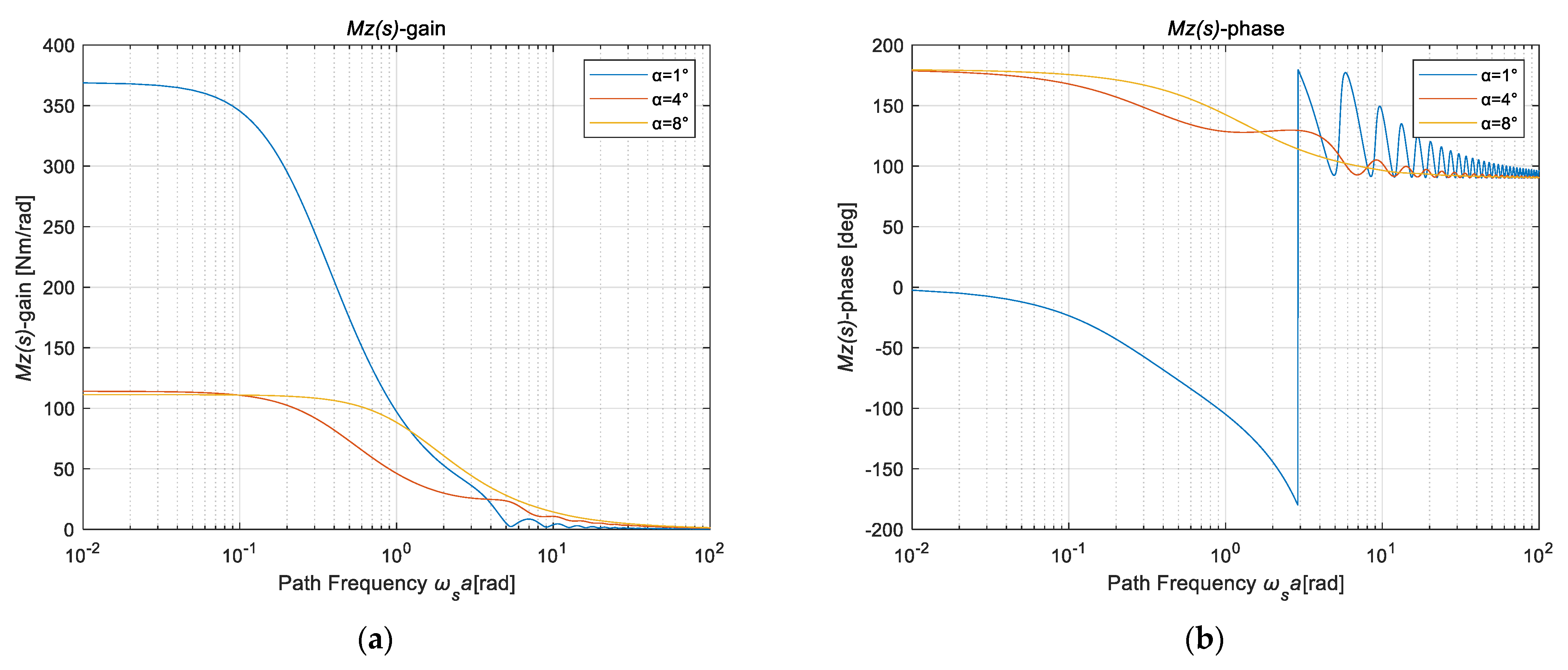
Summary: The frequency characteristics near the peak of the aligning torque show obvious overshoot, and the amplitude response has a typical double cutoff frequency. Although the high-frequency asymptote satisfies the first-order behavior, it is not a simple and typical first-order system. Further in-depth analysis and research need to be carried out in combination with the response of the pneumatic trail. The following figures (Figure 6, Figure 7 and Figure 8) will briefly introduce the frequency response characteristics of lateral force and aligning torque after considering the complex deformation of the carcass:
Conclusion: After considering the complex deformation of the carcass, the frequency response characteristics of the lateral force are still relatively clear, but the response of the aligning torque becomes more complex, and the law described above remains unchanged. Only the degree of characterization and details of the characteristics have changed, so the analysis results described above can be used.
In actual use and research, the aligning torque is usually expressed as the product of the lateral force and the pneumatic trail, where the pneumatic trail represents the distribution of the lateral force in the footprint. Therefore, in order to better study the characteristics of the aligning torque, it is necessary to further analyze and study the frequency characteristics of the pneumatic trail.
Ignore the second-order term and divide into steady-state value and variable fluctuation:
Arranging Equation (44), the expression for the aligning torque can obtain:
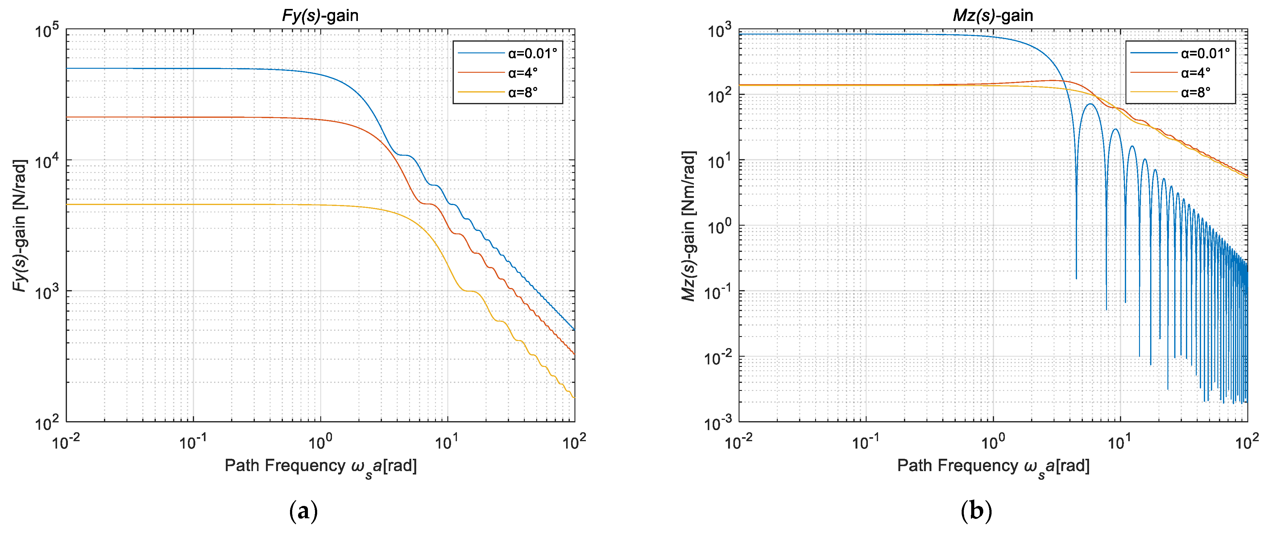
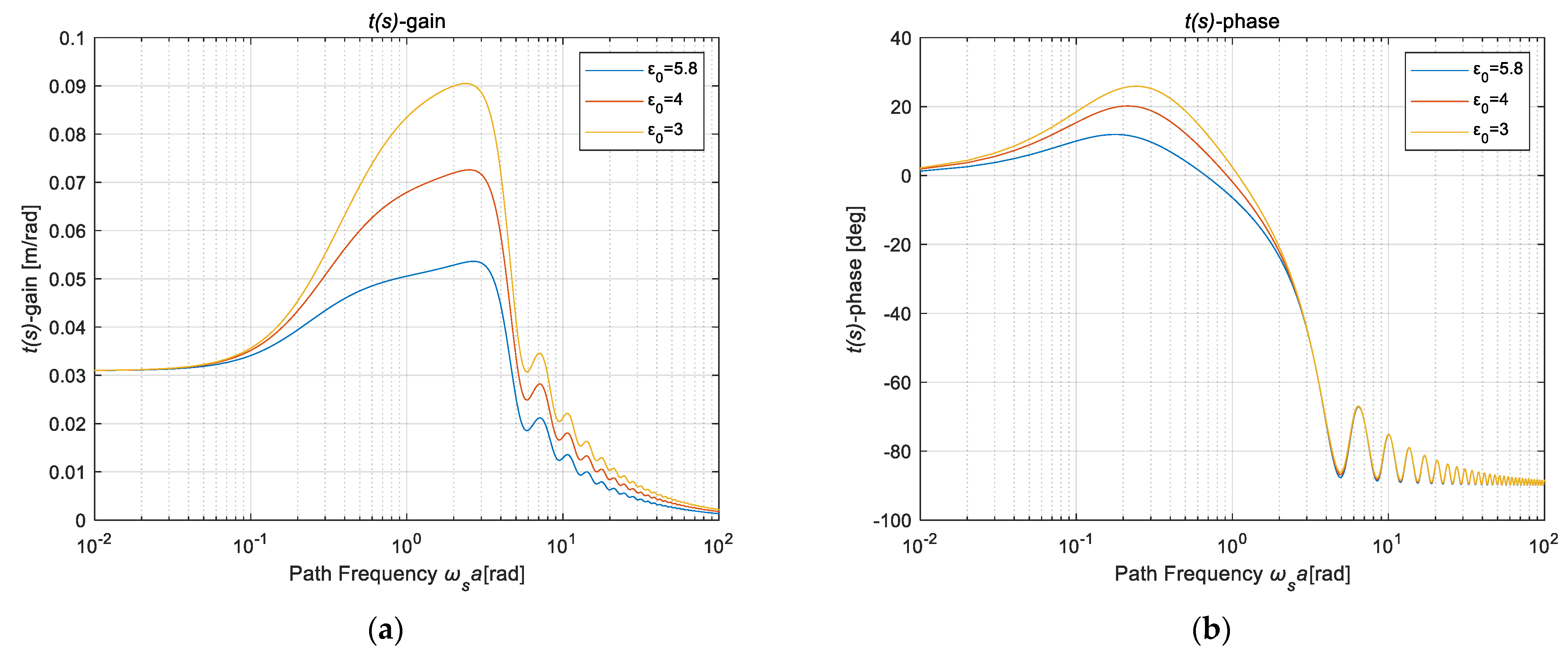
Bringing in the transfer function expressions of lateral force and aligning torque, respectively, the frequency response of the nonlinear pneumatic trail can be obtained. The amplitude–frequency and phase–frequency characteristics are as in the following figure (Figure 9):
This expression is invalid when the slip angle is zero; the steady-state lateral force is zero, so there will be a discontinuity at zero. Stationary gain is now equal to the local derivative of the stationary trajectory with the slip characteristic, which has a discontinuity at zero slip. In Figure 10, the amplitude response exhibits an “overshoot” and two distinct cutoff frequencies at smaller average slip levels. As the slip level increases, the overshoot decreases, while only one cutoff frequency remains. In this case, the response function behaves as a first-order system over the entire frequency range.
After considering the complex deformation of the carcass, the transient response of the pneumatic trail still retains its basic characteristics. Because the elasticity of the carcass affects the cut-off frequency of the original first-order relaxation, the pneumatic trail is further back, and it has a certain inhibitory effect on overshoot. However, at the same time, due to the influence of the torsion and bending deformation of the carcass, the response of the pneumatic trail after considering the deformation of the carcass becomes extremely complicated, and further analysis is required in the subsequent semi-empirical model development process.
3. Nonlinear Unsteady Dynamic Load Sideslip Semi-Physical Model
The theoretical tire model has many assumptions, and its computational efficiency is low due to the complexity of the model. Therefore, considering the current usage scenario, developing a tire semi-physical model has wider practical value, and the semi-physical model usually has high computational efficiency, which is especially suitable for vehicle electronic control system development and performance simulation analysis.
3.1. Nonlinear Unsteady Semi-Physical Model of Tire Lateral Force
According to the unsteady sideslip theoretical model developed above, the frequency response functions of the lateral force and the aligning torque can be obtained. However, because the functions are too complex, further simplification is required to obtain a practical semi-physical model framework. The simplification process mainly includes two aspects; one is only considering the translation deformation of the carcass, and the other is the first-order Taylor expansion of the characteristic function.
Herein:
Therefore, the first-order Taylor expansion of can be obtained:
When s tends to zero, is the local reciprocal of the steady-state lateral force to the slip angle near the position of the effective slip angle , which is defined as the effective cornering stiffness:
Through the previous theoretical analysis, the lateral force shows good first-order behavior at different slip angle levels, so the relaxation length parameter is defined to express the unsteady-state relaxation properties. Among them, is mainly affected by the load and the slip angle levels, and it expresses the effective stiffness of the actual working position, so it is necessary to further introduce the concept of effective sideslip angle .
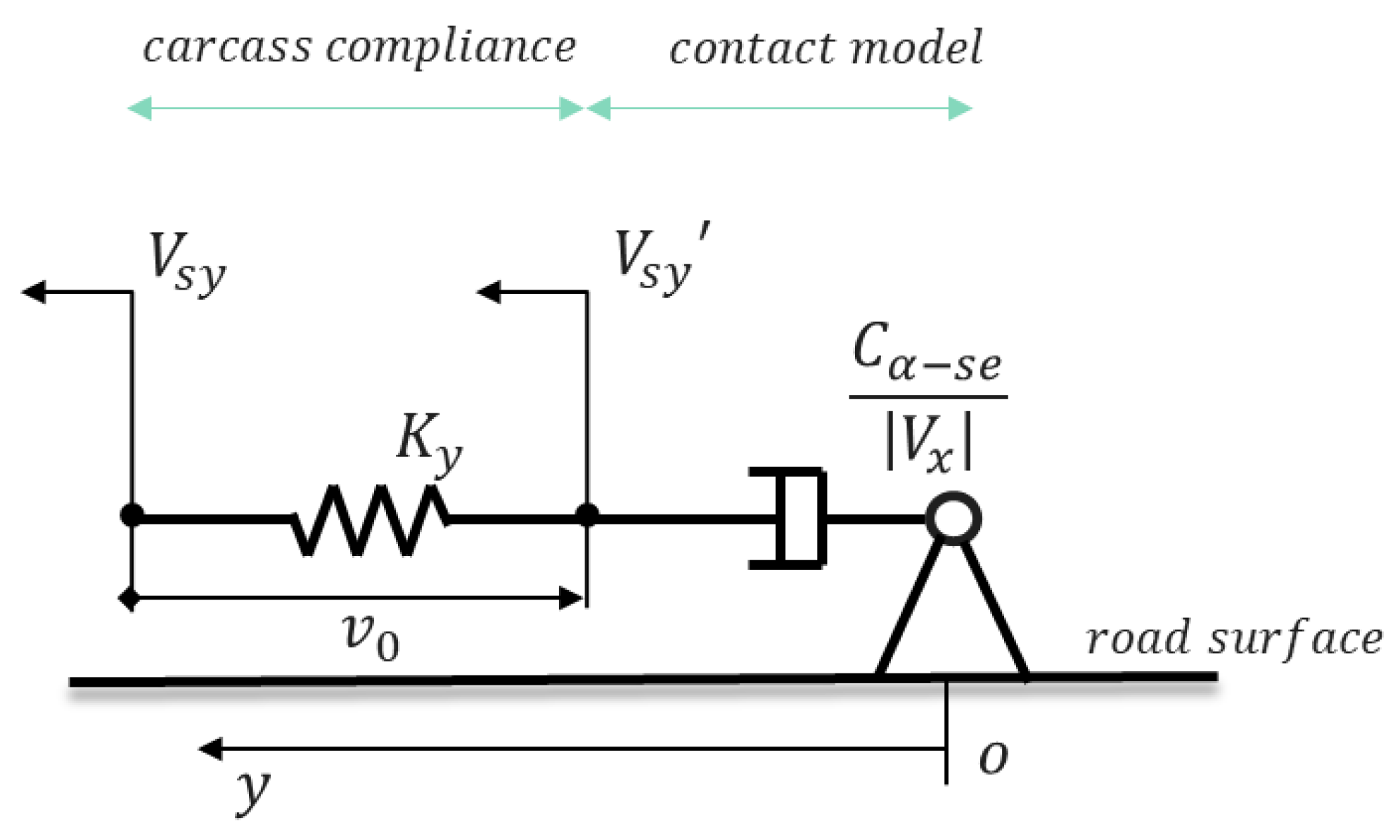
The unsteady sideslip and dynamic load input are jointly introduced into the simplified single-point model for analysis. The schematic diagram of the model is shown below (Figure 11). Note that the analysis of the single-point model is based on the geodetic coordinate system, so the lateral movement speeds of both ends of the carcass are relative to the absolute speed, and the deformation of the carcass is opposite to the sliding direction. Here, the effective lateral slip velocity (the lateral velocity of the lower end of the carcass to the ground) and the transient effective slip angle are introduced:
Define the lateral deformation of the tire carcass, and, according to the node velocity and the carcass deformation, the differential equation of motion is obtained as follows:
Among them, the relationship between the lateral deformation of the carcass and the lateral force is:
In the process of deriving the semi-physical model from the single-point model, two kinds of transient expressions often appear in different papers, and there are often cases of misuse. The key is the application of the two parameters of tire tangential stiffness and secant stiffness , and the two methods are applicable to different working conditions. The following two types of methods will be systematically analyzed.
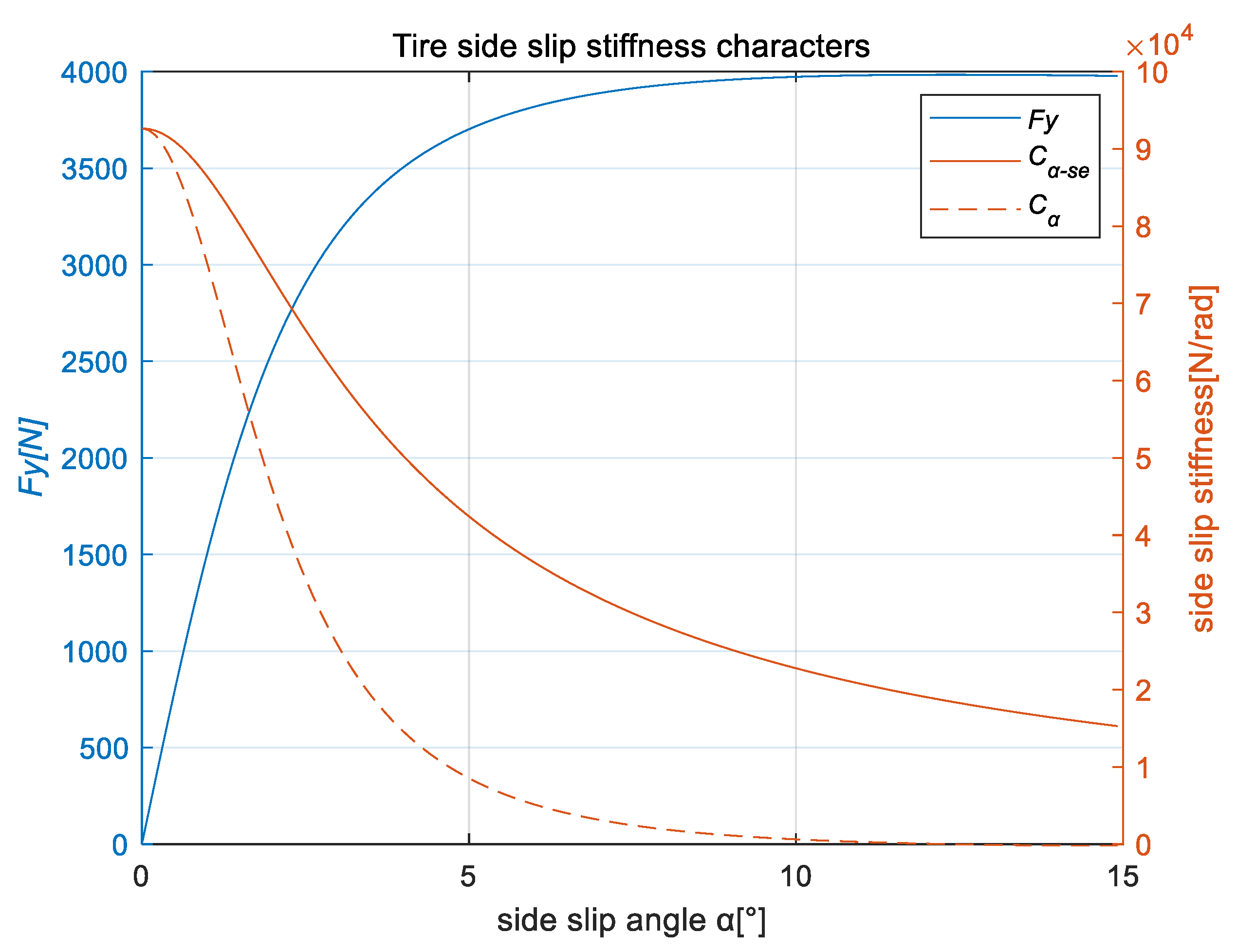
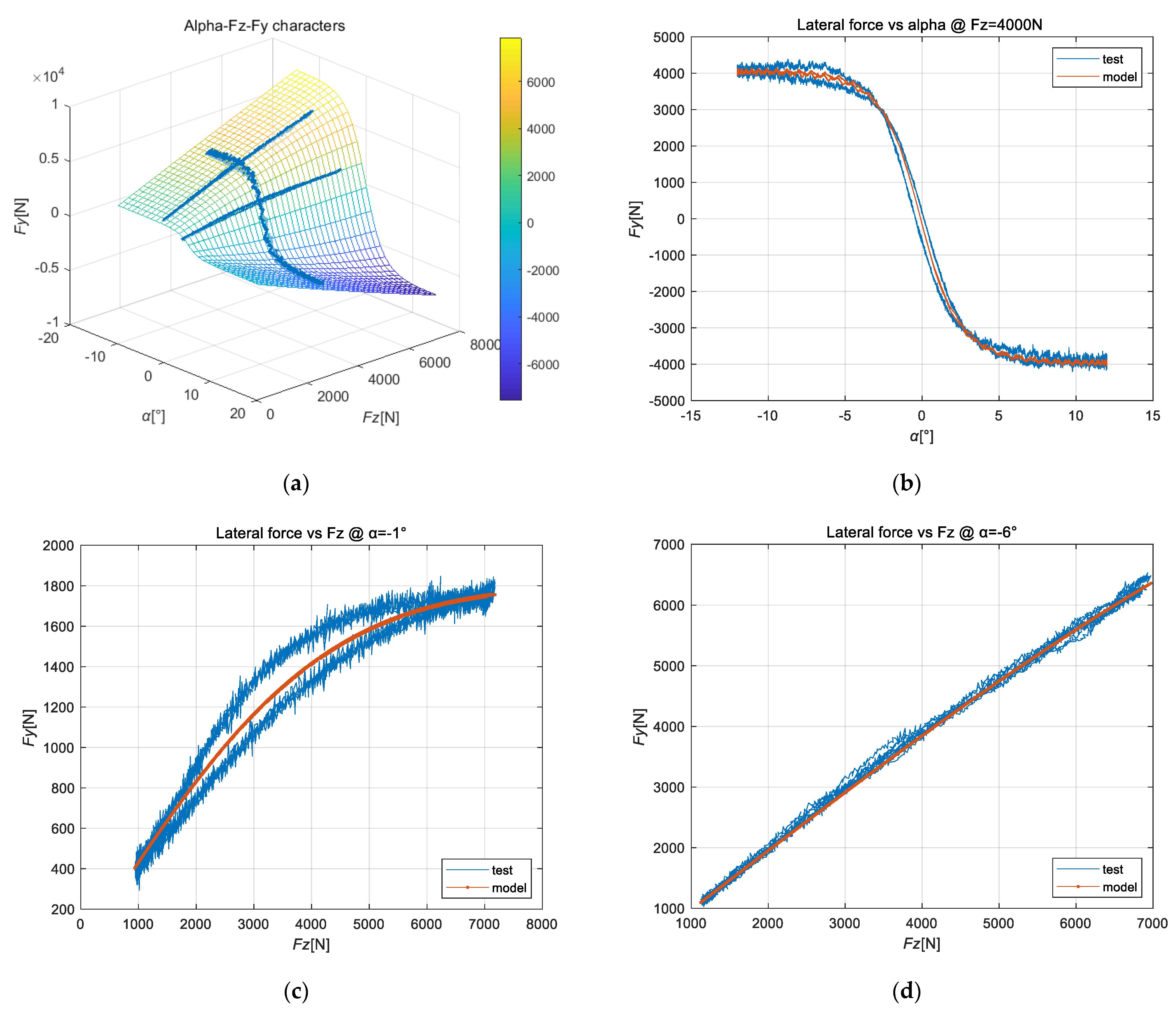
Taking the cornering lateral force characteristics of a 205/55R16 tire as an example (the lateral force is taken as an absolute value for the convenience of observation), it can be seen that the characteristics of the two local cornering stiffness parameters are shown in the figure below (Figure 12). At zero degrees, the secant cornering stiffness and the tangential cornering stiffness tend to be consistent. As the angle increases, the tangential cornering stiffness decreases at a significantly higher rate than the secant stiffness. At the same time, when the lateral force is saturated, the tangent stiffness decreases to almost zero, and the stiffness decreases to negative values when there is a peak in the lateral force:
Method 1.
Considering a constant vertical load, and defining , substituting into the above formula, we have:
Method 2.
Define , substituting into the above formula, we have:
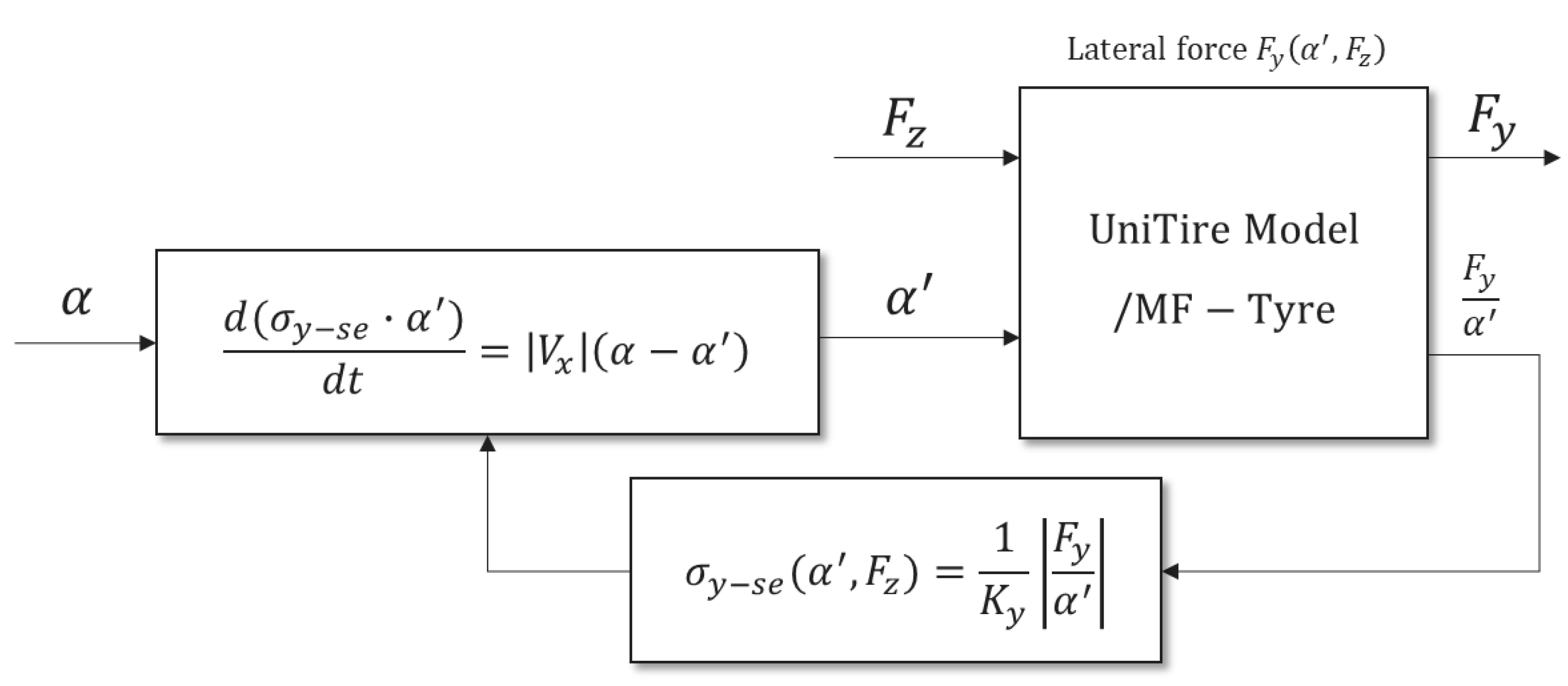
It can be seen from the differential equation that, under the dynamic load condition, the high-frequency fluctuation of the lateral force caused by the load change leads to the deformation speed of the carcass. Therefore, the essence of the dynamic load condition is to show the coupling characteristics of the dynamic load and dynamic sideslip at the same time. Comparing the two methods of expressing the first-order relaxation characteristics, the second method can be relatively simple to be used in the working conditions that take into account both dynamic load and dynamic sideslip. This method is an implicit differential iterative method; its simulation calculation block diagram is as in following figure (Figure 13). The UniTire Model and MF-Tyre are semi-empirical steady-state tire model, which is based on a set of mathematical expressions to represent experimental tire data and have high expression precision.
3.2. Nonlinear Unsteady Semi-Physical Model of Tire Aligning Torque
According to the analysis results of the previous theoretical model, it can be seen that the response is relatively complex (second-order behavior near zero sideslip and gradually becomes first-order behavior after the level of slip angle increases, accompanied by an “overshoot” phenomenon), which is not a simple first-order system and needs to be further decomposed. First, the original steady-state sideslip model system is used to express the aligning torque as the product of the lateral force and the pneumatic trail (negative), so it is necessary to analyze the response of the pneumatic trail. Therefore, the expression of the pneumatic trail is further simplified, and the dimensionless first-order characteristic expression of the lateral force is extracted.
The empirical expression for the response of the pneumatic trail can be defined as a typical second-order system with zeros
Define the system parameter return to pneumatic trail gain as , zero-point parameter , second pole parameter , related to the effective sideslip angle position. Compare the empirical expression with the theoretical model and analyze the functional expression of each empirical parameter (introduce the parameter to be identified):
According to the above formula, its system gain is the local partial derivative of the sideslip angle of the pneumatic trail, so it can be considered as a standard second-order system with zero-point input to the opposite sideslip angle. At the same time, its system gain is the local partial derivative of the pneumatic trail of the steady-state model. Therefore, when developing a semi-physical model, analogous to the modeling process of the lateral force, the response of the pneumatic trail can be inversely transformed into a standard differential equation, and the effective sideslip angle of the pneumatic trail can be expressed by series and coupling superposition and then transmitted to the steady-state model.
In the semi-physical model, the slip point parameter can be empirically expressed as a function of the peak lateral force at the working state position and the cornering stiffness at zero slip angle .
An empirical relationship is established between the second pole parameter (corresponding to the secant stiffness) and the lateral relaxation length, and the parameter m to be identified is introduced:
According to the frequency response function of the pneumatic trail , it is divided into a series of two first-order systems, and the zero-point and the second pole are decomposed at the same time, and the following two first-order differential equations are obtained after further sorting.
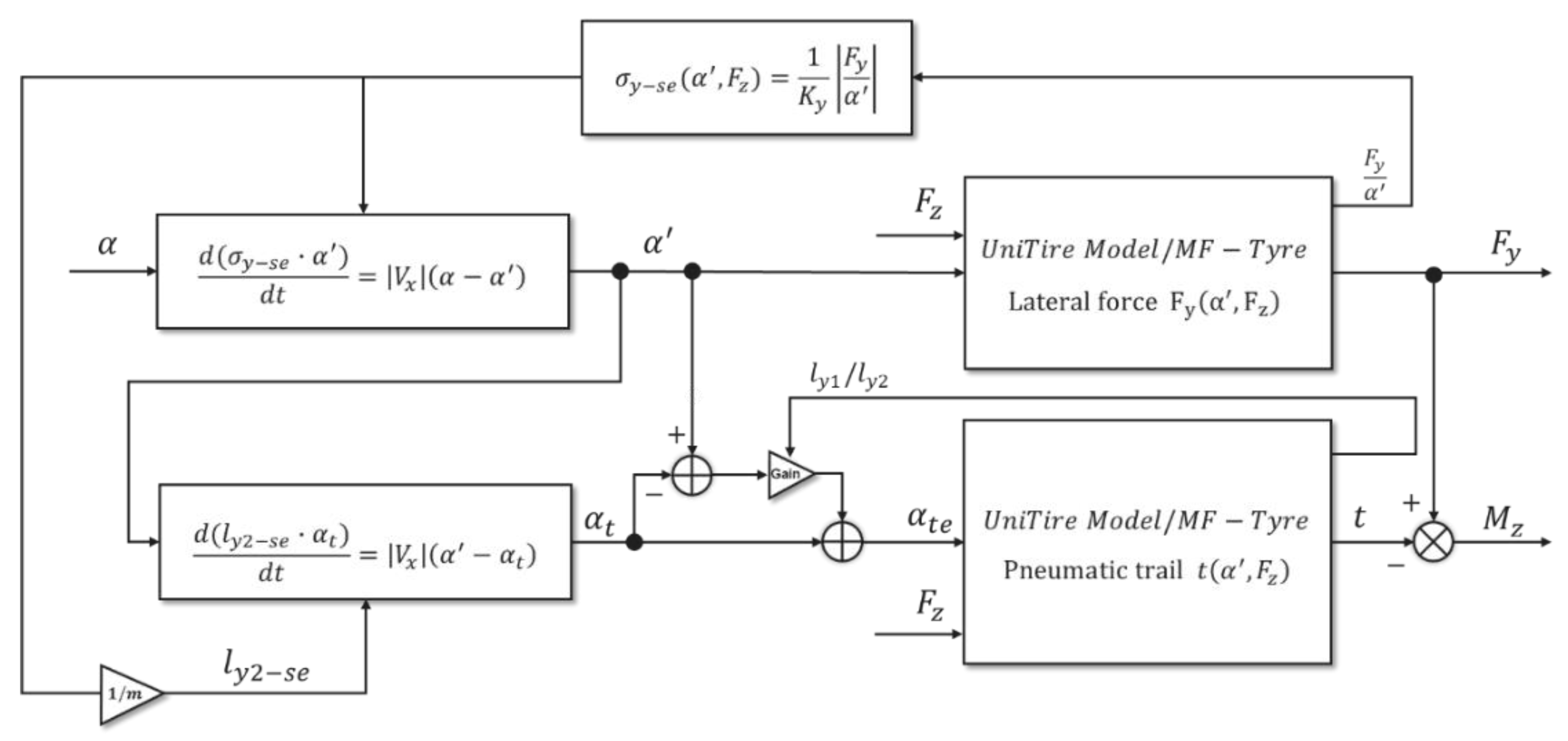
Through the series connection of differential equations, signal feedback, and coupling superposition correction, the effective sideslip angles of the lateral force and the pneumatic trail are obtained, and, based on the steady-state lateral force and aligning torque model, the unsteady lateral force and aligning torque under the input conditions of dynamic load and unsteady sideslip coupling change can be calculated. Its simulation calculation block diagram is shown in the figure (Figure 14).
4. Results and Discussion
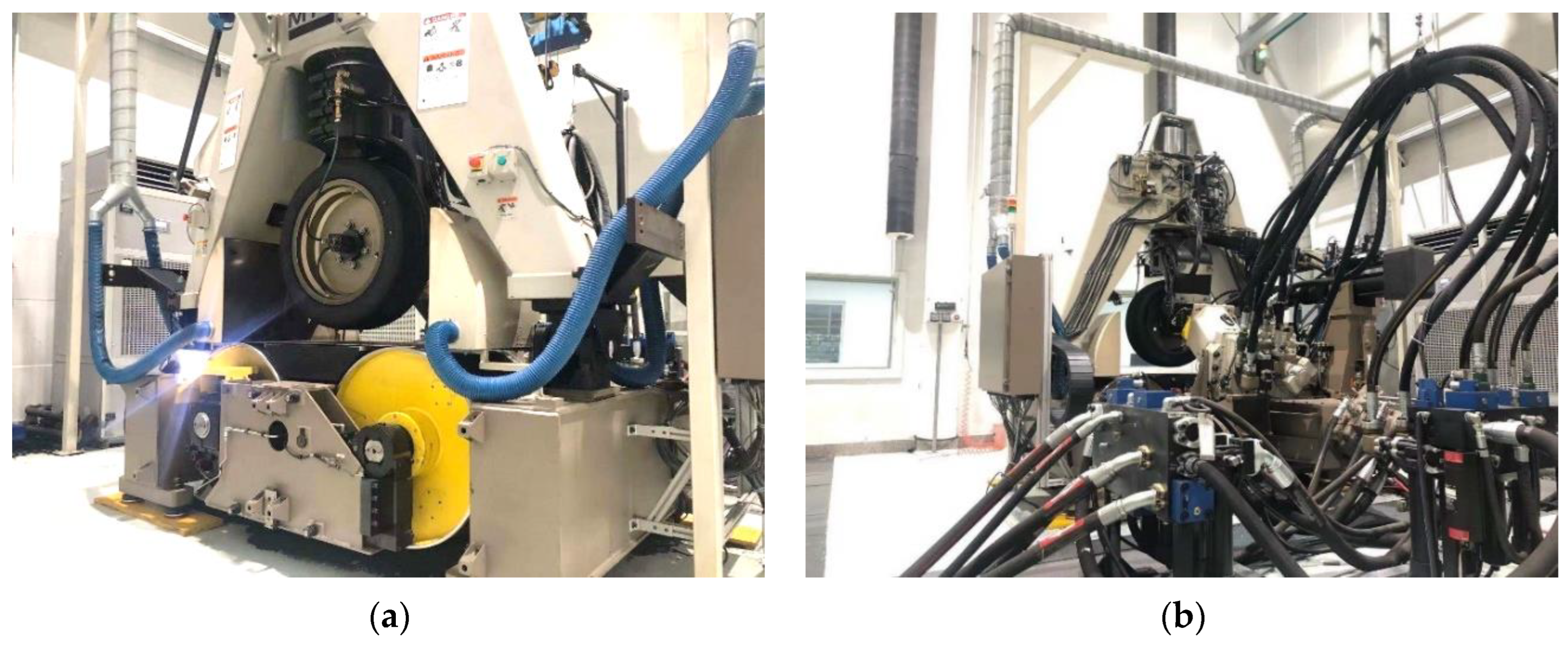
In order to verify the tire model under the condition of unsteady cornering dynamic load input, this section will conduct a large number of unsteady and dynamic cornering mechanical characteristics tests on an indoor tire testing machine. The testing machine used is MTS flat-trac CT III (Figure 15), which can provide high-quality modeling test data for tire models required for high-precision virtual simulation of vehicles. The MTS flat-trac series testing machine is the most advanced and widely used tire six-component force characteristic test system in the world.
This cornering characteristic test mainly includes three categories, quasi-steady cornering characteristic test, slip angle step test, and dynamic load cornering test. There is one item that has a great influence on the expression of transient characteristics: road speed, through the previous theoretical model research, it can be known that the equivalent path frequency is positively correlated with the loading frequency and negatively correlated with the road speed, so reducing the road speed can greatly improve the path frequency input. Therefore, considering the actual control level of the testing machine, the road speed is selected as 5 km/h, which is analogous to 12 times the path frequency under the condition of loading frequency of 60 km/h common vehicle speed at the same time. Refer to the following tables (Table 1, Table 2 and Table 3) for detailed test conditions:
4.1. Characteristic Identification of Tire Steady-State Cornering Lateral Force and Realigning Moment for Dynamic Load Research
In order to verify the response of the model under the unsteady dynamic load cornering condition, the steady-state cornering lateral force and the aligning torque model should be obtained first. Since the expression of the empirical model needs to rely on sufficient experimental data, the quasi-steady-state cornering method (Table 1) can make the model more accurate in the expression of dynamic load conditions.
4.2. Characteristic Identification of Nonlinear Unsteady Sideslip Lateral Force and Aligning Torque
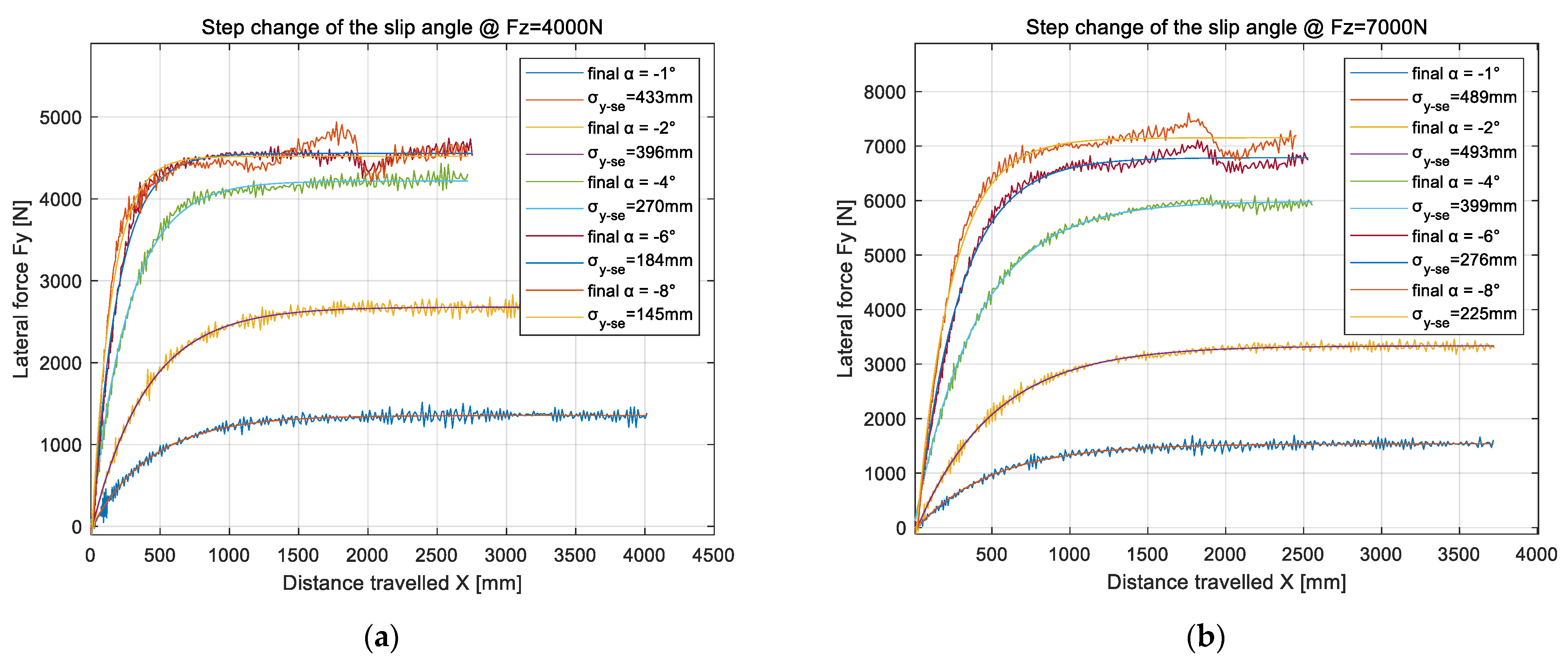
In order to verify the unsteady response of the tire slip angle step in the space domain under different loads and different final slip angles, a combined test of four loads and five final slip angles was carried out. Firstly, the basic identification of the unsteady response characteristics of the lateral force is carried out, considering that the lateral force is a typical approximate first-order response. The state process is faster, so the general solution of the differential equation under the step input condition is still used to identify the relaxation length under each condition, as shown in the following figure (Figure 18) (two loads as an example).
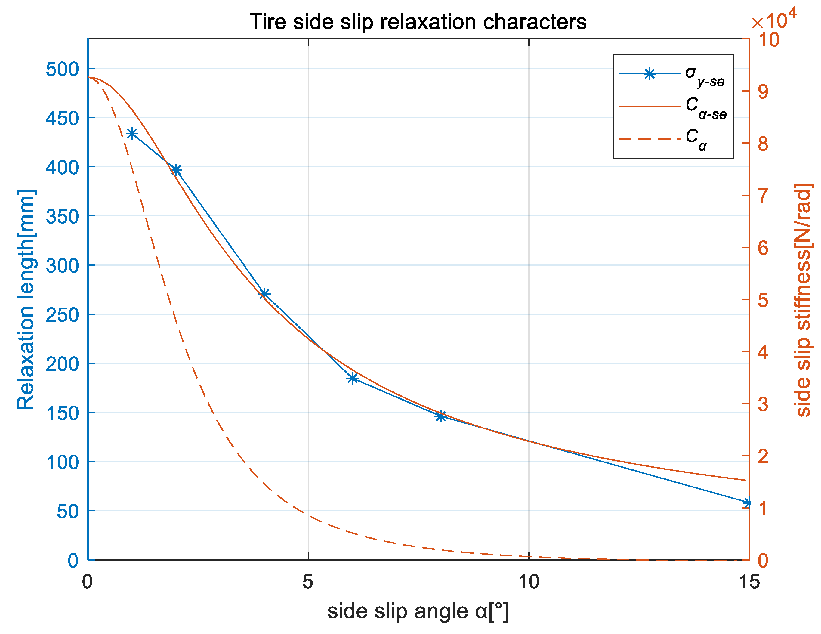
According to the previous theoretical research, the lateral relaxation length obtained by this method is compared with the secant stiffness and the tangent stiffness in a dimensionless manner, as shown in the figure below (Figure 19). By sorting out the identification results of the relaxation length of the slip angle step, the parameter to be identified can be obtained. In the unsteady expression of the lateral force, only this parameter needs to be identified, and practical numerical simulation can be carried out relying on the steady-state model.
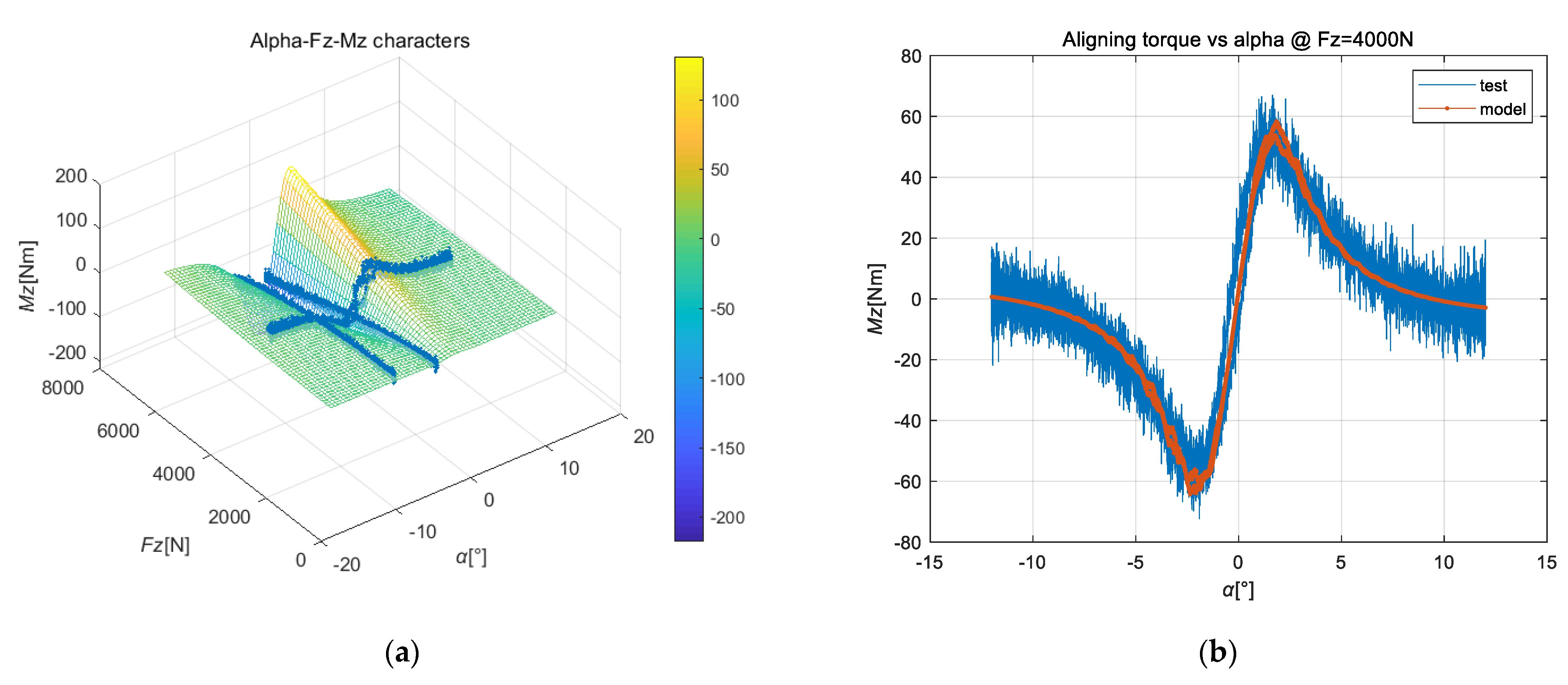
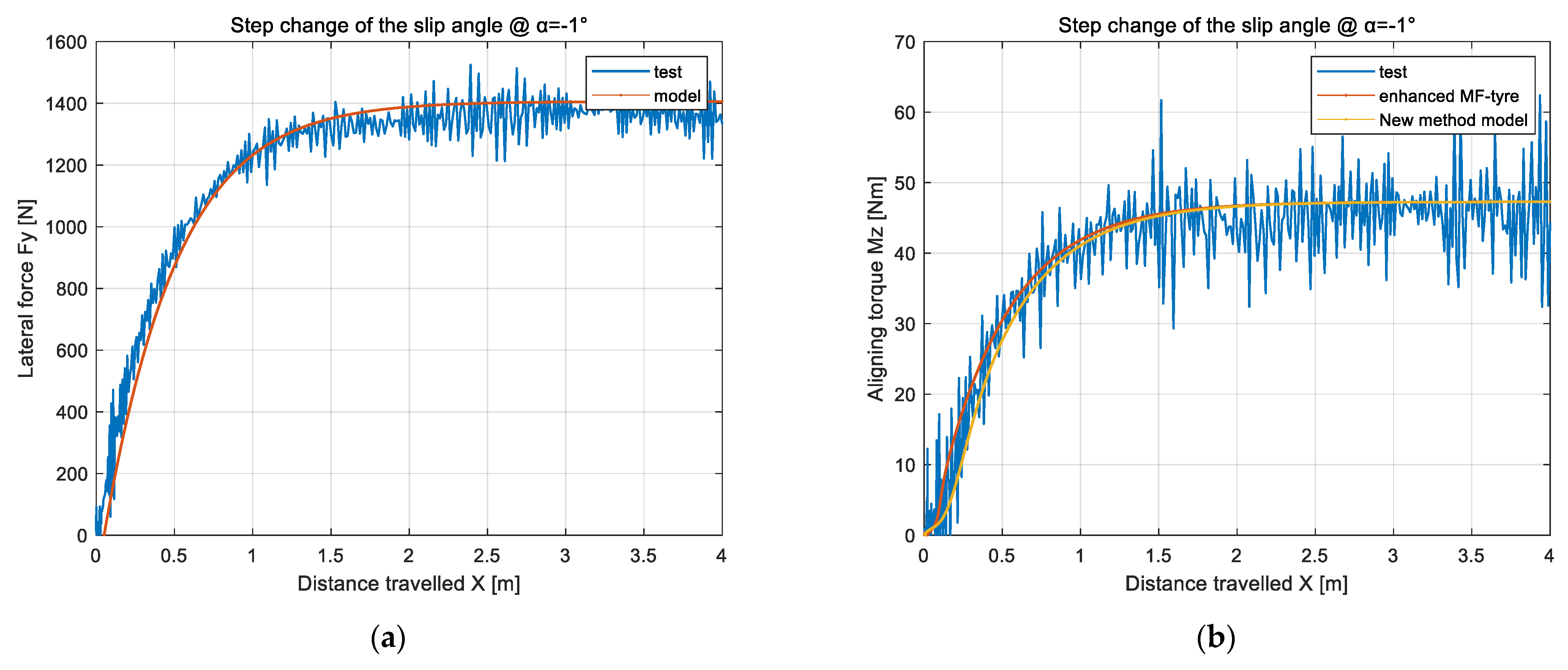
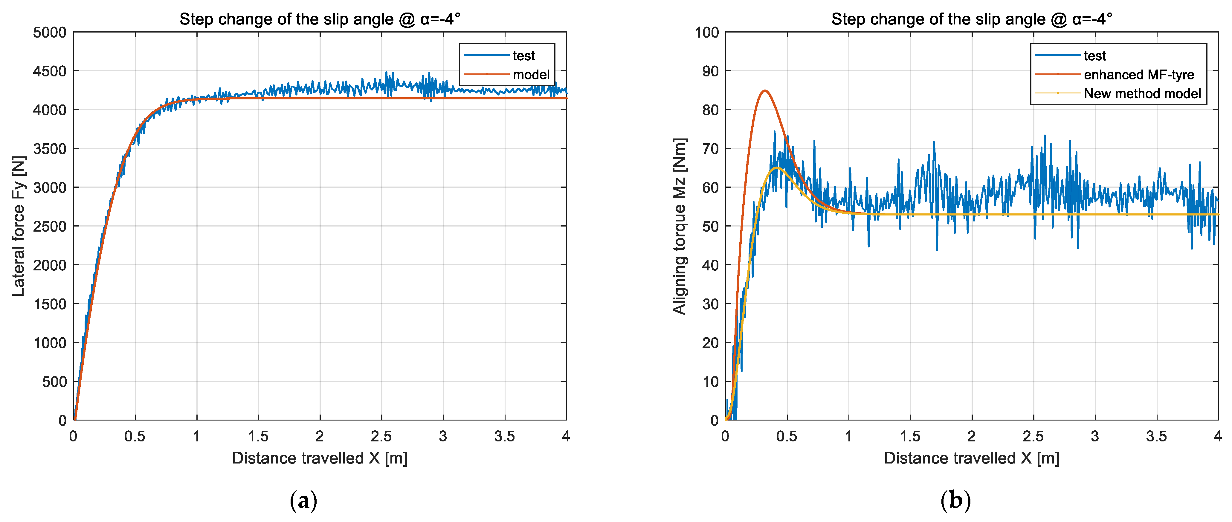
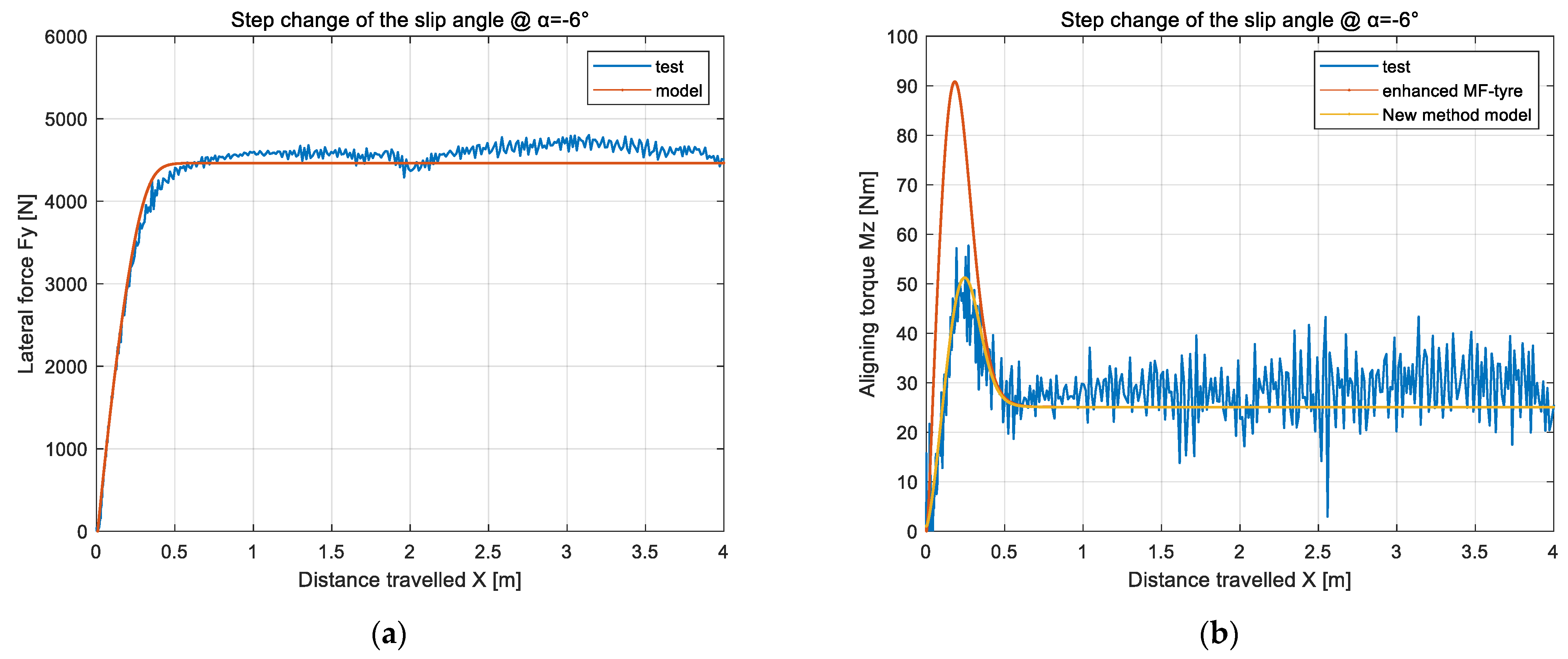
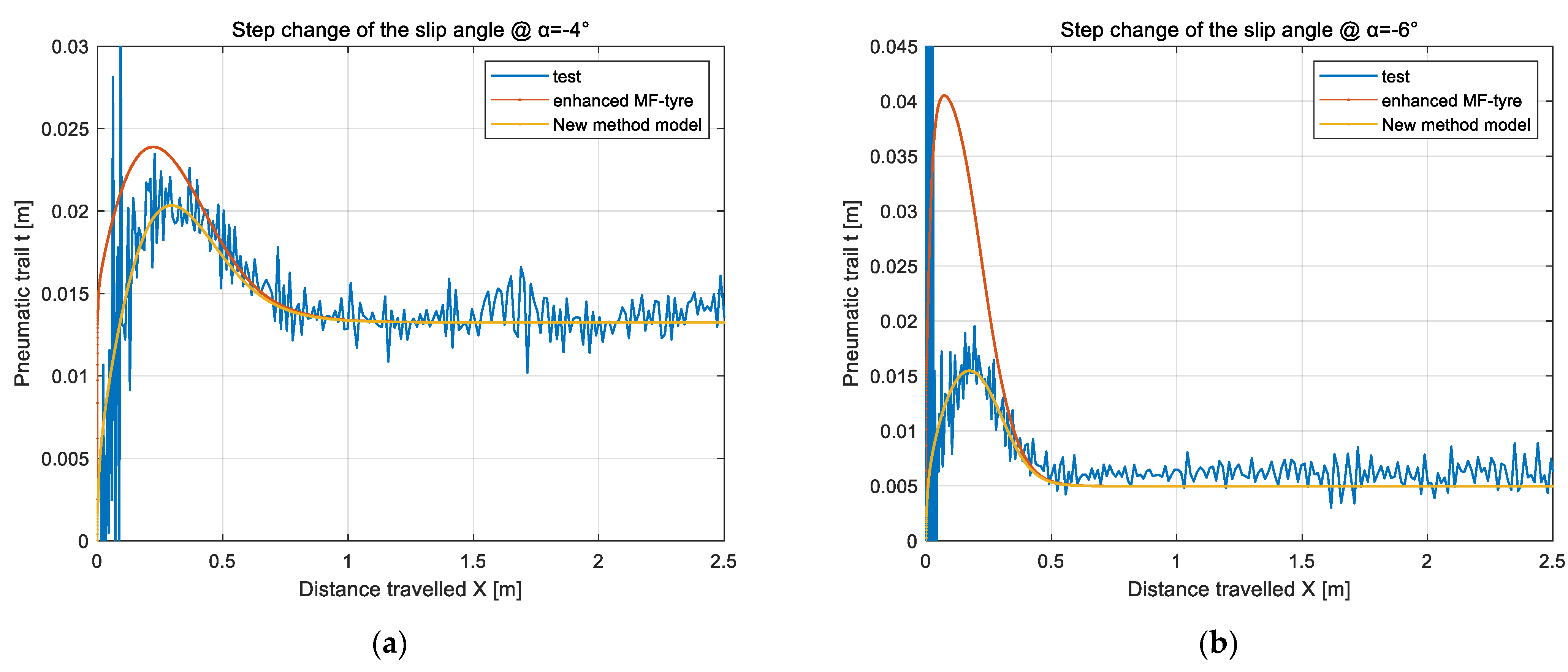
Based on the test data, two key correction parameters, and are identified for the pneumatic trail; it can be seen that the new model has a good improvement in the expression of the aligning torque and can accurately express the changing process of the aligning torque in the space domain from the below figures (Figure 20, Figure 21 and Figure 22).
The key to the improvement in the aligning torque is to have a more accurate expression for the pneumatic trail (Figure 23). When the step lateral force is gradually established, the distribution of the lateral force is gradually transformed from a relatively uniform rectangle to a trapezoid, and it finally reaches a triangle (assuming all the tire treads are attached), so, during this process, the pneumatic trail should gradually increase from zero to the peak. When the slip is considered, since the effective sideslip angle gradually increases to the saturation region, the pneumatic trail will decrease, showing a trend of first increasing and then decreasing. The improved model can accurately express the pneumatic trail transformation.
4.3. Characteristic Identification of Dynamic Load Sideslip Conditions Lateral Force and Aligning Torque (Linear Region and Nonlinear Region)
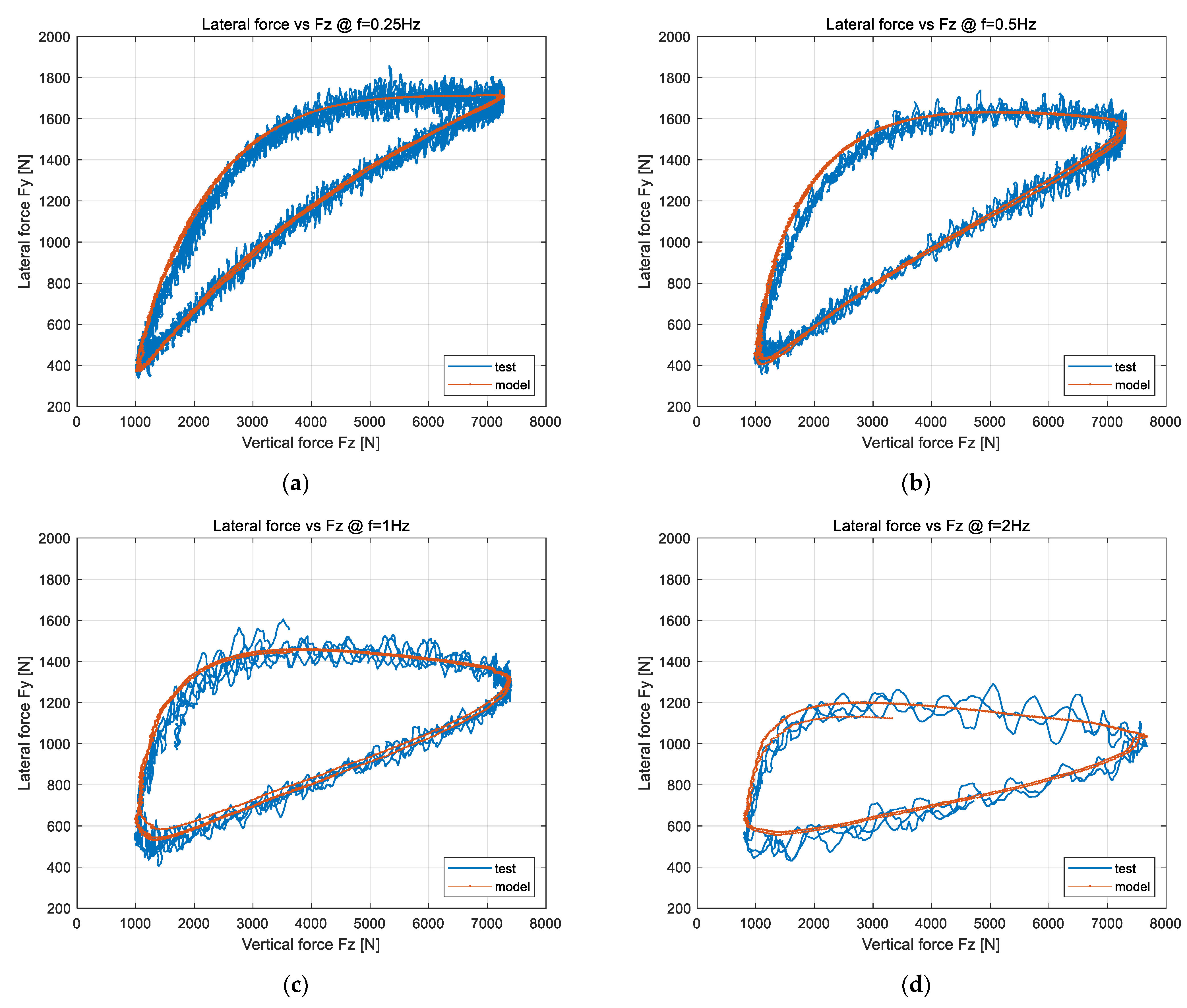
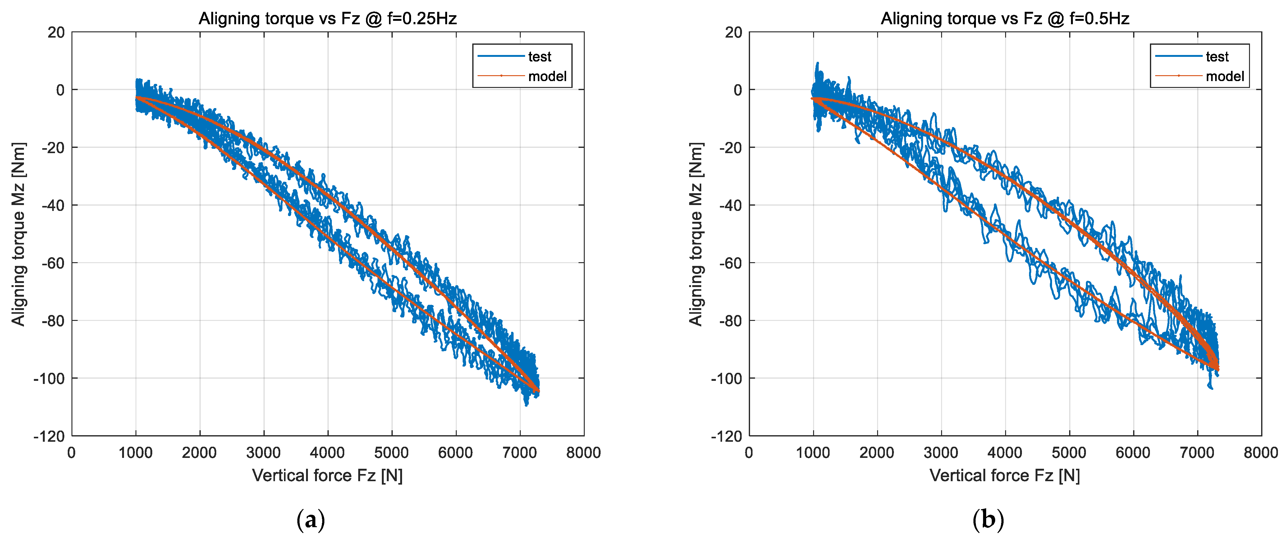
In the vehicle dynamics simulation, the working load of the tire also changes dynamically, and the load has an important influence on the steady and unsteady mechanical properties of the tire. In the process of dynamic loading, its most essential feature is that the change in the load causes a large change in the lateral force, which, in turn, causes a rapid change in the deformation of the carcass, thus making the effective slip angle change drastically. The dynamic load cornering mechanical properties of the linear region and the nonlinear region will be verified in the following.
4.3.1. Verification of Dynamic Load Cornering Lateral Force and Aligning Torque in Linear Region
4.3.2. Verification of Dynamic Load Cornering Lateral Force and Aligning Torque in Nonlinear Region
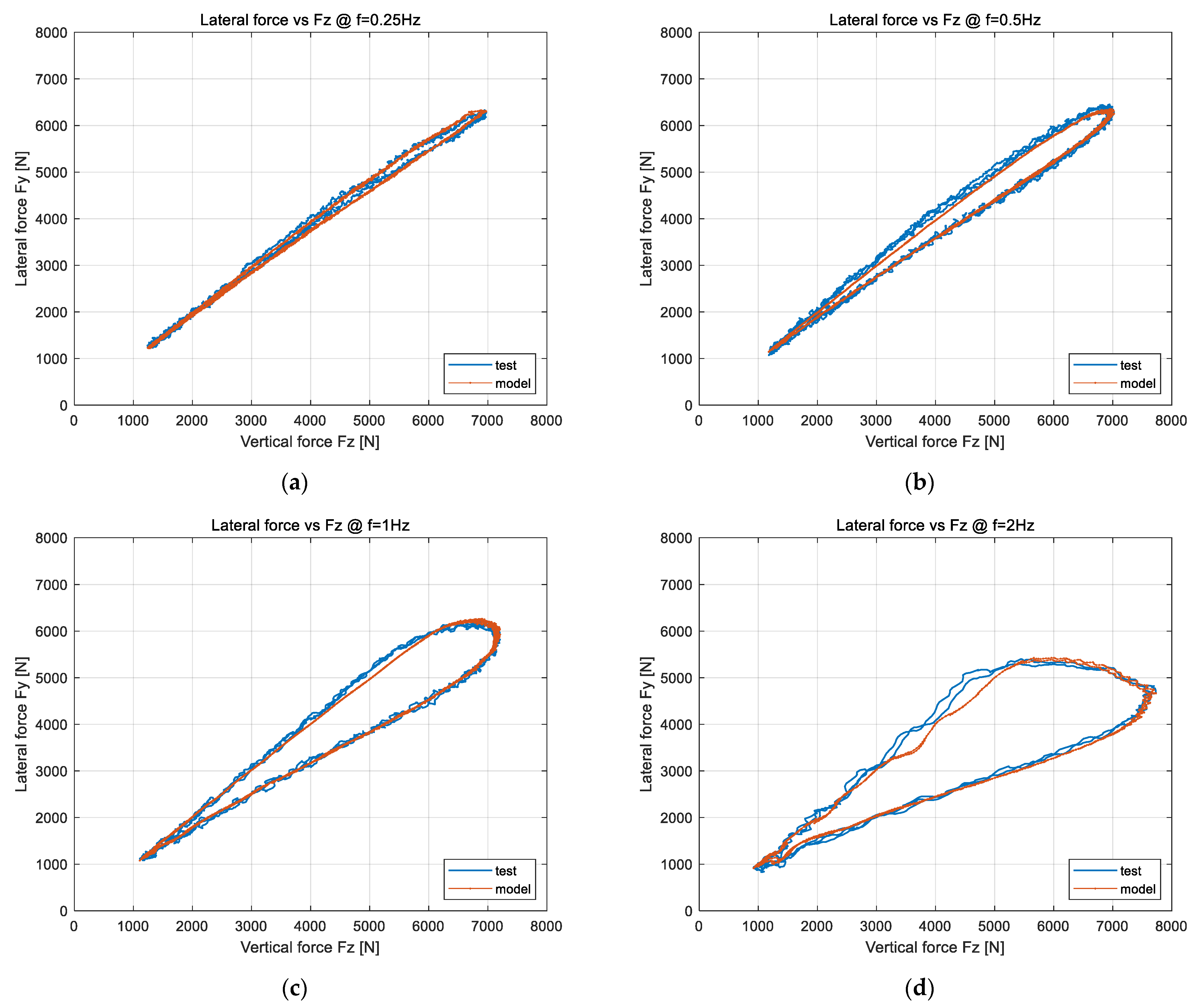
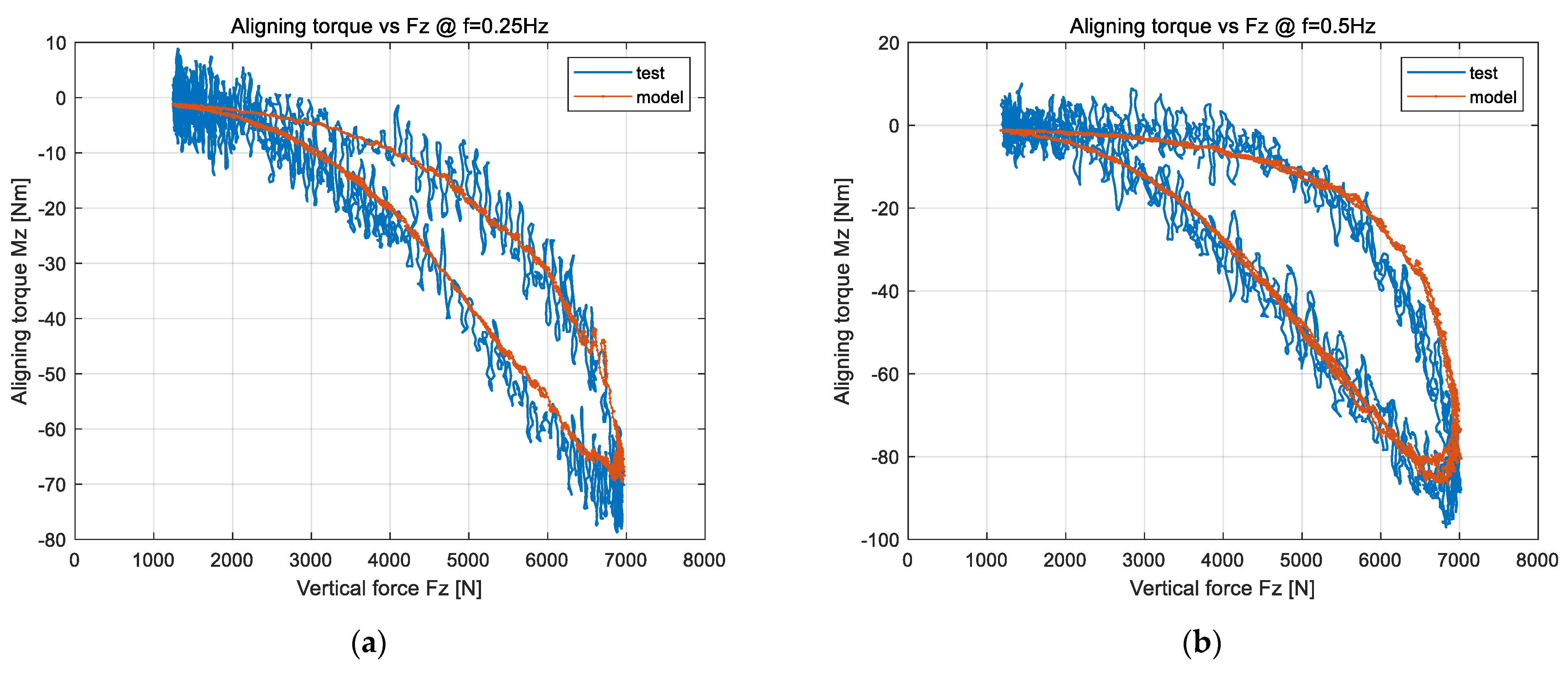
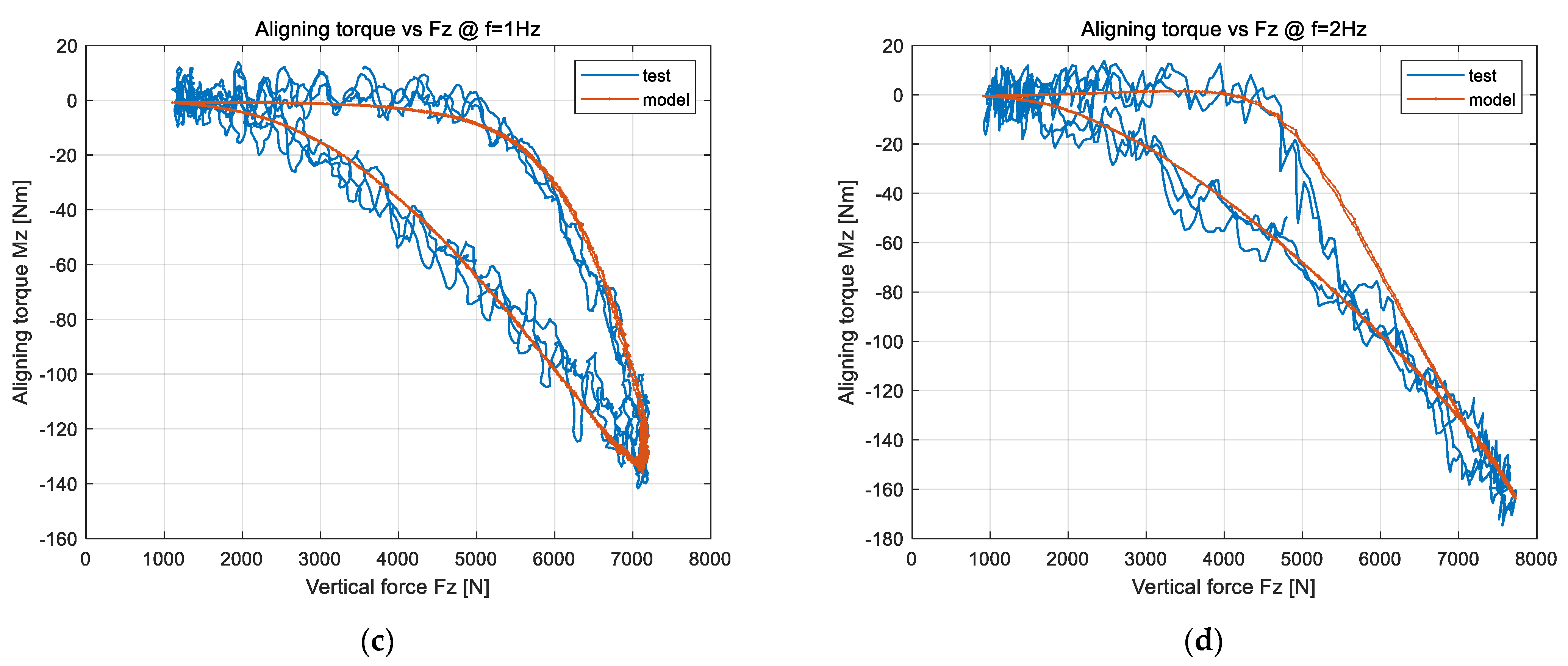
Comparison of unsteady cornering test data and improved semi-physical model simulation results under the condition of constant −6° slip angle and sinusoidal load input occurred (Figure 27, Figure 28 and Figure 29). There are two important differences between the nonlinear region and the linear region. The first is that the operating conditions are generally in a high slip state, so the relaxation length is low and the load and lateral force hysteresis loop is small. The second is that, due to the larger absolute value of the lateral force change, a higher lateral deformation speed of the carcass will be introduced, resulting in a change in the effective slip angle, and the carcass damping effect also needs to be considered at higher frequencies.
It can be seen that lateral force has a very high expression accuracy, and the improved aligning torque model also has a good expression accuracy under the dynamic load input condition. It can be seen that, with the increase in the dynamic load frequency, the aligning torque will increase from −70 Nm~0 to −160 Nm~0, which is mainly due to the effective slip angle change slightly at −6° at low frequency, and it gradually increases to a larger range change so as to greatly increase the pneumatic trail change.
5. Conclusions
This paper systematically analyzed the unsteady tire sideslip characteristics. The paper mainly included three parts. The first part mainly deduced and analyzed the theoretical models of lateral force and aligning torque of tire unsteady characteristics. The second part developed a practical semi-physical tire model. The third part carried out the tire steady and unsteady cornering test and then use the new method model to carry out parameter identification and accuracy verification.
The first part focused on the theoretical analysis of the unsteady mechanical properties of the tire. The theoretical model was extended from the original linear region to the nonlinear region, and the influence of the complex deformation of the carcass was considered. The frequency response function at different sideslip angle levels and its amplitude–frequency and phase–frequency characteristics were analyzed. On this basis, the frequency response of the pneumatic trail was further analyzed and its amplitude–frequency and phase–frequency characteristics were obtained, which provides a reliable theoretical basis for the second part of the unsteady semi-physical model.
The second part first analyzed the nonlinear unsteady model of the lateral force, systematically expounded the theoretical principles and application differences of the two methods (tangential stiffness and secant stiffness), and a unified method was finally determined for the lateral force simulation of dynamic load and sideslip angle. Then, the development of the unsteady semi-physical model of the pneumatic trail was focused on. By decomposing the analytical expression of the theoretical model and analyzing the boundary characteristics, the unsteady semi-physical model was obtained. As an extension module of the steady-state model, the non-steady-state module can be applied to various typical steady-state tire models (UniTire, MF-Tyre, etc.).
In the third part, experiments were carried out to verify the steady-state and unsteady dynamic load characteristics of the sideslip conditions. Then, the key parameters of lateral force (carcass stiffness) and the key parameters (, ) of the pneumatic trail were obtained based on the identification of the step change in the slip angle. The comparison of the experimental data proves that the new method semi-physical model demonstrates great improvement in the expression of the space domain response of the pneumatic trail and the aligning torque. Finally, experiments and simulations were carried out to verify the dynamic load input conditions of different frequencies. Through comparative analysis, the new model can accurately simulate the nonlinear non-steady dynamic load cornering lateral force and aligning torque characteristics of the tire.
In the future, the mechanical characteristics of the combined slip unsteady model will be studied and verified by tests, and a comprehensive tire unsteady dynamic model will be established, which can be fully applied to the simulation of a chassis control system and performance simulation of handling stability and braking, etc.
Author Contributions
Conceptualization, D.L.; methodology, Y.M.; software, H.Y.; validation, Y.M., H.Y. and M.L.; formal analysis, Y.M.; investigation, Y.M.; resources, L.L.; data curation, W.W.; writing—original draft preparation, Y.M.; writing—review and editing, Y.M.; visualization, Y.M.; supervision, D.L.; project administration, D.L.; All authors have read and agreed to the published version of the manuscript.
Funding
This research received no external funding.
Institutional Review Board Statement
Not applicable.
Informed Consent Statement
Not applicable.
Data Availability Statement
Not applicable.
Conflicts of Interest
The authors declare no conflict of interest.
Abbreviations
| Symbol | Description |
| lateral coordinate position of the lower end point of the tread | |
| lateral coordinate position of the lower end point of the carcass | |
| tire lateral force | |
| tire aligning torque | |
| pneumatic trail, time | |
| half contact length | |
| tread element lateral stiffness per unit of length | |
| lateral translational deformation of the carcass | |
| lateral bending deformation of the carcass | |
| lateral torsional deformation of the carcass | |
| lateral translational stiffness of the carcass | |
| lateral bending stiffness of the carcass | |
| lateral torsional stiffness of the carcass | |
| translation deformation feature ratio | |
| bending deformation feature ratio | |
| torsional deformation feature ratio | |
| tire carcass lateral deformation | |
| lateral slip velocity | |
| longitudinal velocity | |
| rolling velocity | |
| sideslip angle | |
| lateral slip velocity on the ground | |
| accumulated time of tread unit movement within contact | |
| longitudinal coordinate of transition from adhesion to sliding | |
| where adhesion occurs | |
| tire parameter of the brush model | |
| path frequency | |
| adhesion parameter | |
| lateral relaxation length | |
| varying part (very small) of sideslip angle | |
| transient tire slip angle | |
| cornering stiffness (tangent) | |
| cornering stiffness (secant) | |
| lateral relaxation length (secant) | |
| pneumatic trail distance constant 1 | |
| pneumatic trail distance constant 2 | |
| pneumatic trail distance constant 2 (secant) | |
| pneumatic trail transient parameter n | |
| pneumatic trail transient parameter m |
References
- Arslan, M.S.; Sever, M. Vehicle stability enhancement and rollover prevention by a nonlinear predictive control method. Trans. Inst. Meas. Control 2019, 41, 2135–2149. [Google Scholar] [CrossRef]
- Van Zanten, A.; Erhardt, R.; Lutz, A. Measurement and Simulation of Transient in Longitudinal and Lateral Tire Forces; SAE Technical Paper 900210; SAE International: Warrendale, PA, USA, 1990; pp. 300–318. [Google Scholar]
- Van Zanten, A.; Erhardt, R.; Landesfeind, K.; Pfaff, G. VDC Systems Development and Perspective. SAE Trans. 1998, 107, 424–444. [Google Scholar]
- Van Zanten, A. Evolution of electronic control systems for improving the vehicle dynamic behavior. In Proceedings of the 6th International Symposium on Advanced Vehicle Control, Hiroshima, Japan, 9–12 September 2002. [Google Scholar]
- Madhusudhanan, A.K.; Corno, M.; Holweg, E. Vehicle yaw rate control using tyre force measurements. In Proceedings of the 2015 European Control Conference (ECC), Linz, Austria, 15–17 July 2015. [Google Scholar]
- Corno, M.; Gerard, M.; Verhaegen, M.; Holweg, E. Hybrid ABS control using force measurement. IEEE Trans. Control Syst. Technol. 2011, 20, 1223–1235. [Google Scholar] [CrossRef]
- Madhusudhanan, A.K.; Corno, M.; Holweg, E. Lateral vehicle dynamics control based on tyre utilization coefficients and tyre force measurements. In Proceedings of the 52nd IEEE Conference on Decision and Control, Florence, Italy, 10–13 December 2013. [Google Scholar]
- Schieschke, R. The importance of tire dynamics in vehicle simulation. In Proceedings of the Tire Society. 9th Annual Meeting and Conference on Tire Science and Technology, Akron, OH, USA, 20–21 March 1990. [Google Scholar]
- Schieschke, R.; Hiemenz, R. The relevance of tire dynamics in vehicle simulation. In Proceedings of the XXIII FISITA Congress, Torino, Italy, 7–11 May 1990. [Google Scholar]
- Luty, W. Simulation research of the tire Basic Relaxation Model in conditions of the wheel cornering angle oscillations. In Proceedings of the IOP Conference Series: Materials Science and Engineering, Bangalore, India, 14–16 July 2016. [Google Scholar]
- Luty, W. Influence of the tire relaxation on the simulation results of the vehicle lateral dynamics in aspect of the vehicle driving safety. J. KONES 2015, 22, 185–192. [Google Scholar] [CrossRef]
- Lozia, Z. Is the representation of transient states of tyres a matter of practical importance in the simulations of vehicle motion? Arch. Automot. Eng.—Arch. Motoryz. 2017, 77, 63–84. [Google Scholar]
- Segel, L. Force and moment response of pneumatic tires to lateral motion inputs. J. Manuf. Sci. Eng. 1966, 88, 37–44. [Google Scholar] [CrossRef]
- Pacejka, H.B. Tire and Vehicle Dynamics, 3rd ed.; Elsevier: Oxford, UK, 2012. [Google Scholar]
- Gong, S. Study of In-Plane Dynamics of Tires. Ph.D. Thesis, Delft University of Technology, Delft, The Netherlands, 1993. [Google Scholar]
- Higuchi, A. Transient Response of Tyres at Large Wheel Slip and Camber. Ph.D. Thesis, Delft University of Technology, Delft, The Netherlands, 1997. [Google Scholar]
- Zegelaar, P.W.A. The Dynamic Response of Tyres to Brake Torque Variations and Road Unevennesses. Ph.D. Thesis, Delft University of Technology, Delft, The Netherlands, 1998. [Google Scholar]
- Maurice, J.P. Short Wavelength and Dynamic Tyre Behaviour under Lateral and Combined Slip Conditions. Ph.D. Thesis, Delft University of Technology, Delft, The Netherlands, 2000. [Google Scholar]
- Schmeitz, A.J.C. A Semi-Empirical Three-Dimensional Model of the Pneumatic Tyre Rolling Over Arbitrarily Uneven Road Surfaces. Ph.D. Thesis, Delft University of Technology, Delft, The Netherlands, 2004. [Google Scholar]
- Besselink, I.J.M. Tire characteristics and modeling. In Vehicle Dynamics of Modern Passenger Cars; Lugner, P., Ed.; Springer: Cham, Switzerland, 2019; Volume 582, pp. 47–108. [Google Scholar]
- Guo, K.; Liu, Q. Modelling and simulation of non-steady state cornering properties and identification of structure parameters of tyres. Veh. Syst. Dyn. 1997, 27 (Suppl. 1), 80–93. [Google Scholar] [CrossRef]
- Pandey, A.; Shaju, A. Modelling transient response using PAC 2002-based tyre model. Veh. Syst. Dyn. 2020, 60, 20–46. [Google Scholar]
- Gipser, M. FTire: A physically based application-oriented tyre model for use with detailed MBS and finite-element suspension models. Veh. Syst. Dyn. 2005, 43 (Suppl. 1), 76–91. [Google Scholar] [CrossRef]
- Février, P.; Blanco Hague, O.; Schick, B.; Miquet, C. Advantages of a thermomechanical tire model for vehicle dynamics. ATZ Worldw. 2010, 112, 33–37. [Google Scholar] [CrossRef]
- Farroni, F.; Giordano, D.; Russo, M.; Timpone, F. TRT: Thermo racing tyre a physical model topredict the tyre temperature distribution. Meccanica 2014, 49, 707–723. [Google Scholar] [CrossRef] [Green Version]
- Sorniotti, A. Tire Thermal Model for Enhanced Vehicle Dynamics Simulation; SAE Technical Paper (No. 2009-01-0441); SAE International: Warrendale, PA, USA, 2009. [Google Scholar]
- Farroni, F.; Sakhnevych, A.; Timpone, F. An evolved version of thermo racing tyre for real time applications. In Lecture Notes in Engineering and Computer Science. In Proceedings of the World Congress on Engineering (WCE), London, UK, 15–17 July 2015. [Google Scholar]
- Beregi, S.; Takacs, D.; Gyebroszki, G.; Stepan, G. Theoretical and experimental study on the nonlinear dynamics of wheel-shimmy. Nonlinear Dyn. 2019, 98, 2581–2593. [Google Scholar] [CrossRef] [Green Version]
- Beregi, S.; Takacs, D.; Stepan, G. Bifurcation analysis of wheel shimmy with non-smooth effects and time delay in the tyre–ground contact. Nonlinear Dyn. 2019, 98, 841–858. [Google Scholar] [CrossRef] [Green Version]
- Beregi, S.; Takács, D. Analysis of the tyre–road interaction with a non-smooth delayed contact model. Multibody Syst. Dyn. 2019, 45, 185–201. [Google Scholar] [CrossRef] [Green Version]
- Romano, L. Advanced Brush Tyre Modelling; Springer: Cham, Switzerland, 2022. [Google Scholar]
- Romano, L.; Sakhnevych, A.; Strano, S.; Timpone, F. A novel brush-model with flexible carcass for transient interactions. Meccanica 2019, 54, 1663–1679. [Google Scholar] [CrossRef] [Green Version]
- Romano, L.; Bruzelius, F.; Jacobson, B. Unsteady-state brush theory. Veh. Syst. Dyn. 2021, 59, 1643–1671. [Google Scholar] [CrossRef]
- Canudas-de-Wit, C.; Tsiotras, P.; Velenis, E.; Basset, M.; Gissinger, G. Dynamic friction models for road/tire longitudinal interaction. Veh. Syst. Dyn. 2003, 39, 189–226. [Google Scholar] [CrossRef]
- Tsiotras, P.; Velenis, E.; Sorine, M. A LuGre tire friction model with exact aggregate dynamics. Veh. Syst. Dyn. 2004, 42, 195–210. [Google Scholar] [CrossRef]
- Velenis, E.; Tsiotras, P.; Canudas-De-Wit, C.; Sorine, M. Dynamic tyre friction models for combined longitudinal and lateral vehicle motion. Veh. Syst. Dyn. 2005, 43, 3–29. [Google Scholar] [CrossRef]
Figure 1.
Tire unsteady motion coordinate system and deformation expression considering carcass deformation (nonlinear).
Figure 1.
Tire unsteady motion coordinate system and deformation expression considering carcass deformation (nonlinear).

Figure 2.
Lateral force frequency characteristic curve at different slip angle positions (rigid carcass): (a) amplitude–frequency; (b) phase–frequency.
Figure 2.
Lateral force frequency characteristic curve at different slip angle positions (rigid carcass): (a) amplitude–frequency; (b) phase–frequency.

Figure 3.
Aligning moment frequency characteristic curve at different slip angle positions (rigid carcass): (a) amplitude–frequency; (b) phase–frequency.
Figure 3.
Aligning moment frequency characteristic curve at different slip angle positions (rigid carcass): (a) amplitude–frequency; (b) phase–frequency.

Figure 4.
Amplitude–frequency characteristics of lateral force and aligning torque at different sideslip angle positions (slip angle = 0°): (a) ; (b) .
Figure 4.
Amplitude–frequency characteristics of lateral force and aligning torque at different sideslip angle positions (slip angle = 0°): (a) ; (b) .

Figure 5.
The frequency characteristic curve of the aligning torque at different sideslip angle positions (near the peak value of the aligning torque): (a) amplitude–frequency; (b) phase–frequency.
Figure 5.
The frequency characteristic curve of the aligning torque at different sideslip angle positions (near the peak value of the aligning torque): (a) amplitude–frequency; (b) phase–frequency.

Figure 6.
Lateral force frequency characteristic curve at different slip angle positions (considering the complex deformation of the carcass): (a) amplitude–frequency; (b) phase–frequency.
Figure 6.
Lateral force frequency characteristic curve at different slip angle positions (considering the complex deformation of the carcass): (a) amplitude–frequency; (b) phase–frequency.

Figure 7.
The frequency characteristic curve of the aligning torque at different slip angle positions (considering the complex deformation of the carcass): (a) amplitude–frequency; (b) phase–frequency.
Figure 7.
The frequency characteristic curve of the aligning torque at different slip angle positions (considering the complex deformation of the carcass): (a) amplitude–frequency; (b) phase–frequency.

Figure 8.
The frequency characteristic curve of the aligning torque at different sideslip angle positions (near the peak value of the aligning torque): (a) amplitude–frequency; (b) phase–frequency.
Figure 8.
The frequency characteristic curve of the aligning torque at different sideslip angle positions (near the peak value of the aligning torque): (a) amplitude–frequency; (b) phase–frequency.

Figure 9.
The frequency characteristic curve of the pneumatic trail at different slip angle positions (rigid carcass): (a) amplitude–frequency; (b) phase–frequency.
Figure 9.
The frequency characteristic curve of the pneumatic trail at different slip angle positions (rigid carcass): (a) amplitude–frequency; (b) phase–frequency.

Figure 10.
The frequency characteristic curve of the pneumatic trail at different slip angle positions (complex deformation of the carcass): (a) amplitude–frequency; (b) phase–frequency.
Figure 10.
The frequency characteristic curve of the pneumatic trail at different slip angle positions (complex deformation of the carcass): (a) amplitude–frequency; (b) phase–frequency.

Figure 11.
Schematic diagram of sideslip single-point tire model.

Figure 12.
Characteristics of tire side force, tangent stiffness, and secant stiffness.

Figure 13.
Block diagram of the single-point model to unsteady-state responses of the lateral force.
Figure 13.
Block diagram of the single-point model to unsteady-state responses of the lateral force.

Figure 14.
Block diagram of the unsteady-state tire model responses of the lateral force and aligning torque.
Figure 14.
Block diagram of the unsteady-state tire model responses of the lateral force and aligning torque.

Figure 15.
MTS flat-trac tire force & moment measurement systems: (a) main view; (b) rear view.

Figure 16.
Tire steady-state lateral force identification results: (a) alpha-Fz-Fy characters; (b) alpha-Fy characters; (c) Fz-Fy characters of −1° slip angle; (d) Fz-Fy characters of −6° slip angle.
Figure 16.
Tire steady-state lateral force identification results: (a) alpha-Fz-Fy characters; (b) alpha-Fy characters; (c) Fz-Fy characters of −1° slip angle; (d) Fz-Fy characters of −6° slip angle.

Figure 17.
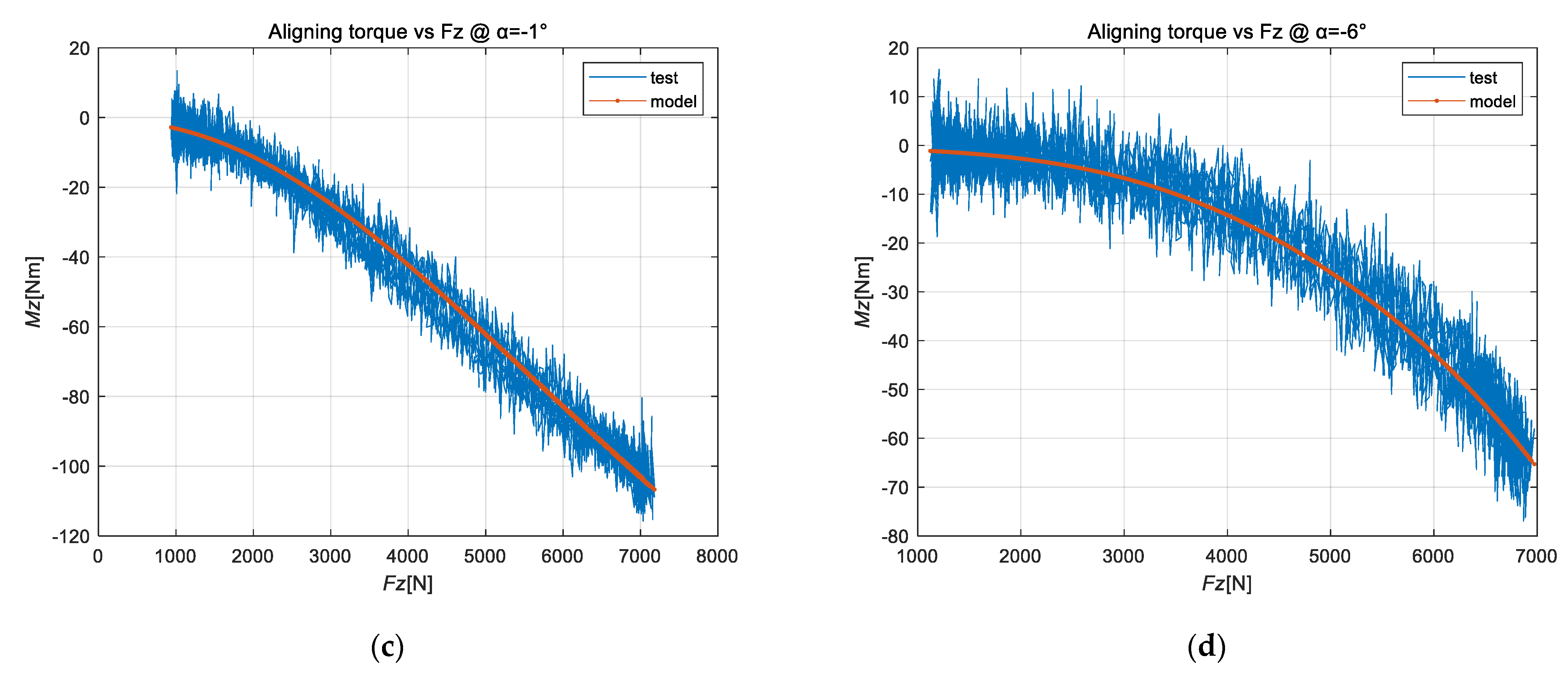
Tire steady-state aligning torque identification results: (a) alpha-Fz-Mz characters; (b) alpha-Mz characters; (c) Fz-Mz characters of −1° slip angle; (d) Fz-Mz characters of −6° slip angle.
Figure 17.
Tire steady-state aligning torque identification results: (a) alpha-Fz-Mz characters; (b) alpha-Mz characters; (c) Fz-Mz characters of −1° slip angle; (d) Fz-Mz characters of −6° slip angle.


Figure 18.
Lateral relaxation length identification results under different final slip angles: (a) slip angle step change @ Fz = 4000 N; (b) slip angle step change @ Fz = 7000 N.
Figure 18.
Lateral relaxation length identification results under different final slip angles: (a) slip angle step change @ Fz = 4000 N; (b) slip angle step change @ Fz = 7000 N.

Figure 19.
Correspondence between simple relaxation length and effective cornering stiffness.

Figure 20.
Identification results of lateral force and aligning torque under the condition of −1° final slip angle (Fz = 4000 N): (a) lateral force; (b) aligning torque.
Figure 20.
Identification results of lateral force and aligning torque under the condition of −1° final slip angle (Fz = 4000 N): (a) lateral force; (b) aligning torque.

Figure 21.
Identification results of lateral force and aligning torque under the condition of −4° final slip angle (Fz = 4000 N): (a) lateral force; (b) aligning torque.
Figure 21.
Identification results of lateral force and aligning torque under the condition of −4° final slip angle (Fz = 4000 N): (a) lateral force; (b) aligning torque.

Figure 22.
Identification results of lateral force and aligning torque under the condition of −6° final slip angle (Fz = 4000 N): (a) lateral force; (b) aligning torque.
Figure 22.
Identification results of lateral force and aligning torque under the condition of −6° final slip angle (Fz = 4000 N): (a) lateral force; (b) aligning torque.

Figure 23.
Identification results of pneumatic trail under the condition of slip angle step change (Fz = 4000 N): (a) −4° final slip angle; (b) −6° final slip angle.
Figure 23.
Identification results of pneumatic trail under the condition of slip angle step change (Fz = 4000 N): (a) −4° final slip angle; (b) −6° final slip angle.

Figure 24.
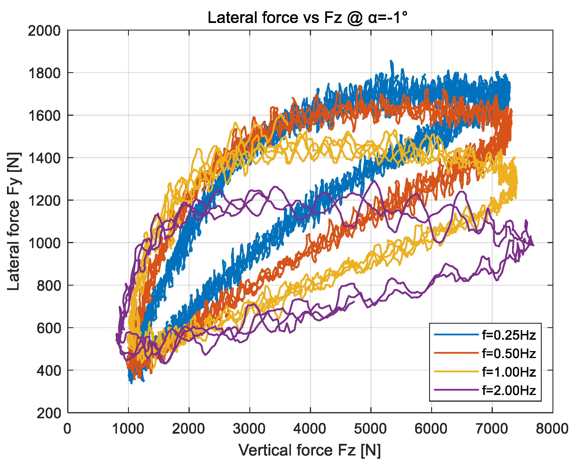
Test results of dynamic load cornering lateral force under the condition of −1° slip angle.
Figure 24.
Test results of dynamic load cornering lateral force under the condition of −1° slip angle.

Figure 25.
Comparison of the relationship between load and lateral force under dynamic load cornering conditions: (a) f = 0.25 Hz; (b) f = 0.50 Hz; (c) f = 1.00 Hz; (d) f = 2.00 Hz.
Figure 25.
Comparison of the relationship between load and lateral force under dynamic load cornering conditions: (a) f = 0.25 Hz; (b) f = 0.50 Hz; (c) f = 1.00 Hz; (d) f = 2.00 Hz.

Figure 26.
Comparison of the relationship between load and aligning torque under dynamic load cornering conditions: (a) f = 0.25 Hz; (b) f = 0.50 Hz; (c) f = 1.00 Hz; (d) f = 2.00 Hz.
Figure 26.
Comparison of the relationship between load and aligning torque under dynamic load cornering conditions: (a) f = 0.25 Hz; (b) f = 0.50 Hz; (c) f = 1.00 Hz; (d) f = 2.00 Hz.


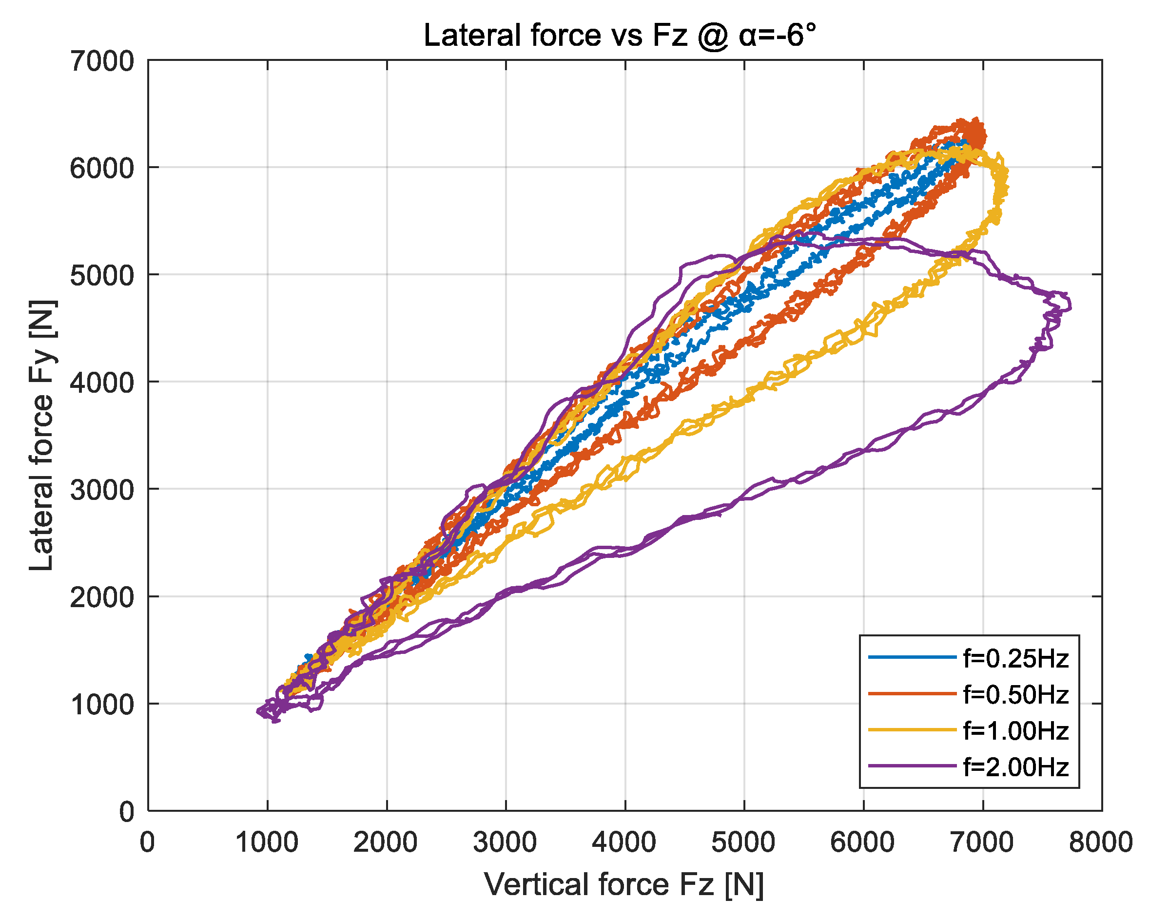
Figure 27.
Test results of dynamic load cornering lateral force under the condition of −6° slip angle.
Figure 27.
Test results of dynamic load cornering lateral force under the condition of −6° slip angle.

Figure 28.
Comparison of the relationship between load and lateral force under dynamic load cornering conditions: (a) f = 0.25 Hz; (b) f = 0.50 Hz; (c) f = 1.00 Hz; (d) f = 2.00 Hz.
Figure 28.
Comparison of the relationship between load and lateral force under dynamic load cornering conditions: (a) f = 0.25 Hz; (b) f = 0.50 Hz; (c) f = 1.00 Hz; (d) f = 2.00 Hz.

Figure 29.
Comparison of the relationship between load and aligning torque under dynamic load cornering conditions: (a) f = 0.25 Hz; (b) f = 0.50 Hz; (c) f = 1.00 Hz; (d) f = 2.00 Hz.
Figure 29.
Comparison of the relationship between load and aligning torque under dynamic load cornering conditions: (a) f = 0.25 Hz; (b) f = 0.50 Hz; (c) f = 1.00 Hz; (d) f = 2.00 Hz.


Table 1.
Quasi-steady-state cornering test condition setting.
| Inflation Pressure | Road Speed | Load Method | Slip Angle | Load Cycle | Vertical Load |
|---|---|---|---|---|---|
| 230 kPa | 5 km/h | Sideslip sweep | −12~12° | 100 s | 4000 N |
| 230 kPa | 5 km/h | Vertical load sweep | −1° | 10 s | 1000~7000 N |
| 230 kPa | 5 km/h | Vertical load sweep | −6° | 10 s | 1000~7000 N |
Table 2.
Nonlinear slip angle step test condition setting.
| Inflation Pressure | Road Speed | Load Method | Slip Angle | Vertical Load |
|---|---|---|---|---|
| 230 kPa | 0→5 km/h | slip angle step | −1° | 3000\4000\5000\7000 N |
| 230 kPa | 0→5 km/h | slip angle step | −2° | 3000\4000\5000\7000 N |
| 230 kPa | 0→5 km/h | slip angle step | −4° | 3000\4000\5000\7000 N |
| 230 kPa | 0→5 km/h | slip angle step | −6° | 3000\4000\5000\7000 N |
| 230 kPa | 0→5 km/h | slip angle step | −8° | 3000\4000\5000\7000 N |
Table 3.
Dynamic load cornering test condition setting.
| Inflation Pressure | Road Speed | Load Method | Slip Angle | Load Frequency | Vertical Load |
|---|---|---|---|---|---|
| 230 kPa | 5 km/h | Vertical load sweep | −1°, −6° | 0.10 Hz | 1000~7000 N |
| 230 kPa | 5 km/h | Vertical load sweep | −1°, −6° | 0.25 Hz | 1000~7000 N |
| 230 kPa | 5 km/h | Vertical load sweep | −1°, −6° | 0.50 Hz | 1000~7000 N |
| 230 kPa | 5 km/h | Vertical load sweep | −1°, −6° | 0.10 Hz | 1000~7000 N |
| 230 kPa | 5 km/h | Vertical load sweep | −1°, −6° | 0.25 Hz | 1000~7000 N |
Publisher’s Note: MDPI stays neutral with regard to jurisdictional claims in published maps and institutional affiliations. |
© 2022 by the authors. Licensee MDPI, Basel, Switzerland. This article is an open access article distributed under the terms and conditions of the Creative Commons Attribution (CC BY) license (https://creativecommons.org/licenses/by/4.0/).
Share and Cite
MDPI and ACS Style
Ma, Y.; Lu, D.; Yin, H.; Li, L.; Lv, M.; Wang, W. The Unsteady-State Response of Tires to Slip Angle and Vertical Load Variations. Machines 2022, 10, 527. https://0-doi-org.brum.beds.ac.uk/10.3390/machines10070527
AMA Style
Ma Y, Lu D, Yin H, Li L, Lv M, Wang W. The Unsteady-State Response of Tires to Slip Angle and Vertical Load Variations. Machines. 2022; 10(7):527. https://0-doi-org.brum.beds.ac.uk/10.3390/machines10070527
Chicago/Turabian StyleMa, Yao, Dang Lu, Hengfeng Yin, Lun Li, Manyi Lv, and Wei Wang. 2022. "The Unsteady-State Response of Tires to Slip Angle and Vertical Load Variations" Machines 10, no. 7: 527. https://0-doi-org.brum.beds.ac.uk/10.3390/machines10070527
Note that from the first issue of 2016, this journal uses article numbers instead of page numbers. See further details here.