
Probabilistic Condition Monitoring of Azimuth Thrusters Based on Acceleration Measurements

 , ,
, ,
Abstract
:1. Introduction
2. Materials and Methods
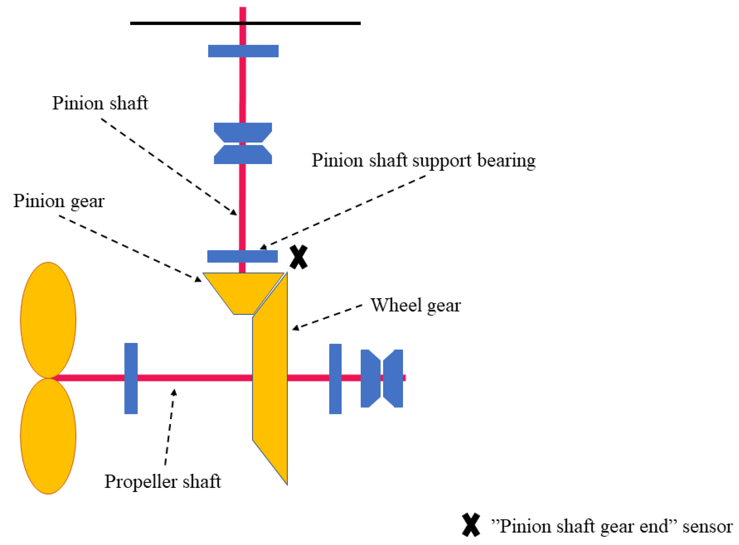
2.1. Azimuth Thruster
2.1.1. Measurements
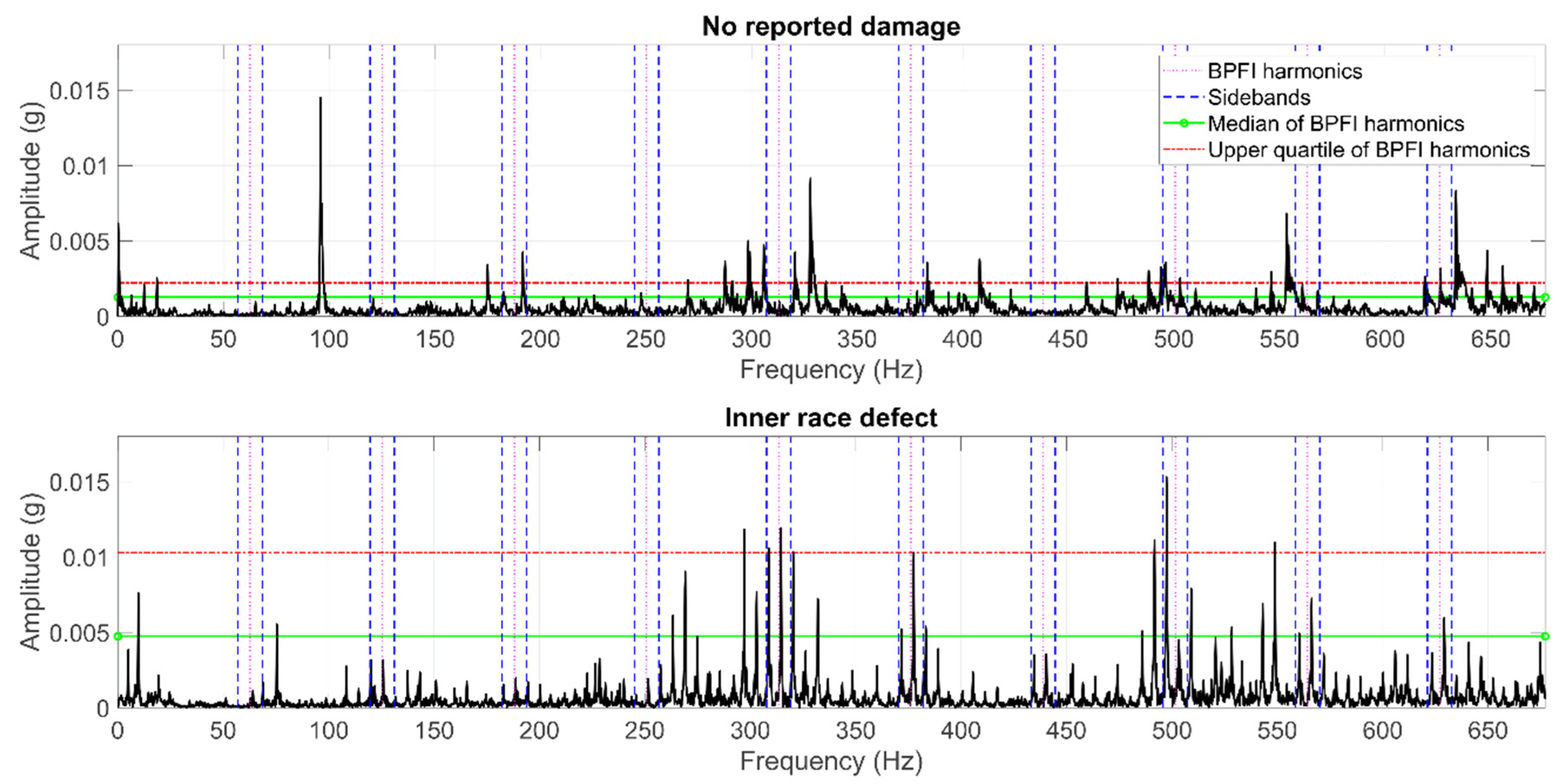
2.1.2. Monitored Components
- Ball Pass Frequency, Inner race (BPFI),
- Ball Pass Frequency, Outer race (BPFO),
- Ball (roller) Spin Frequency (BSF),
- Fundamental Train Frequency–cage speed (FTF), and
- Gear Mesh Frequency (GMF).
2.1.3. Data Selection
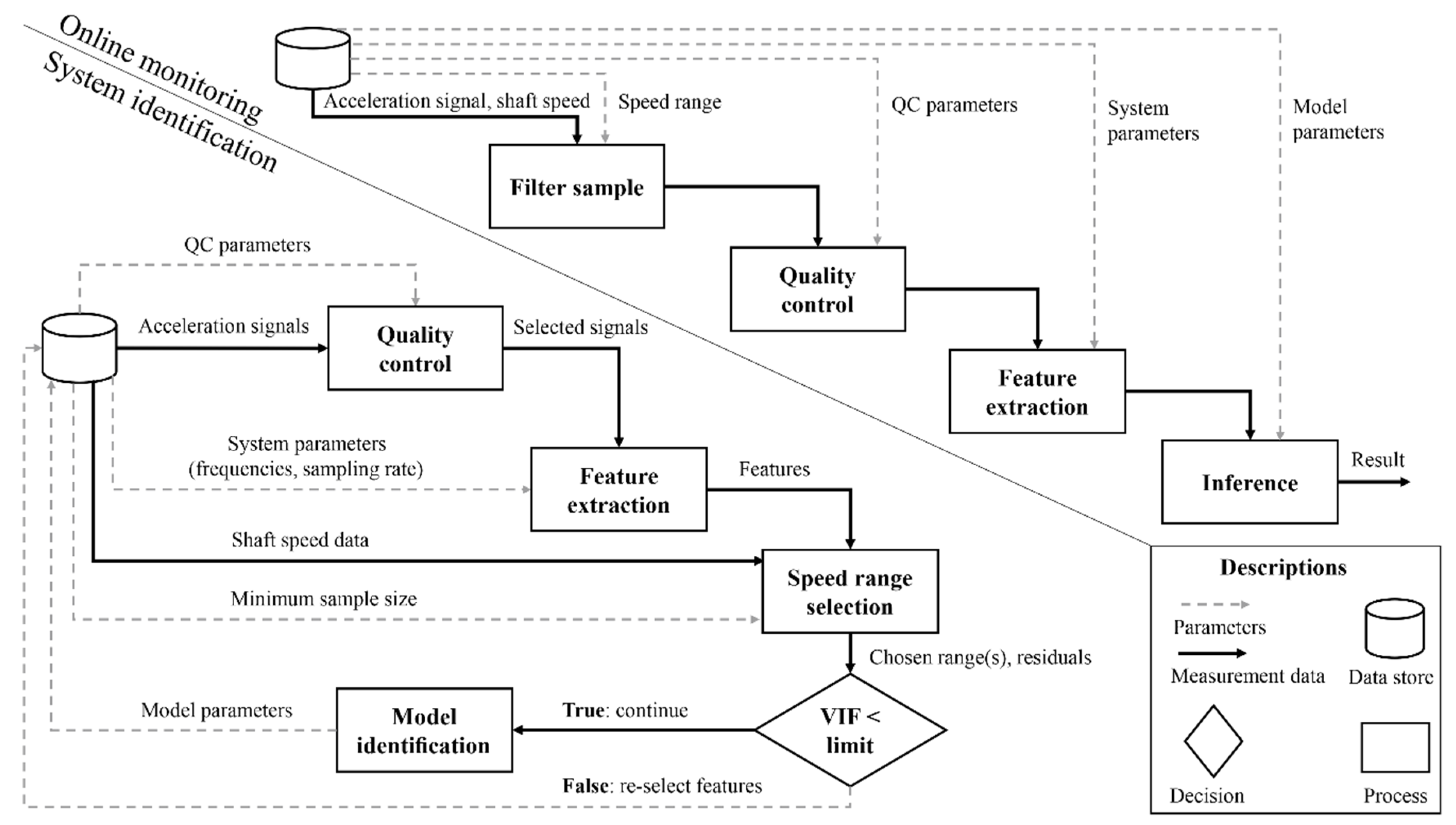
2.2. Condition Monitoring Algorithm
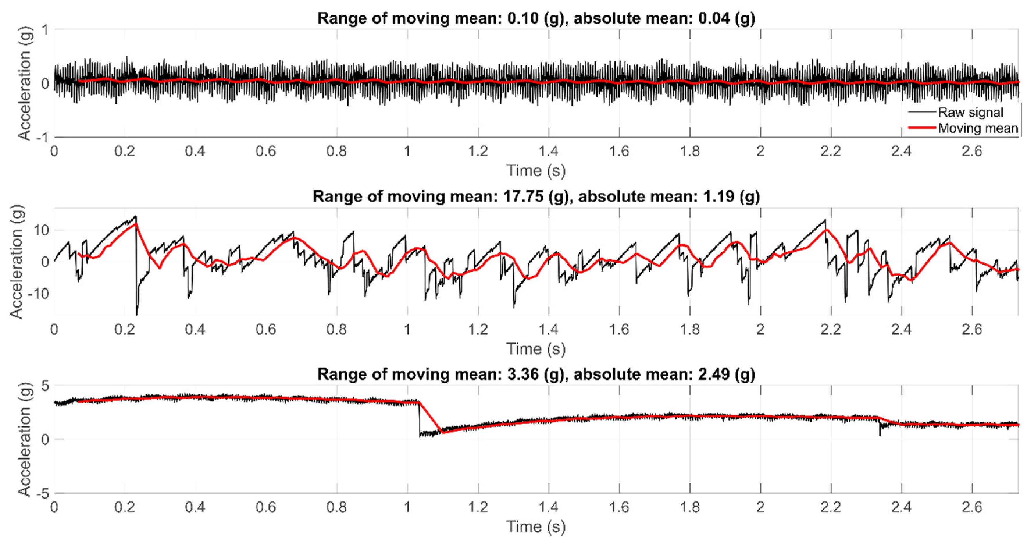
2.2.1. Data Quality Control
- The range of moving average of the acceleration signal is greater than a predefined limit.
- The acceleration values are constant.
- The absolute mean of the acceleration signal is greater than a predefined limit.
2.2.2. Feature Extraction
2.2.3. Residual Calculation
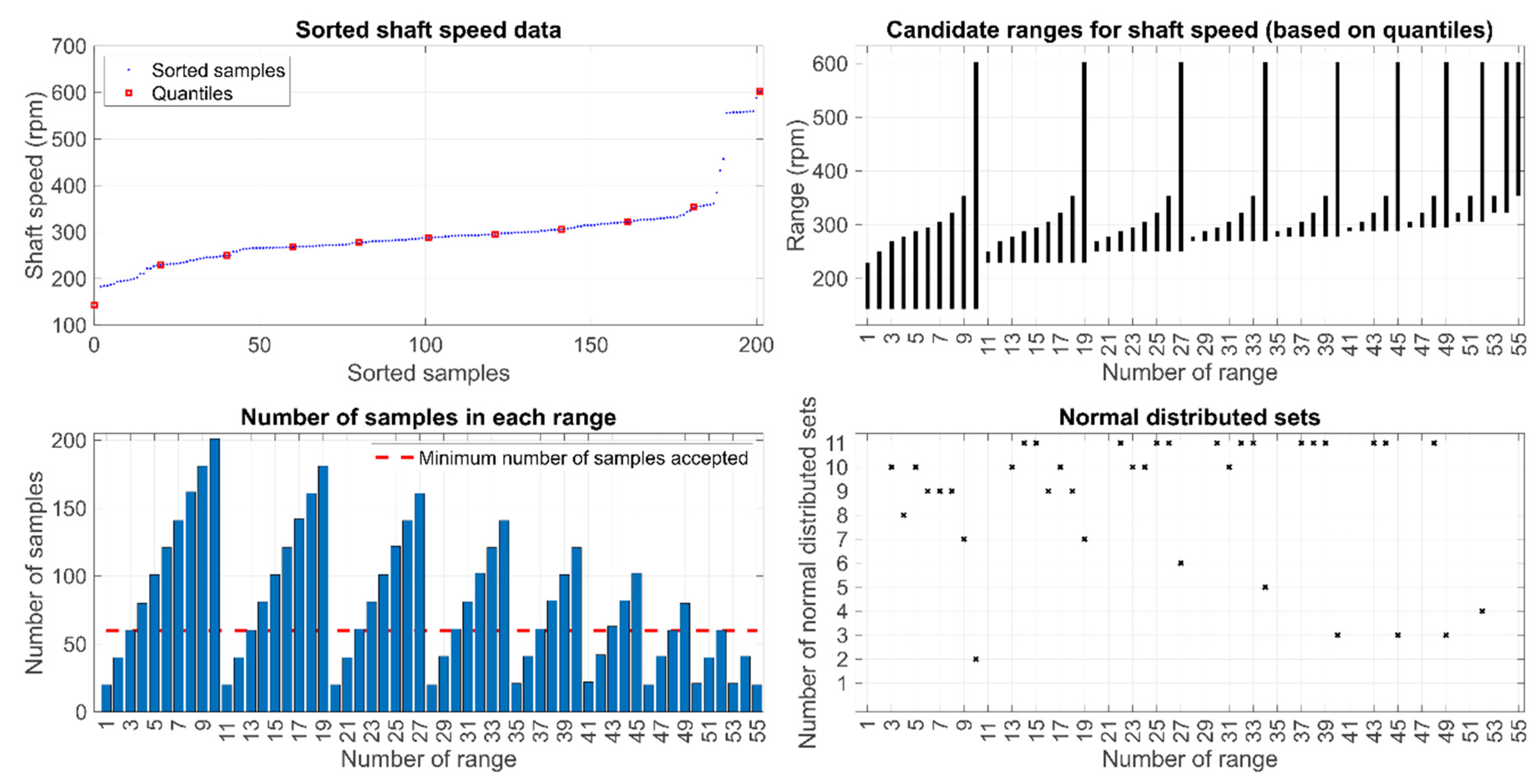
2.2.4. Shaft Speed Selection
2.2.5. Multicollinearity Check
2.2.6. Multivariate Normal Distribution
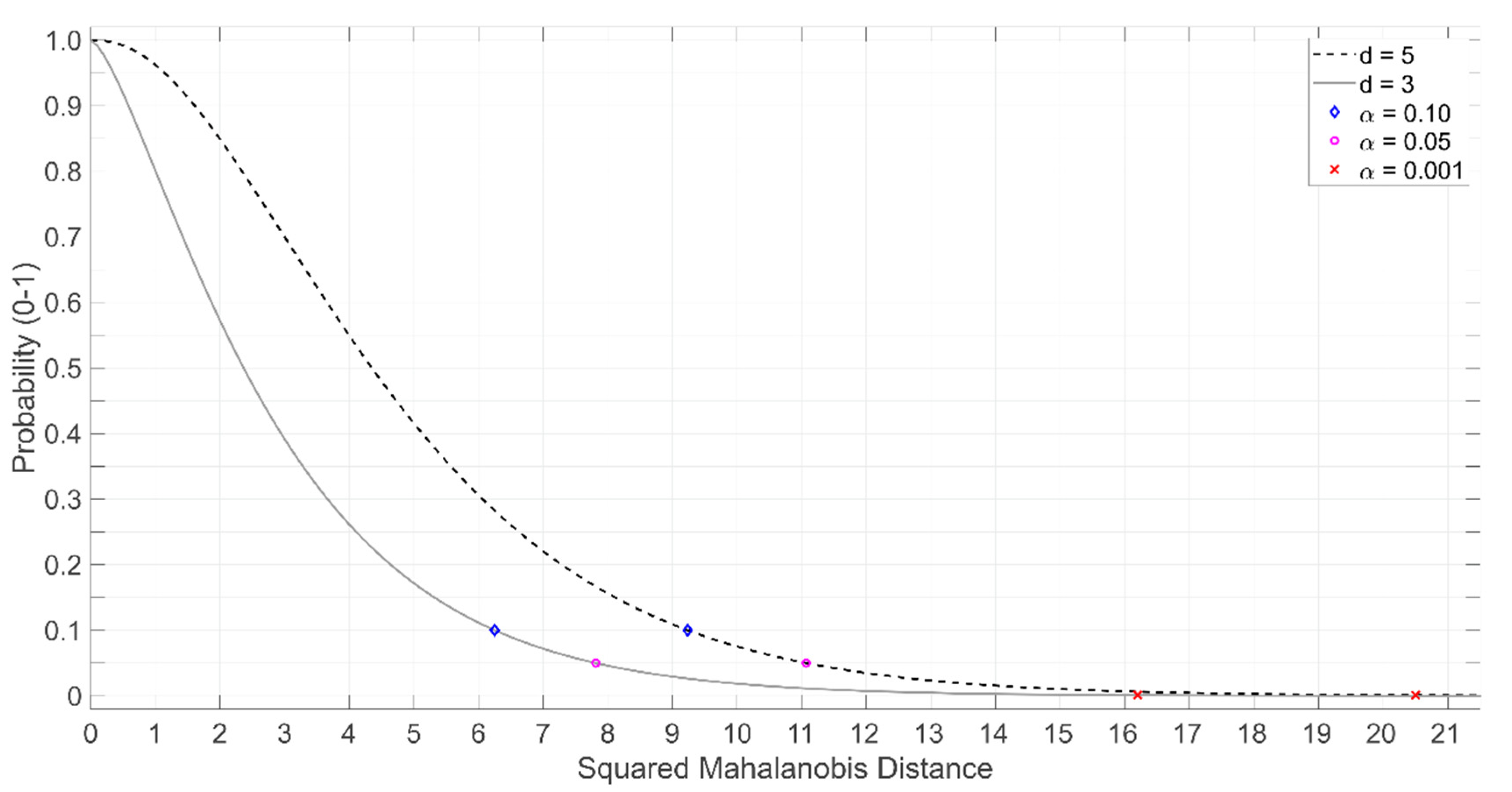
2.2.7. Probabilistic Monitoring
2.3. Classification Tests
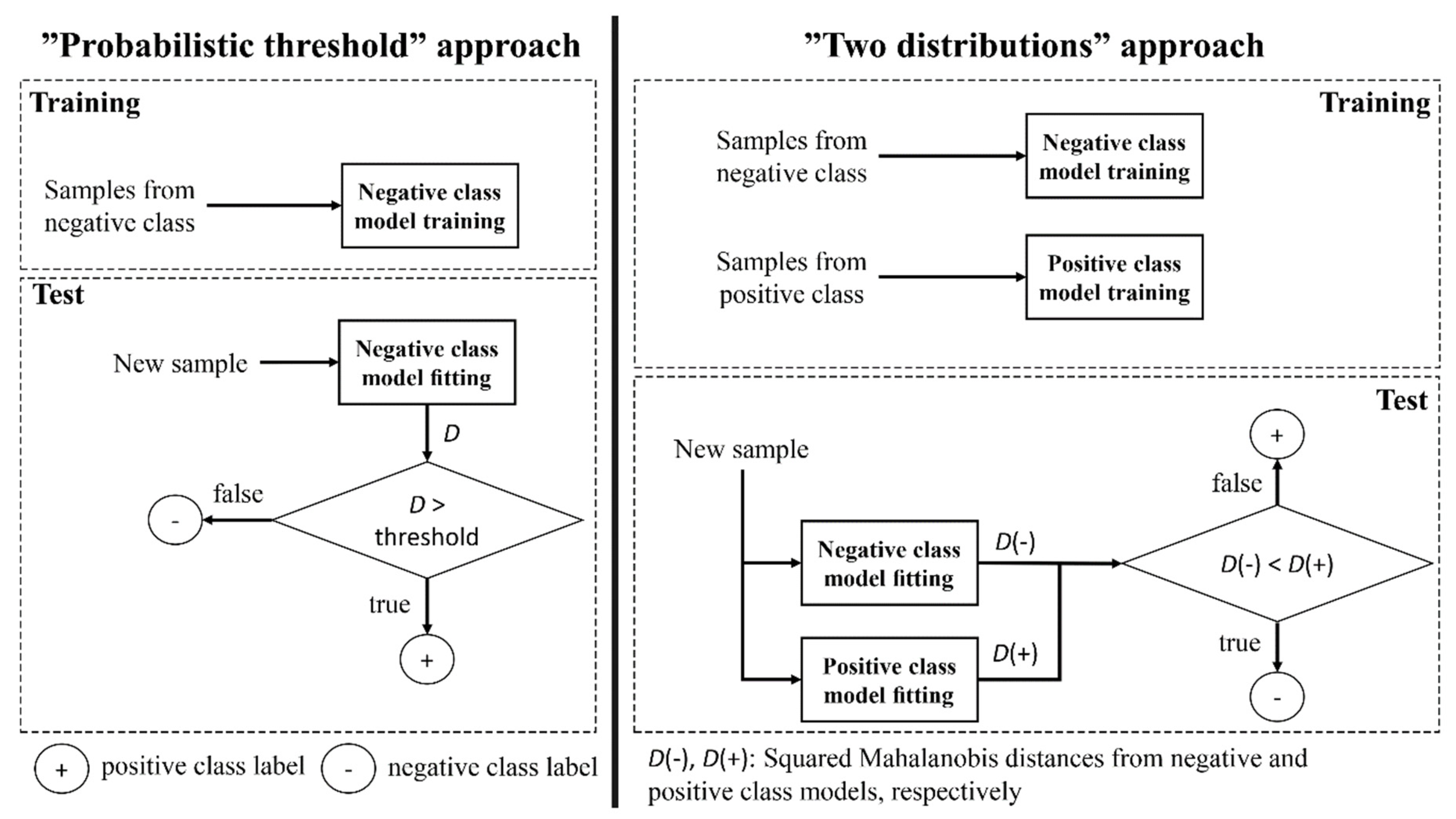
2.3.1. Classification Approaches for the Proposed Method
2.3.2. Reference Methods
2.3.3. Evaluation Criteria
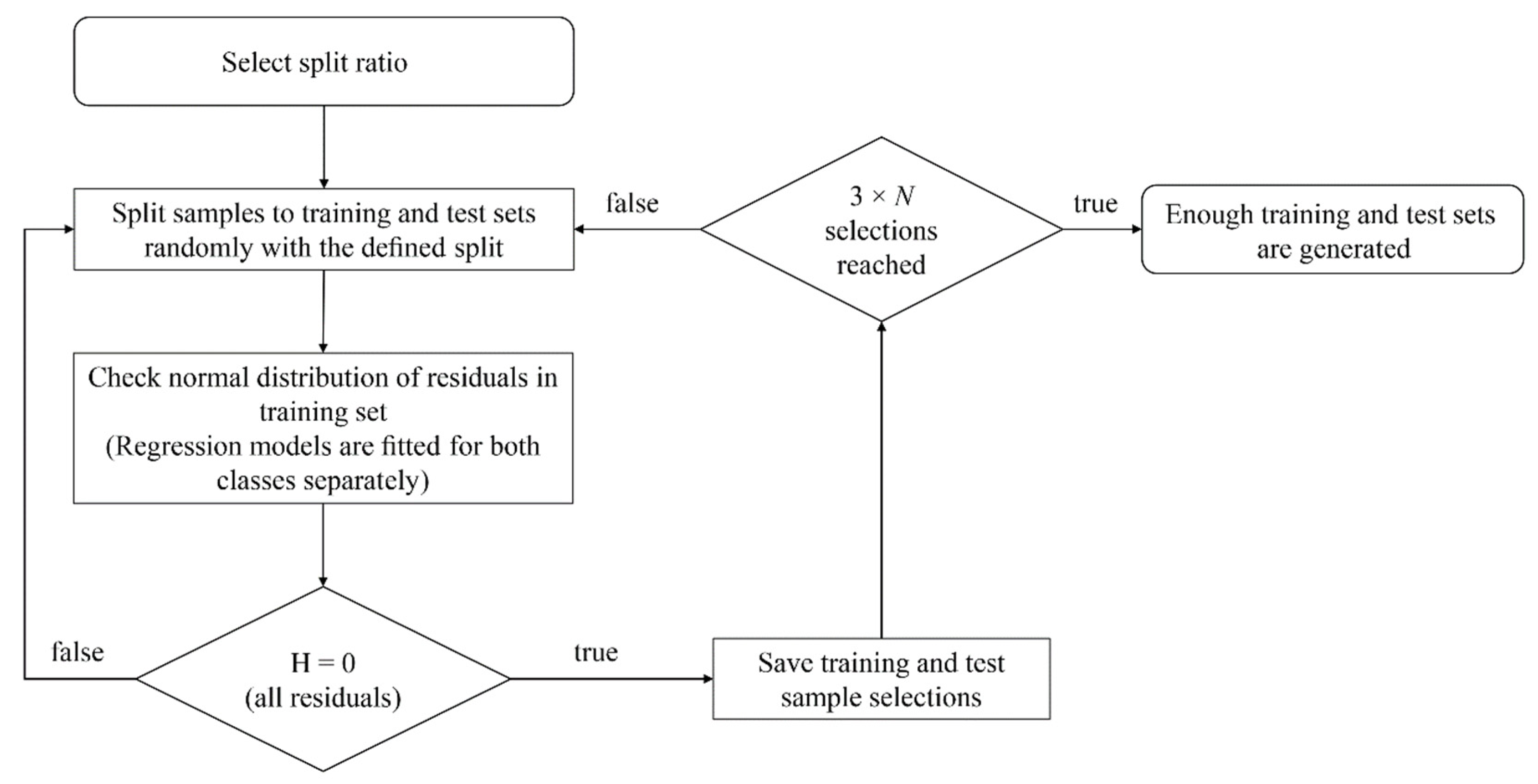
2.3.4. Nested Cross-Validation
3. Results and Discussion
3.1. Application on Data Sets
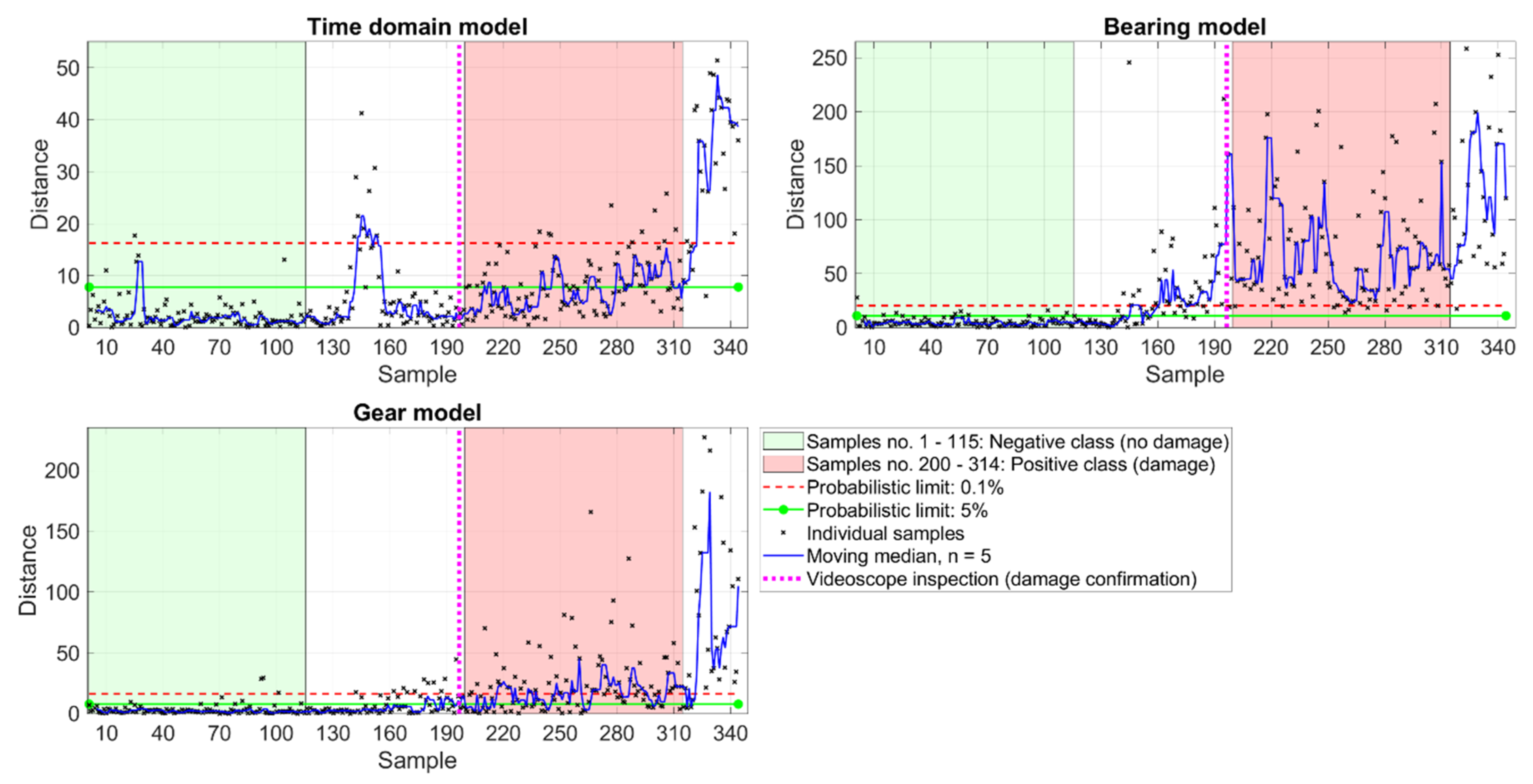
3.1.1. Thruster 1
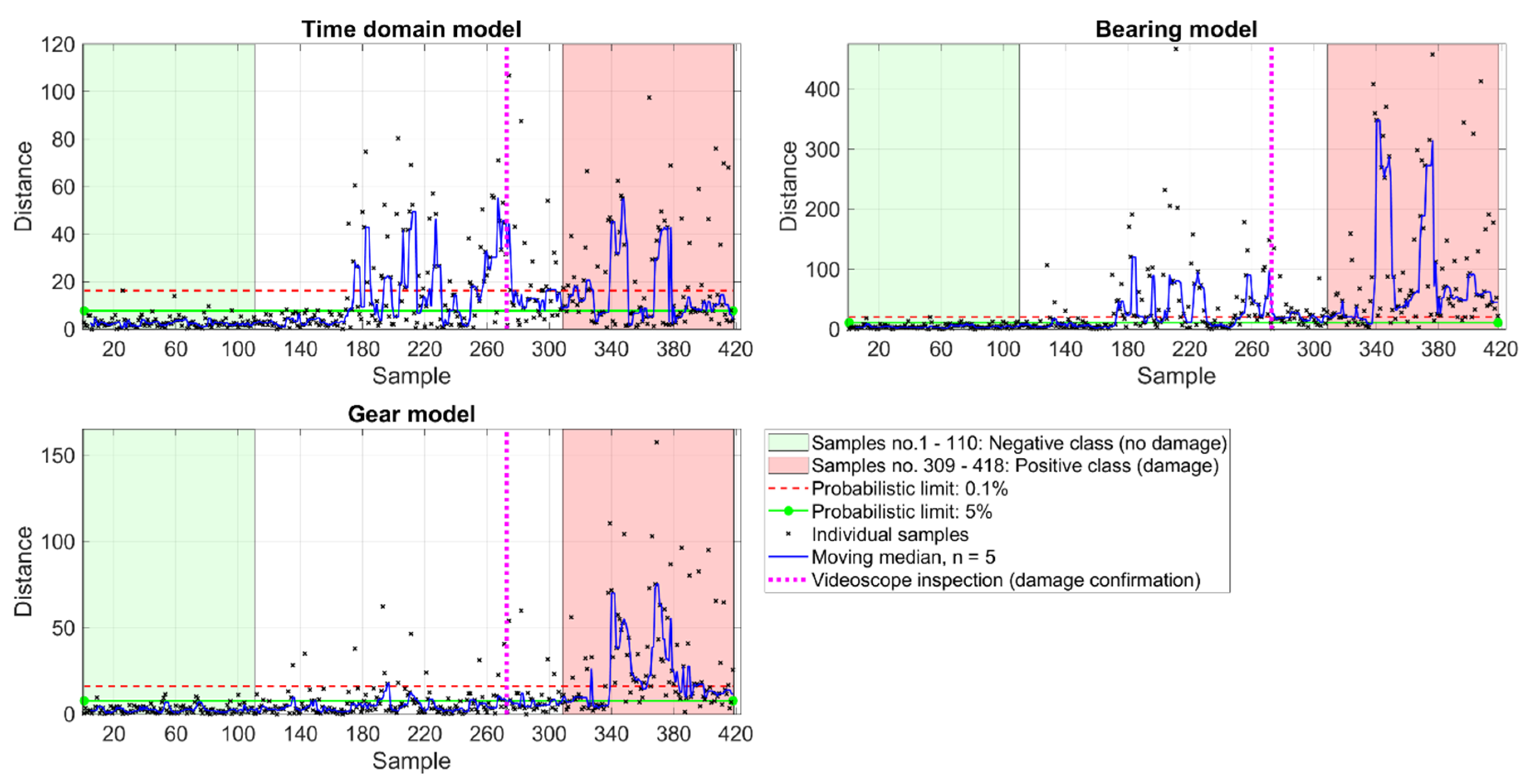
3.1.2. Thruster 2
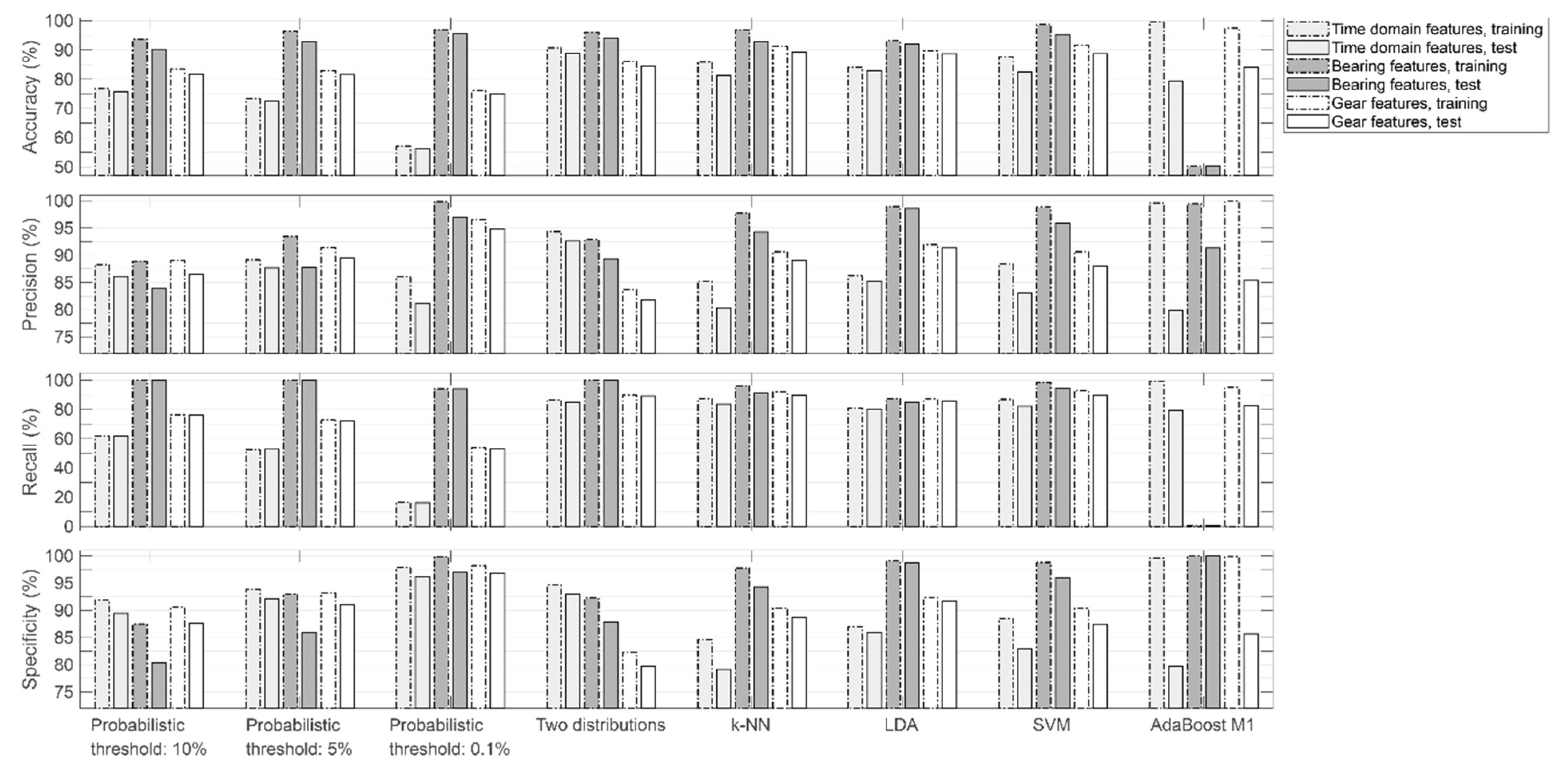
3.2. Classification Tests
3.3. Discussion
3.3.1. Significance of Results
3.3.2. Suggestions for Future Research
4. Conclusions
Author Contributions
Funding
Institutional Review Board Statement
Informed Consent Statement
Data Availability Statement
Acknowledgments
Conflicts of Interest
Appendix A

| Feature No. | σ | β0 | β1 | VIF |
|---|---|---|---|---|
| 1 | 9.09 × 10⁻³ | −30.42 × 10⁻³ | 415.16 × 10⁻⁶ | 1.15 |
| 2 | 194.62 × 10⁻³ | 2.53 | 228.01 × 10⁻⁶ | 1.81 |
| 3 | 171.79 × 10⁻³ | 3.38 | −1.04 × 10⁻³ | 1.62 |
| 4 | 236.88 × 10⁻⁶ | −2.00 × 10⁻³ | 9.95 × 10⁻⁶ | 1.15 |
| 5 | 231.94 × 10⁻⁶ | −256.99 × 10⁻⁶ | 3.44 × 10⁻⁶ | 1.09 |
| 6 | 88.18 × 10⁻⁶ | −725.54 × 10⁻⁶ | 3.55 × 10⁻⁶ | 1.04 |
| 7 | 153.40 × 10⁻⁶ | −2.04 × 10⁻³ | 9.99 × 10⁻⁶ | 1.11 |
| 8 | 55.34 × 10⁻⁶ | −811.19 × 10⁻⁶ | 3.61 × 10⁻⁶ | 1.03 |
| 9 | 94.55 × 10⁻⁶ | −714.60 × 10⁻⁶ | 4.29 × 10⁻⁶ | 1.55 |
| 10 | 71.53 × 10⁻⁶ | −498.69 × 10⁻⁶ | 2.44 × 10⁻⁶ | 1.02 |
| 11 | 140.14 × 10⁻⁶ | −240.91 × 10⁻⁶ | 2.43 × 10⁻⁶ | 1.55 |
| Feature No. | σ | β0 | β1 | VIF |
|---|---|---|---|---|
| 1 | 35.39 × 10⁻³ | −637.20 × 10⁻³ | 2.26 × 10⁻³ | 1.09 |
| 2 | 164.37 × 10⁻³ | 2.32 | 315.05 × 10⁻⁶ | 2.71 |
| 3 | 164.33 × 10⁻³ | 2.85 | 141.03 × 10⁻⁶ | 2.59 |
| 4 | 2.07 × 10⁻³ | −18.38 × 10⁻³ | 59.99 × 10⁻⁶ | 1.57 |
| 5 | 282.56 × 10⁻⁶ | −3.64 × 10⁻³ | 13.26 × 10⁻⁶ | 1.10 |
| 6 | 180.64 × 10⁻⁶ | −1.38 × 10⁻³ | 5.13 × 10⁻⁶ | 1.18 |
| 7 | 727.55 × 10⁻⁶ | −9.51 × 10⁻³ | 32.60 × 10⁻⁶ | 1.52 |
| 8 | 120.02 × 10⁻⁶ | −893.59 × 10⁻⁶ | 3.51 × 10⁻⁶ | 1.26 |
| 9 | 506.33 × 10⁻⁶ | −6.36 × 10⁻³ | 21.09 × 10⁻⁶ | 1.15 |
| 10 | 119.26 × 10⁻⁶ | −1.15 × 10⁻³ | 4.28 × 10⁻⁶ | 1.03 |
| 11 | 364.50 × 10⁻⁶ | −2.98 × 10⁻³ | 11.38 × 10⁻⁶ | 1.13 |
References
- Huang, Q.; Yan, X.; Zhang, C.; Zhu, H. Coupled transverse and torsional vibrations of the marine propeller shaft with multiple impact factors. Ocean Eng. 2019, 178, 48–58. [Google Scholar] [CrossRef]
- Fonte, M.; Reis, L.; Freitas, M. Failure analysis of a gear wheel of a marine azimuth thruster. Eng. Fail. Anal. 2011, 18, 1884–1888. [Google Scholar] [CrossRef]
- Henneberg, M.; Jorgensen, B.; Eriksen, R.L. Oil condition monitoring of gears onboard ships using a regression approach for multivariate T2 control charts. J. Process Control 2016, 46, 1–10. [Google Scholar] [CrossRef]
- Dang, J. DP Thrusters—Understanding Dynamic Loads and Preventing Mechanical Damages. In Proceedings of the Annual Conference of the Dynamic Positioning Committee, Houston, TX, USA, 14–15 October 2014. [Google Scholar]
- Boogaard, A.; Engels, E.; Wesselink, A. Health Monitoring of Steerable Thrusters. In Proceedings of the Annual Conference of the Dynamic Positioning Committee, Houston, TX, USA, 15–16 November 2005; pp. 825–844. [Google Scholar]
- Kambrath, J.K.; Yoon, C.; Mathew, J.; Liu, X.; Wang, Y.; Gajanayake, C.J.; Gupta, A.K.; Yoon, Y.-J. Mitigation of resonance vibration effects in marine propulsion. IEEE Trans. Ind. Electron. 2019, 66, 6159–6169. [Google Scholar] [CrossRef]
- Liu, Z.; Zhang, L. A review of failure modes, condition monitoring and fault diagnosis methods for large-scale wind turbine bearings. Measurement 2020, 149, 107002. [Google Scholar] [CrossRef]
- Sobie, C.; Freitas, C.; Nicolai, M. Simulation-driven machine learning: Bearing fault classification. Mech. Syst. Signal Process. 2018, 99, 403–419. [Google Scholar] [CrossRef]
- Zhang, S.; Zhang, S.; Wang, B.; Habetler, T.G. Deep learning algorithms for bearing fault diagnostics—A comprehensive review. IEEE Access 2020, 8, 29857–29881. [Google Scholar] [CrossRef]
- Lee, J.; Kao, H.-A.; Yang, S. Service innovation and smart analytics for Industry 4.0 and Big Data environment. Procedia CIRP 2014, 16, 3–8. [Google Scholar] [CrossRef] [Green Version]
- Diez-Olivan, A.; Del Ser, J.; Galar, D.; Sierra, B. Data fusion and machine learning for industrial prognosis: Trends and perspectives towards Industry 4.0. Inform. Fusion 2019, 50, 92–111. [Google Scholar] [CrossRef]
- Chen, J.; Li, J.; Chen, W.; Wang, Y.; Jiang, T. Anomaly detection for wind turbines based on the reconstruction of condition parameters using stacked denoising autoencoders. Renew. Energy 2020, 147, 1469–1480. [Google Scholar] [CrossRef]
- Zhang, Y.; Hutchinson, P.; Lieven, N.A.J.; Nunez-Yanez, J. Adaptive event-triggered anomaly detection in compressed vibration data. Mech. Syst. Signal Process. 2019, 122, 480–501. [Google Scholar] [CrossRef] [Green Version]
- Mahalanobis, P.C. On the generalised distance in statistics. Proc. Natl. Inst. Sci. India 1936, 2, 49–55. [Google Scholar]
- Yu, J. Adaptive hidden Markov model-based online learning framework for bearing faulty detection and performance degradation monitoring. Mech. Syst. Signal Process. 2017, 83, 149–162. [Google Scholar] [CrossRef]
- Castellani, F.; Garibaldi, L.; Daga, A.P.; Astolfi, D.; Natili, F. Diagnosis of Faulty Wind Turbine Bearings Using Tower Vibration Measurements. Energies 2020, 13, 1474. [Google Scholar] [CrossRef] [Green Version]
- De la Hermosa González-Carrato, R. Wind farm monitoring using Mahalanobis distance and fuzzy clustering. Renew. Energy 2018, 123, 526–540. [Google Scholar] [CrossRef]
- Jin, X.; Wang, Y.; Chow, T.W.S.; Sun, Y. MD-based approaches for system health monitoring: A review. IET Sci. Meas. Technol. 2017, 11, 371–379. [Google Scholar] [CrossRef]
- Sarmadi, H.; Karamodin, A. A novel anomaly detection method based on adaptive Mahalanobis-squared distance and one-class kNN rule for structural health monitoring under environmental effects. Mech. Syst. Signal Process. 2020, 140, 106495. [Google Scholar] [CrossRef]
- ISO. Condition Monitoring and Diagnostics of machines. Vibration Condition Monitoring. Part 3: Guidelines for Vibration Diagnosis; ISO 13373-3; SFS: Helsinki, Finland, 2015. [Google Scholar]
- Rai, A.; Upadhyay, S.H. A review on signal processing techniques utilized in the fault diagnosis of rolling element bearings. Tribol. Int. 2016, 96, 289–306. [Google Scholar] [CrossRef]
- Caesarendra, W.; Tjahjowidodo, T. A Review of Feature Extraction Methods in Vibration-Based Condition Monitoring and Its Application for Degradation Trend Estimation of Low-Speed Slew Bearing. Machines 2017, 5, 21. [Google Scholar] [CrossRef]
- Sharma, V.; Parey, A. A review of gear fault diagnosis using various condition indicators. Procedia Eng. 2016, 144, 253–263. [Google Scholar] [CrossRef] [Green Version]
- Lahdelma, S.; Juuso, E.K. Signal processing and feature extraction by using real order derivatives and generalised norms, Part 2: Applications. Int. J. Cond. Monit. 2011, 1, 54–66. [Google Scholar] [CrossRef]
- Ericsson, S.; Grip, N.; Johansson, E.; Persson, L.-E.; Sjöberg, R.; Strömberg, J.-O. Towards automatic detection of local bearing defects in rotating machines. Mech. Syst. Signal Process. 2005, 19, 509–535. [Google Scholar] [CrossRef] [Green Version]
- Janssens, O.; Slavkovikj, V.; Vervisch, B.; Stockman, K.; Loccufier, M.; Verstockt, S.; Van de Walle, R.; Van Hoecke, S. Convolutional neural network based fault detection for rotating machinery. J. Sound Vib. 2016, 377, 331–345. [Google Scholar] [CrossRef]
- Antoniadis, I.; Glossiotis, G. Cyclostationary analysis of rolling-element bearing vibration signals. J. Sound Vib. 2001, 248, 829–845. [Google Scholar] [CrossRef] [Green Version]
- Abboud, D.; Elbadaoui, M.; Smith, W.A.; Randall, R.B. Advanced bearing diagnostics: A comparative study of two powerful approaches. Mech. Syst. Signal Process. 2019, 114, 604–627. [Google Scholar] [CrossRef]
- Lahdelma, S.; Juuso, E.; Strackeljan, J. Neue Entwicklungen auf dem Gebiet der Wälzlagerüberwachung. In Proceedings of the Tagungsband zum 6. Aachener Kolloquium für instandhaltung, Diagnose und Anlagenüberwachung, AKIDA 2006, Aachen, Germany, 14–15 November 2006; pp. 447–460. [Google Scholar]
- Feng, Z.; Liang, M.; Chu, F. Recent advances in time-frequency analysis methods for machinery fault diagnosis: A review with application examples. Mech. Syst. Signal Process. 2013, 38, 165–205. [Google Scholar] [CrossRef]
- Randall, R.B.; Antoni, J. Rolling element bearing diagnostics—A tutorial. Mech. Syst. Signal Process. 2011, 25, 485–520. [Google Scholar] [CrossRef]
- Guyon, I.; Elisseeff, A. An introduction to variable and feature selection. J. Mach. Learn. Res. 2003, 3, 1157–1182. [Google Scholar]
- Nikula, R.-P.; Karioja, K.; Pylvänäinen, M.; Leiviskä, K. Automation of low-speed bearing fault diagnosis based on autocorrelation of time domain features. Mech. Syst. Signal Process. 2020, 138, 106572. [Google Scholar] [CrossRef]
- Kim, H.-E.; Tan, A.C.C.; Mathew, J.; Choi, B.-K. Bearing fault prognosis based on health state probability estimation. Expert Syst. Appl. 2012, 39, 5200–5213. [Google Scholar] [CrossRef]
- Bakdi, A.; Kouadri, A.; Mekhilef, S. A data-driven algorithm for online detection of component and system faults in modern wind turbines at different operating zones. Renew. Sustain. Energy Rev. 2019, 103, 546–555. [Google Scholar] [CrossRef]
- May, R.; Dandy, G.; Maier, H. Review of input variable selection methods for artificial neural networks. In Artificial Neural Networks—Methodological Advances and Biomedical Applications; Suzuki, K., Ed.; IntechOpen: Rijeka, Croatia, 2011; pp. 19–44. [Google Scholar]
- James, G.; Witten, D.; Hastie, T.; Tibshirani, R. An Introduction to Statistical Learning with Applications in R; Springer: New York, NY, USA, 2013. [Google Scholar]
- Lahdelma, S.; Juuso, E.K. Signal Processing in Vibration Analysis. In Proceedings of the Fifth International Conference on Condition Monitoring and Machine Failure Prevention Technologies, Edinburgh, UK, 15–18 July 2008; pp. 867–878. [Google Scholar]
- McFadden, P.D.; Smith, J.D. Vibration monitoring of rolling element bearings by the high-frequency resonance technique—A review. Tribol. Int. 1984, 17, 3–10. [Google Scholar] [CrossRef]
- Smith, W.A.; Borghesani, P.; Ni, Q.; Wang, K.; Peng, Z. Optimal demodulation-band selection for envelope-based diagnostics: A comparative study of traditional and novel tools. Mech. Syst. Signal Process. 2019, 134, 106303. [Google Scholar] [CrossRef]
- Massey, F.J. The Kolmogorov-Smirnov test for goodness of fit. J. Am. Stat. Assoc. 1951, 46, 68–78. [Google Scholar] [CrossRef]
- Anderson, T.W.; Darling, D.A. Asymptotic theory of certain “goodness-of-fit” criteria based on stochastic processes. Ann. Math. Statist. 1952, 23, 193–212. [Google Scholar] [CrossRef]
- Bender, R.; Lange, S. Adjusting for multiple testing—When and how? J. Clin. Epidemiol. 2001, 54, 343–349. [Google Scholar] [CrossRef]
- Manly, B.F.J.; Navarro Alberto, J.A. Multivariate Statistical Methods: A Primer, 4th ed.; CRC Press: Boca Raton, FL, USA, 2017. [Google Scholar]
- Etherington, T.R. Mahalanobis distances and ecological niche modelling: Correcting a chi-squared probability error. PeerJ 2019, 7, e6678. [Google Scholar] [CrossRef] [PubMed]
- Aggarwal, C.C. Outlier analysis. In Data Mining; Springer: Cham, Switzerland, 2015; pp. 237–263. [Google Scholar]
- Baraldi, P.; Cannarile, F.; Di Maio, F.; Zio, E. Hierarchical k-nearest neighbours classification and binary differential evolution for fault diagnostics of automotive bearings operating under variable conditions. Eng. Appl. Artif. Intell. 2016, 56, 1–13. [Google Scholar] [CrossRef] [Green Version]
- Daga, A.P.; Fasana, A.; Marchesiello, S.; Garibaldi, L. The politecnico di torino rolling bearing test rig: Description and analysis of open access data. Mech. Syst. Signal Process. 2019, 120, 252–273. [Google Scholar] [CrossRef]
- Gryllias, K.C.; Antoniadis, I.A. A Support Vector Machine approach based on physical model training for rolling element bearing fault detection in industrial environments. Eng. Appl. Artif. Intell. 2012, 25, 326–344. [Google Scholar] [CrossRef]
- Li, Y.; Cal, Y.-Z.; Yin, R.-P.; Xu, X.M. Fault Diagnosis based on Support Vector Machine Ensemble. In Proceedings of the Fourth International Conference on Machine Learning and Cybernetics, Guangzhou, China, 18–21 August 2005; pp. 3309–3314. [Google Scholar]
- Shao, J. Linear model selection by cross-validation. J. Am. Stat. Assoc. 1993, 88, 486–494. [Google Scholar] [CrossRef]
- Baumann, K. Cross-validation as the objective function for variable-selection techniques. Trac-Trend. Anal. Chem. 2003, 22, 395–406. [Google Scholar] [CrossRef]
- Oakland, J.S.; Followell, R.F. Statistical Process Control, a Practical Guide, 2nd ed.; Heinemann Newnes: Oxford, UK, 1990. [Google Scholar]
- Dunson, D.B. Statistics in the big data era: Failures of the machine. Stat. Probab. Lett. 2018, 136, 4–9. [Google Scholar] [CrossRef]
- Beleites, C.; Neugebauer, U.; Bocklitz, T.; Krafft, C.; Popp, J. Sample size planning for classification models. Anal. Chim. Acta 2013, 760, 25–33. [Google Scholar] [CrossRef] [Green Version]
- Kadlec, P.; Grbic, R.; Gabrys, B. Review of adaptation mechanisms for data-driven soft sensors. Comput. Chem. Eng. 2011, 35, 1–24. [Google Scholar] [CrossRef]


| BPFI | BPFO | BSF | FTF | GMF |
|---|---|---|---|---|
| 10.8435 | 8.1565 | 3.3667 | 0.4293 | 13 |
| Process | Parameter(s) | Example Value |
|---|---|---|
| Quality control (QC parameters) | range limit (g), (1 g ≈ 9.81 m/s2) | 0.5 |
| absolute mean limit (g) | 2 | |
| Feature extraction (System parameters) | kinematic frequencies | - |
| sampling rate | - | |
| Inference (Model parameters) | α: probabilistic threshold | 0.001 |
| n: moving window size | 5 | |
| β0, β1, μ, σ, Σ: regression models, normal distributions | - | |
| Speed range selection | minimum sample size | 60 |
| Filter sample | speed range | - |
| No. | Feature | Details |
|---|---|---|
| 1 | Generalized norm (l10) | Order of norm, p = 10 |
| 2 | Ratio of norms (l20/l2) | Ratio of high-order norm (p = 20) to low-order norm (p = 2) |
| 3 | Kurtosis | Indicator for the tails of probability distribution |
| 4 | BPFI feature | Median amplitude of 1–10 BPFI harmonics |
| 5 | BPFO feature | Median amplitude of 1–10 BPFO harmonics |
| 6 | BSF feature | Median amplitude of {1, 2, 4, 6} BSF harmonics |
| 7 | BPFI sideband feature | Median amplitude of the nearest sidebands on both sides of BPFI harmonics (20 sidebands altogether, spaced at shaft rotational frequency) |
| 8 | BSF sideband feature | Median amplitude of the nearest sidebands on both sides of BSF harmonics (8 sidebands altogether, spaced at FTF) |
| 9 | GMF feature 1 | Median amplitude of 1–4 GMF harmonics and two nearest sidebands on both sides (20 frequency components altogether) |
| 10 | GMF feature 2 | Median amplitude of 1 × GMF and two nearest sidebands on both sides (5 frequency components altogether) |
| 11 | GMF feature 3 | Median amplitude of 2 × GMF and two nearest sidebands on both sides (5 frequency components altogether) |
| No. | 1 | 2 | 3 | 4 | 5 | 6 | 7 | 8 | 9 | 10 | 11 |
|---|---|---|---|---|---|---|---|---|---|---|---|
| Features | 0.75 | 0.08 | −0.14 | 0.69 | 0.32 | 0.67 | 0.83 | 0.83 | 0.71 | 0.61 | 0.36 |
| Residuals | 0 | 0 | 0 | 0 | 0 | 0 | 0 | 0 | 0 | 0 | 0 |
| Parameters | Definition | Number of Parameters |
|---|---|---|
| β0, β1 | Regression parameters for each feature | 22 |
| μ | Means of each residual set (≈0) | 11 |
| σ | Standard deviations of each residual set | 11 |
| Σ1, Σ2, Σ3 | Covariance matrices | 3 |
| Classifier | Hyperparameter Values | Matlab® Function |
|---|---|---|
| k-NN | ‘NumNeighbors’: 1–49, odd numbers only | fitcknn |
| LDA | ‘Gamma’: 0–1, step 0.025 ‘Delta’: 0 and 1 × 10−6 × 10x, where x = 0–9, step 1 | fitcdiscr |
| SVM | ‘KernelScale’: 1 × 10−5 × 10x, where x = 0–10, step 0.4 ‘BoxConstraint’: 1 × 10−5 × 10x, where x = 0–10, step 0.4 | fitcsvm |
| AdaBoost M1 | ‘LearnRate’: {0.1, 0.25, 0.5, 0.75, 1} ‘MaxNumSplits’: 10–90, step 10 ‘NumLearningCyles’: 10–150, step 20 | fitcensemble |
Publisher’s Note: MDPI stays neutral with regard to jurisdictional claims in published maps and institutional affiliations. |
© 2021 by the authors. Licensee MDPI, Basel, Switzerland. This article is an open access article distributed under the terms and conditions of the Creative Commons Attribution (CC BY) license (http://creativecommons.org/licenses/by/4.0/).
Share and Cite
Nikula, R.-P.; Ruusunen, M.; Keski-Rahkonen, J.; Saarinen, L.; Fagerholm, F. Probabilistic Condition Monitoring of Azimuth Thrusters Based on Acceleration Measurements. Machines 2021, 9, 39. https://0-doi-org.brum.beds.ac.uk/10.3390/machines9020039
Nikula R-P, Ruusunen M, Keski-Rahkonen J, Saarinen L, Fagerholm F. Probabilistic Condition Monitoring of Azimuth Thrusters Based on Acceleration Measurements. Machines. 2021; 9(2):39. https://0-doi-org.brum.beds.ac.uk/10.3390/machines9020039
Chicago/Turabian StyleNikula, Riku-Pekka, Mika Ruusunen, Joni Keski-Rahkonen, Lars Saarinen, and Fredrik Fagerholm. 2021. "Probabilistic Condition Monitoring of Azimuth Thrusters Based on Acceleration Measurements" Machines 9, no. 2: 39. https://0-doi-org.brum.beds.ac.uk/10.3390/machines9020039