1. Introduction
Over the last decades, automotive original equipment manufacturers (OEM) aimed to make their cars increasingly smarter, more autonomous, and safer by widening the use of efficient electronic control units (ECUs) and active systems to improve both vehicle performance and passengers’ safety. Since the anti-lock braking system (ABS) was introduced for serial production, several advanced driver-assistance systems (ADASs) have been developed for vehicle longitudinal, lateral, and vertical stability control [
1,
2,
3]. As a result, modern cars, even those belonging to the city car segment, feature a plethora of ADAS functions. Besides the older longitudinal dynamics controllers, such as the ABS [
4], the adaptive cruise control (ACC) [
5], and the traction control system (TCS) [
6,
7,
8,
9], other functionalities recently arose targeting the lateral stability enhancement, such as the electronic stability program (ESP) [
10,
11], the active front steering (AFS) [
12,
13,
14] and the direct yaw moment controller (DYC) for torque vectoring (TV) transmission control [
15]. Even if less common than the former systems, vertical dynamics control systems, such as the active suspension control (ASC) [
16] and the active body control (ABC) [
17], are being introduced in top-end passenger cars to improve safety and ride comfort. As a result, the complexity of modern vehicle control systems is reaching hardly sustainable levels, with up to over 100 million lines of source code distributed on board among over 100 ECUs [
18].
ADASs generally improve vehicle safety and stability, but their effectiveness relies on the accurate estimation of the instantaneous vehicle dynamic states [
19], enabled by a variety of onboard sensors, such as inertial navigation sensors (INS), global navigation satellite systems (GNSS), and wheel speed and orientation sensors [
20,
21]. Besides estimation, ADASs rely on model predictive control strategies to correctly perform their safety actions, thus requiring the embedding of a numerical vehicle dynamic (VD) model on the ECU.
In the literature, different dynamic models and formulations estimate vehicle performance in terms of longitudinal, vertical, and lateral dynamics. Advanced simulations delivering high-accuracy predictions rely on high-fidelity rigid multibody (MB) models [
22,
23], which can be eventually enriched by vehicle body concept models to account for the body flexibility as well [
24,
25]. However, the MB modelling approach is quite complex and demands high computational effort. It may lead to MB models with more than 100 bodies, each of which needs an accurate definition of constraints, geometry, and mass properties. Although new efficient ECUs have been developed and recent studies tried to achieve real-time (RT) MB simulation of vehicle dynamics in embedded applications [
26,
27,
28], the computation is often too expensive with respect to the limited amount of computational resources of an embedded platform, and it is not always compatible with hard RT constraints.
The use of concept models, consisting of lumped-parameter models commonly used during the early-stage design phases, emerged for targeting RT embedded applications. Concept models represent a computationally more affordable alternative to the corresponding high-fidelity MB models, enabling an accurate and reliable RT prediction of the vehicle dynamic behaviour as required by ADASs [
29]. The lumped-parameter vehicle models (LPVMs) consist of a few bodies and a limited number of degrees of freedom (DOFs) with associated relatively low computational cost. Their complexity ranges from simple 2 DOF quarter-car or bicycle models, which can capture only the basic vertical and either the longitudinal or the lateral behaviour of a vehicle, up to 15–18 DOF full-vehicle models (FVMs) [
30,
31,
32]. Offering a good compromise between predictive accuracy and computational efficiency, FVMs already proved their effectiveness in supporting the vehicle dynamic simulation for RT driver-in-the-loop (DiL) testing [
33,
34]. A human driver immersed into a virtual-reality scenario acts on a virtual vehicle, enabling the assessment both subjectively and objectively of the influence of multiple design choices related, but not limited to, VD performances. Furthermore, FVMs are also enabling the development of more recent control strategies aiming for autonomous driving, such as fuzzy controllers [
35] and/or proportional–integral–derivative (PID) controllers [
36,
37].
This work’s contribution builds on the verge of extending the above-mentioned DiL approach, including some of the more basic autonomous driving functions, such as steering and throttle control, leading to the concept of virtual-driver-in-the-loop (vDiL) simulations. The proposed vDiL approach enables comparative vehicle design assessments on different driving scenarios while achieving a more objective benchmark than the human driver-in-the-Loop (hDiL) alternative. In practice, a replica of the virtual driver program is used in different simulations, while varying the design parameters under investigation.
In particular, this paper describes the main components and the overall architecture of a simulation environment required to evaluate the vehicle dynamic performances using vDiL. The presented simulation environment enables the validation of the vDiL results, while investigating more complex scenarios where the impact of the ADAS or even of the autonomous driving functions can be assessed [
38,
39].
The presented research originates from the need for simulating several independently controlled actors, while allowing to choose among several vehicle variants, with different types of models or different control strategies. This motivation led us to design a new simulation environment, which was deeply inspired from a predecessor simulator [
34]. The new architecture relies on the benefits of the object-oriented programming paradigm and exploits a hierarchical evaluation of the vehicle sub-modules, which is also more representative of the hierarchical organization of the plethora of different ECUs used in modern cars.
Within the proposed simulation framework and for the sake of describing a first proof-of-concept validation, we adopted a 14 DOF FVM that exchanges information with scalable-detail models of the remaining core vehicle sub-systems such as tyre, engine, and steering system. Moreover, a vDiL agent module was programmed. In particular, our testing scenarios exemplify how the proposed simulation platform enabled the comparison of the lateral dynamics of two vehicles with identical physical characteristics, but with two different strategies for driving torque distribution, i.e., a simplified mechanical differential model [
40,
41] and a DYC-based torque vectoring (TV) system [
42].
The paper is organized as follows.
Section 2 describes the concurrent software architecture of the simulator.
Section 3 explains the implemented driving tests.
Section 4 discusses the computational efficiency of the proposed simulator and presents the achieved level of concurrency. Moreover, it discusses the numerical results achieved during constant steer (CS) and constant radius (CR) tests according to ISO 4138, along with a severe lane change (SLC) manoeuvre as defined by ISO 3888 standard.
Section 5 provides concluding remarks and an overview of future developments.
2. Architecture of the Simulation Environment
A new simulation environment was designed and implemented using modern C++ (ISO 17), although we were inspired by an existing simulator [
34]. Thanks to the modern object-oriented programming (OOP) paradigm, the proposed simulator offers a modular infrastructure, where code procedures and data are hierarchically grouped and systematically encapsulated into objects [
27]. This allows a more effective representation of the increasing level of complexity required from the vehicle industry market.
In fact, the OOP paradigm is based on the concept of “objects”, which can contain data, in the form of fields or attributes or properties, but also embed specific functionalities, in the form of procedures or methods able to process the known data and produce new objects. Exploiting OOP, the design of the environment was more natural, as it allowed to focus on expressing the interactions and hierarchies between objects, more than on the data transactions and the corresponding procedures typical of the older procedural programming approach. Moreover, we exploited polymorphism to effectively capture the modular but also hierarchical variety of objects necessary for the dynamic simulation of several variants of a vehicle. In fact, the proposed software architecture more naturally supports the implementation of a multitude of alternatives for each sub-component of the vehicle, while it captures the interfaces between them at a more abstract level. Thanks to OOP and modern C++ (ISO 17), the vehicle simulation manager class was programmed to be thread-safe: several variants of a vehicle can be simulated concurrently.
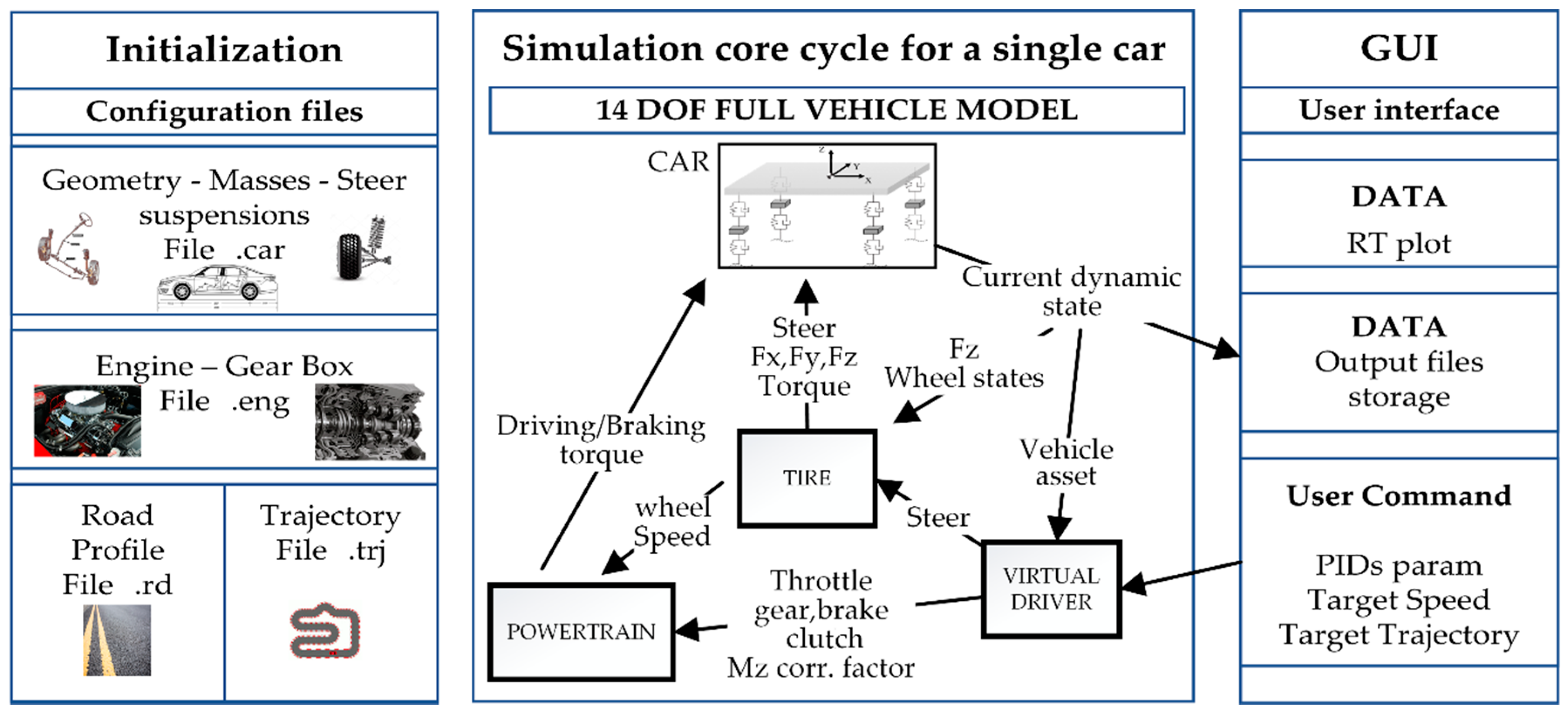
Figure 1 depicts the proposed modular architecture. The simulation starts by instantiating one or more vehicle objects. Each vehicle is created as an independent instance of the same abstract object class, which relies on several interacting sub-objects such as the car, tyre, powertrain, or driver sub-modules. Each vehicle instance retrieves the information required for its own construction, using a set of specific configuration files. Different configuration files define the required vehicle properties such as car geometry, inertial parameters, masses, steering system, engine, tyres, and suspension characteristics. Each of the input files must obey a prescribed syntax format, although OOP would also allow the easy implementation of the possibility of supporting different input file syntaxes.
The number and type of the input files depend on the type of object used to define the simulation: if the user sets a driving torque distribution strategy based on a DYC for TV, two more configuration files are required to provide the reference yaw rate lookup table (LUT) defined as explained in [
42].
At least two more additional configuration files are used to define road profiles and trajectories that vehicles must follow during the same prescribed ride simulation.
After the file-based initialization stage, the proposed simulation environment enables the concurrent simulation of different vehicles, each encapsulating its characteristics and control strategies. A dedicated graphical user interface (GUI) was instrumental for editing at runtime the different PID parameters, allowing for a better and more efficient fine-tuning of the dedicated PID-based virtual driver’s behaviour.
The RT vehicle simulations, in response to the virtual driver’s actions, are computed using a very efficient numerical model for vehicle dynamic simulation based on a lumped-parameter formulation with 14 DOFs. A set of output signals, such as car position, forces, and torques, are sent to the GUI enabling RT data visualization, in addition to their storage for post-processing purposes.
To prevent slowing down the simulation execution, the communication towards the GUI application was delegated within a lower-priority thread using a client–Server User Datagram Protocol (UDP).
The vehicle simulation is based on a modular architecture relying on four sub-moduels: car, powertrain, tyre, and virtual driver. Each of the sub-module classes was defined allowing its evaluation to run in a separated thread, with no dependencies either on the states of the other sub-modules or on the communication towards the external GUI. To prevent concurrency issues such as race condition and deadlock and achieve thread-safety, we used the shared-memory paradigm, enriched by the usage of a set of dedicated memory mutexes. All the above-mentioned concurrent programming features are supported natively by modern C++ since the 2011 revision, making the current version of the code immediately portable towards different platforms, including the embedded ones.
2.1. Car Sub-Module
The car sub-module represents the core of the system implementing the lumped-parameter FVM. It is an explicit solver for the set of ordinary differential equations (ODEs) governing the dynamic equilibrium of the vehicle chassis (three translational and three rotational equilibrium conditions) and of each of the wheels (translational equilibrium in the vertical direction and rotational equilibrium around the spindle axis). The 14 DOFs of the model are as follows:
the 3 rigid-body rotations (pitch, roll, and yaw) of the vehicle body;
the 3 rigid-body translations of the vehicle body;
the vertical displacement of each wheel centre w.r.t. to the vehicle body;
the rotation of each wheel around the spindle axis.
2.2. Powertrain Sub-Module
The powertrain sub-module is responsible for computing the angular velocity of the engine, from which the engine torque, T
d, is derived by interpolating the specified maximum torque–velocity curve and scaling it by the throttle command. The torque distribution to the driving wheels is considered even for a vehicle equipped with a conventional mechanical differential, while the following uneven distribution is implemented for a vehicle equipped with DYC for TV:
where T
rdw and T
ldw are the torque values delivered to the right and left wheel, respectively, while R
w is the wheel radius, d the vehicle half-track width, and M
z is the yaw moment required by the desired understeer correction calculated as described in [
43]. For the vehicles used in the proposed simulation, we used R
w = 0.3135 m and d = 1.4673 m.
2.3. Tyre Sub-Module
The tyre sub-model is responsible for simulating the road–tyre interaction and computing the vertical, longitudinal, and lateral forces, along with the longitudinal and lateral slip coefficients. At each simulation step, vertical forces are estimated by a simple spring–damper model. Longitudinal and lateral forces are computed using a simplified version of Pacejka Magic Formula, as explained in detail in [
41].
2.4. Virtual Driver
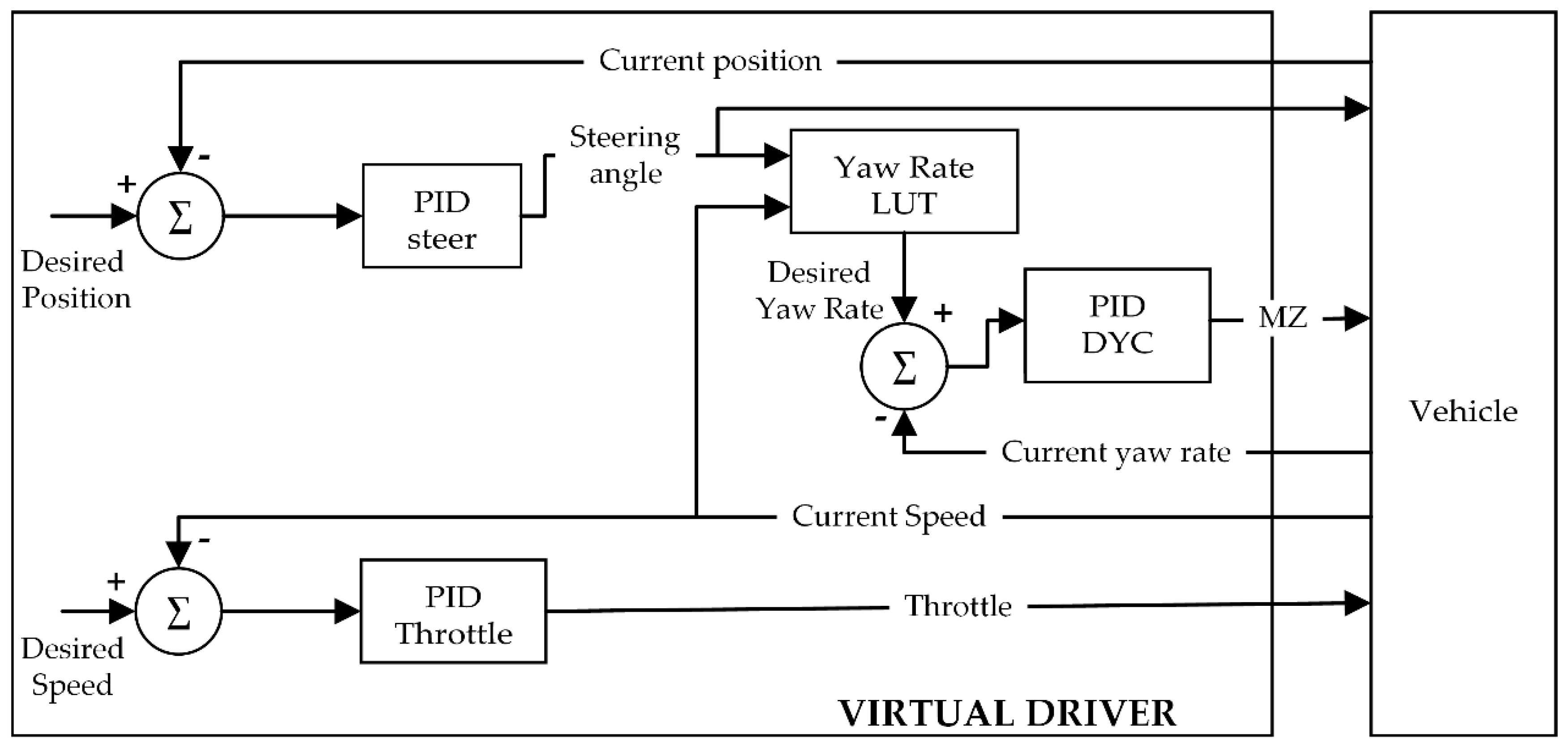
The driver sub-module of the simulation software is used to control the throttle position, the steering wheel angle, and the M
z correction factor using three nested PID regulators as described in [
40,
41] and depicted in
Figure 2. A kinematic model is implemented to derive the steering angle at wheels, based on the actual value of the steering input given by the virtual driver and on the steering ratio.
Three independent PID controllers are used to calculate the values of the steering wheel angle (δ), the throttle command (th), and, in the case of a vehicle with DYC, the desired yaw moment, Mz, input.
Considering the discrete-time nature of the simulation, all the implemented PID regulators rely on a classical formulation as follows:
where
is the current cross-track error determined as the distance of the current vehicle position from the reference trajectory;
represents the error between the target speed and the current vehicle speed; and
is the error between the current vehicle yaw rate and the desired yaw rate. The index, k, is the number of the current iteration timestep in a range from 1 to N, with N representing the total number of simulation timesteps. The integration time, dt, represents the time interval between two consecutive iteration steps. It is worth noting than the duration of dt has a remarkable influence on the overall quality and stability of simulation. On the one hand, an extremely low value of dt corresponds to a very dense time discretization, thus assuring a high dynamic accuracy of the simulation results. However, this can lead to numerical instabilities when using discrete derivatives, such as in Equations (3)–(5), in presence of numerical noise [
40]. On the other hand, higher values of dt generally reduce the dynamic accuracy, leading to information loss and potentially instability and divergency when simulating highly dynamic problems. In the scope of this paper, we used values of the integration time, dt, between 0.001 and 0.005 s, assuring a good compromise between accuracy and stability corresponding to these values. K
pδ, K
iδ, and K
dδ are the proportional, integral, and derivative gains, respectively, for the steer regulator; K
pth, K
ith, and K
dth are the proportional, integral, and derivative gains for the throttle regulator;
,
, and
are the proportional, integral, and derivative gains for the throttle regulator.
3. Virtual Driving Tests
Several driving tests were carried out based on ISO standard manoeuvres to assess the effectiveness of the implemented simulator. The most relevant tests carried out were those concerning the evaluation of lateral behaviour of the vehicles by simulating the CS, CR, and SLC manoeuvre.
The first two tests are defined by the ISO 4138 standard for the characterization of understeering characteristics of the vehicle, and the last one is defined by ISO 3888 standard. The ISO 4138 defines a standardization of the driving manoeuvres to evaluate the understeer gradient of a vehicle. It consists in varying a specific feature of the vehicle motion, while measuring and keeping constant other motion features.
Table 1 summarizes the constant, varied, and measured features for each of the two tests.
As explained in [
43], in dynamic conditions, the steering angle δ is given by
where L is the wheelbase length of the vehicle; R, the turning radius; and a
y, the lateral acceleration. The understeer gradient, K, can be derived as follows:
The lateral acceleration depends on the longitudinal velocity, s, and the turning radius, being
In real driving scenarios, vehicles are equipped with specific sensors to measure δ, s, and ay from which the understeer gradient, K, is derived, while in the virtual tests proposed in this work, those values are estimated by the implemented 14 DOF FVM.
CR and CS manoeuvres can be used alternatively, being the steady-state equilibrium independent of the actual testing method. The values of speed, steering wheel angle, or turning radius can be obtained holding constant any of the three, while varying the second in a controlled way and measuring the third one.
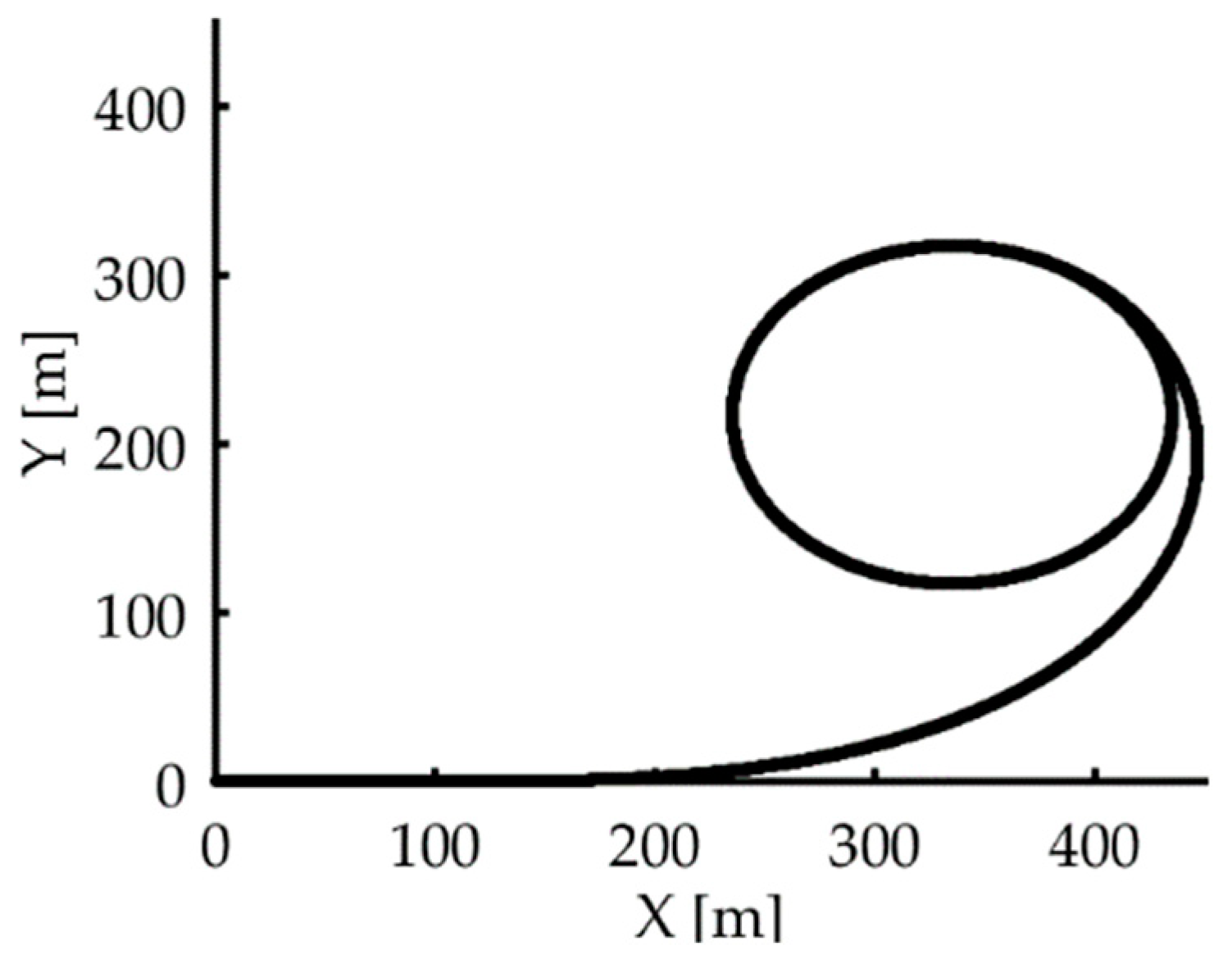
In the implemented CR manoeuvre, the two vehicles are driven by virtual PID-controlled drivers at different speeds along the trajectory shown in
Figure 3, consisting of a clothoid, along which the vehicles are accelerated until reaching a speed of 30 km/h, followed by a circular trajectory of standard constant radius, R, equal to 100 m. At that point, the steering angle is increased up to the value of the Ackerman angle, which is calculated, for the test vehicles with a wheelbase L = 2.73 m, as
Once the vehicles are on the circular path, the virtual drivers accelerate from 30 to 100 km/h following a stepwise constant law, with a step of 5 km/h, while ensuring that the lateral acceleration increases by a rate not exceeding 0.1 m/s2/s, as ISO 4138 suggests. At each step, the speed is kept constant to ensure that steady-state conditions are maintained for at least 3 s. The understeer gradient is then calculated using Equation (7).
In addition to the CR test, a CS manoeuvre is implemented as well, during which the steering wheel angle is kept fixed and equal to the Ackerman value δAck, and the speed, s, of the vehicles is steadily increased from 50 to 160 km/h, again with a step of 5 km/h. With the imposed steering wheel angle, as the longitudinal speed increases, the car travels along circular trajectories with decreasing or increasing radii for an oversteering and an understeering behaviour, respectively.
When the car reaches steady-state conditions for a given speed value, s, the actual turning radius is calculated as follows:
The understeer gradient, K, is finally derived from Equation (7).
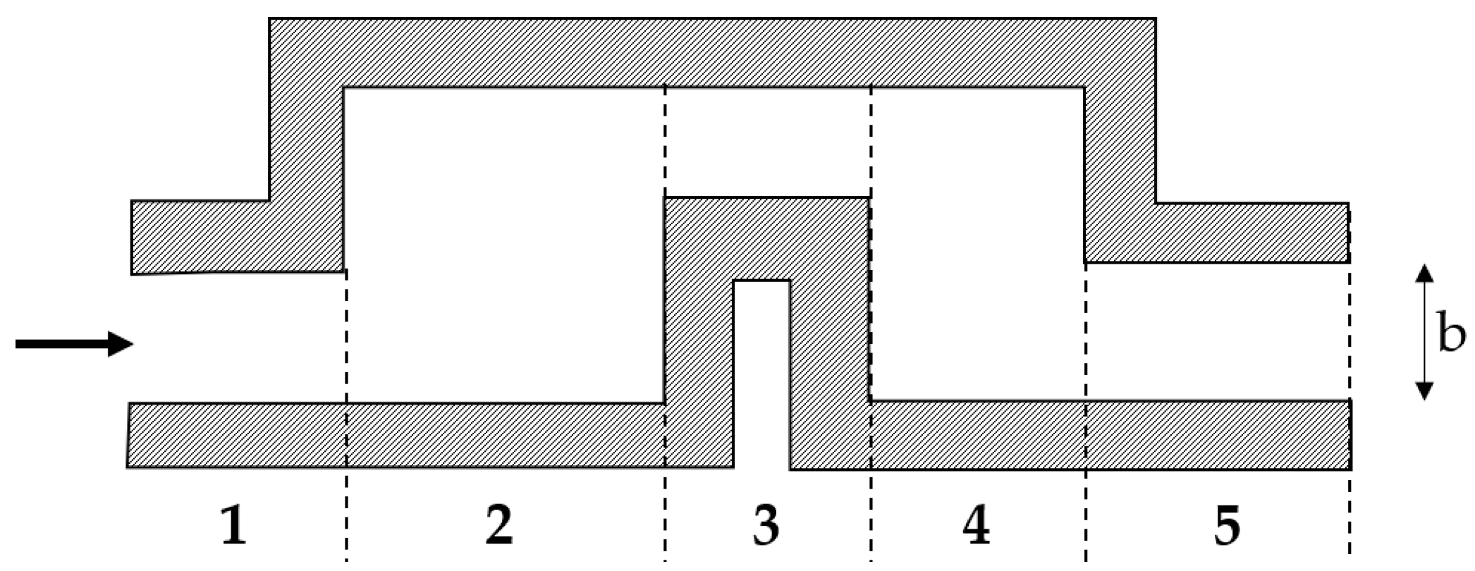
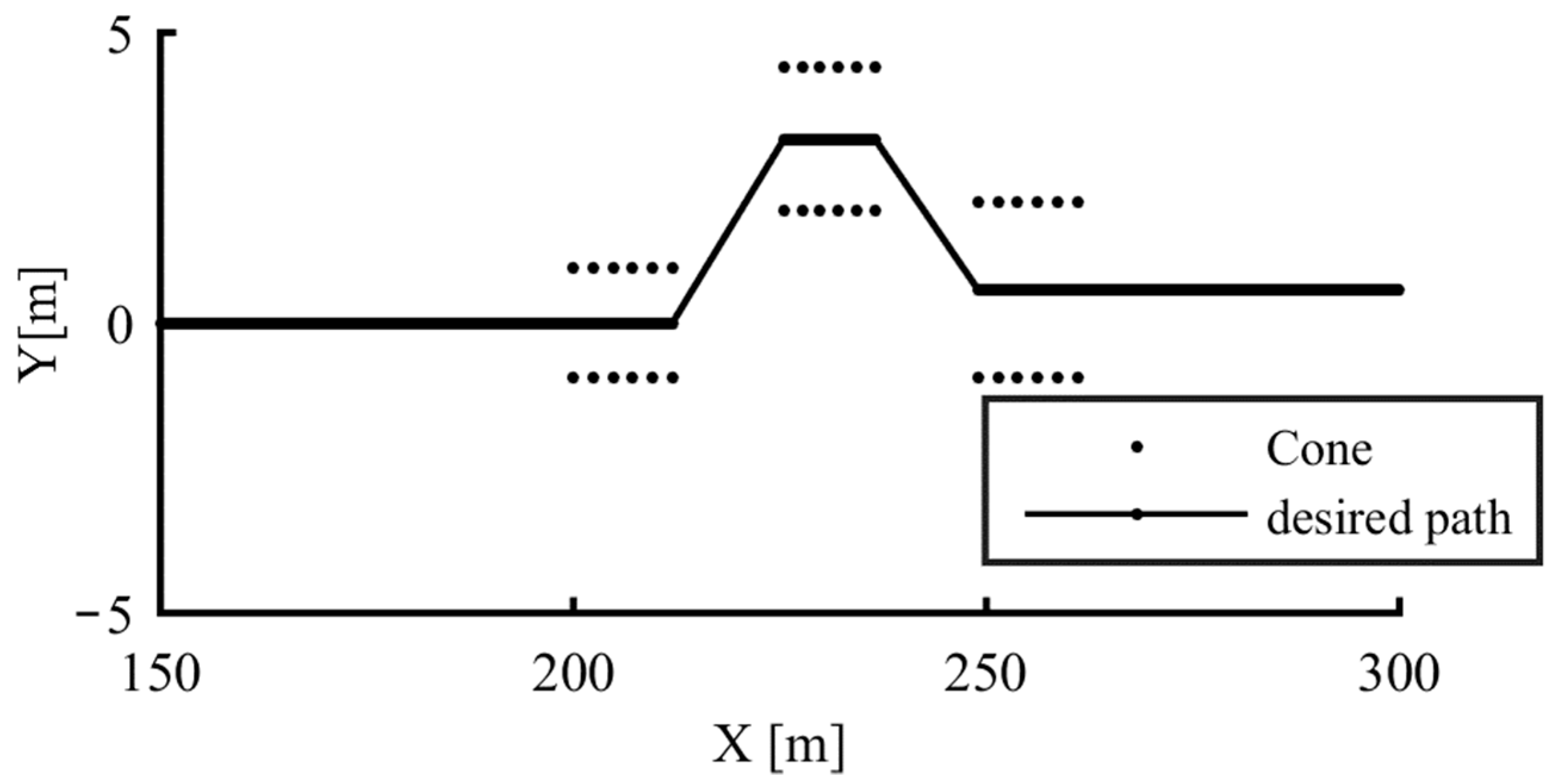
A third driving test has been implemented as well, consisting of an SLC manoeuvre defined according to the ISO 3888 standard. The latter defines the geometry of a test track, with a total length of 61 m, designed to enable the assessment of obstacle avoidance performance and road-holding capability of a vehicle. The test track, which is depicted in
Figure 4 and defined by the dimensional specifications listed in
Table 2, is marked by cones that are placed as shown in the schematic of
Figure 5.
To perform this manoeuvre, the virtual driver strives to follow as closely as possible the specific test trajectory that follows the middle line of the test track, as shown in
Figure 5.
In particular, the virtual vehicle is expected to enter
Section 1 with the highest gear position that allows guaranteeing a minimum engine speed of 2000 RPM during the manoeuvre, and after 2 m the driver must release the throttle and drive up to the end of
Section 5. The test is considered faultless if the vehicle never crosses the track borders as defined by the cones.
As explained in
Table 3, these manoeuvres must be executed using a different combination of the available PID regulators. To perform these tests at the same time, it is possible to instantiate several driver and vehicle objects with different characteristics. Specifically, three different drivers and two vehicles were instantiated. Each driver was assigned one of the above manoeuvres to be executed with two different vehicles. The following table shows the assigned manoeuvres and the activation status of the regulators for steer and throttle control in each test.
If the vehicle is configured to use the TV strategies, the DYC PID-controller is also activated in any of the three driver cases.
The two vehicles instantiated are identical, except for the driving torque distribution system: vehicle 1 is equipped with a simplified mechanical differential that performs an even torque distribution, while vehicle 2 exploits uneven driving torque distribution, controlled by a DYC approach. This further clarifies the advantages of OOP and the high flexibility of the proposed simulator that can simulate different driving scenarios concurrently. The advantages of concurrent simulation and the results of these driving tests are illustrated, respectively, in
Section 4.1 and
Section 4.2.
4. Results and Discussion
This section describes the numerical assessments conducted to highlight the benefits of the concurrent simulation architecture introduced using OOP (as discussed in
Section 2) and to validate the proposed vDiL approach’s usability. All results presented in this section have been achieved through simulations executed on a workstation featuring an Intel
® Core™ i7-6700HQ 2.60 GHz quad-core eight-thread processor, and 16 GB of DDR4 RAM, running on Windows 10 Enterprise operating system and assigning to the correspondent process higher execution priority. At first, tests assessed the level of concurrency with an increasing number of independent vehicles’ simulation. Afterwards, we demonstrated the potential of the platform and the presented virtual driver approach by simulating a set of comparative standard driving tests, which are typically adopted for performing vehicle dynamics objective evaluations on test tracks.
4.1. Assessment of the Concurrency Level
As described in
Section 2, this paper deals with the advantages of a concurrent simulation architecture, which allows multiple—and potentially although not necessarily different—car simulations to run concurrently.
In other words, the proposed concurrent software architecture is a necessary but not sufficient condition to achieve parallel RT execution of different car simulations. Concurrency refers just to the possibility of having various simulations to be launched independently. In contrast, achieving RT parallel simulation demands additional complexity levels: considering the time variable, mechanisms for enforcing time-related deadlines, and implementing dedicated constructs for coordinating and orchestrating the operations among all the parallel threads.
The proposed concurrent architecture can achieve real-time execution for all the simultaneously executed jobs provided that the available computing resources can meet the computational demands at any time. Therefore, it is interesting to consider a benchmark focusing on the scaling of the computational performances for an increasing number of concurrently simulated vehicles. Moreover, it not only allows the further evaluation of the efficiency of the proposed architecture but also assess the achieved level of concurrency.
We performed 10 different simulations with an increasing number of identical vehicles, during a path-following scenario. This context represents the more computationally demanding simulation case, because virtual drivers use all the regulators illustrated in
Figure 2.
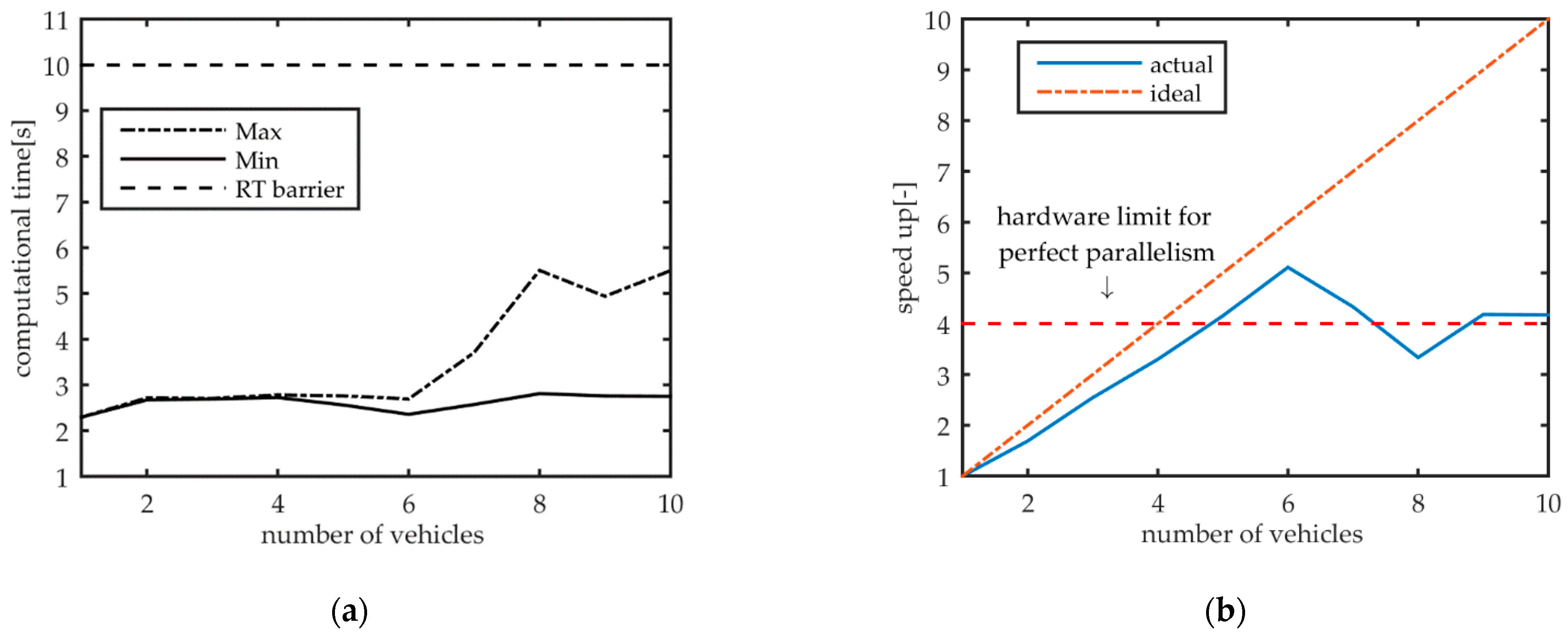
Figure 6a shows the trend of minimum and maximum computation times required when issuing an increasing number of parallel simulations. The almost constant value of the minimum curve tells us that there is always at least one thread, thus at least one parallel simulation, able to conclude the job with a performance comparable to the single-vehicle simulation case. Conversely, a sever degradation of the slowest thread performances happens only from above six concurrently simulated vehicles. This suggests that the computational resources within the used workstation are saturated only when we launch more than six concurrent threads: in all those cases, only a subset of the threads are able to stay resident on the CPU, while the remaining threads’ operations start to be scheduled asynchronously. Although the computational efficiency is out of the scope of this paper, it is worth noticing also that all the simulations were completed within the real-time barrier, showing great potential for achieving parallel real-time simulation of several vehicles.
Figure 6b depicts the results of the same benchmark, in terms of the achieved speed-up levels, computed as the ratio between the time required to complete all the simulations sequentially and the time required from the slowest thread simulation. This chart highlights more clearly that our architecture achieves almost perfect parallelism (slope of the blue curve is lower than that of the dash-dotted line) with a linear scaling up to 6 simulations. Above this value, the speed-up tends to saturate to a value of 4×, which indicates how our implementation can fully saturate all the CPU cores (dashed line). Fluctuations of the speed-up above 4× are achieved due to the Intel hyperthreading functionality, which allows the scheduling of the execution of more threads on the same physical core.
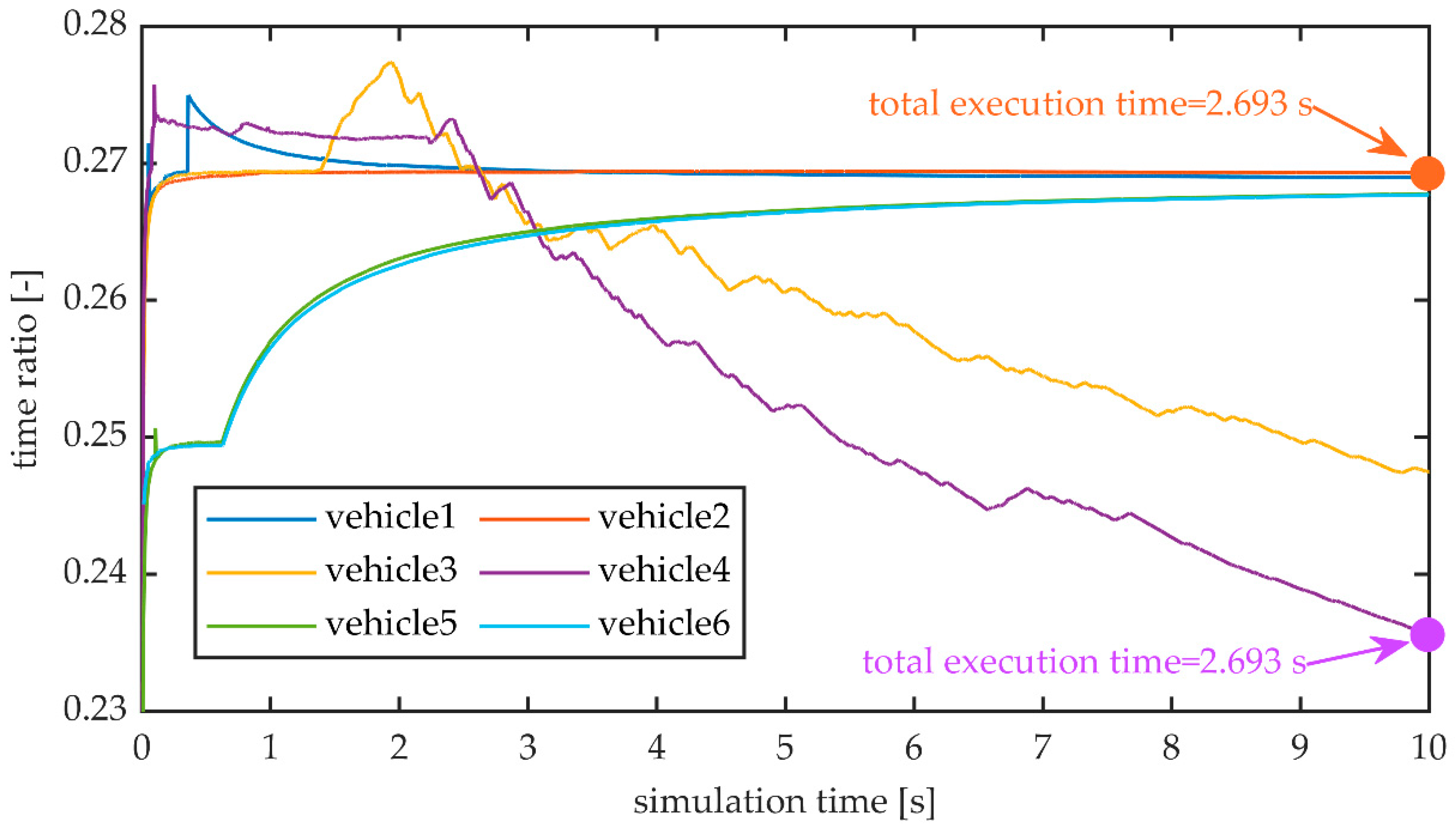
Figure 7 further clarifies the implication of concurrent execution of six identical vehicles, all performing the same CR driving test task for 10 s, showing the evolution of the time ratio between the software execution time, (t
exec), and the vehicle time, t
sim, calculated as follows:
As illustrated, the simulation of each vehicle is not synchronized with the simulation of the other vehicles, but it is performed asynchronously. The different simulations execute at a variable computing speed and the virtual vehicles are substantially free to race. It is worth mentioning that, with the simulations running on a pre-emptive multitasking operative system, with other programs running, the execution is not deterministic as it may be greatly influenced by several other factors suddenly changing the amount of available computing power, such as graphics drivers interrupts, other programs possibly running in the background, or system updates. At the very beginning, all the simulating threads are warming-up, which is consistent with the fact that the CPU frequency is rising and transitioning from lower energy-saving states to its maximum power. After few iterations, we can appreciate that vehicles 3 and 4 start being the slowest threads, but they were allocated more resources than the others, becoming the first two threads to complete. Similarly, simulations of vehicles 5 and 6 advanced with a degrading performance, asymptotically converging towards a time ratio threshold of about 0.27 s. As reported also in
Figure 6a, for the six simulations case, the total execution time ranged between 2.357 and 2.693 s, which is also reported at the rightmost side of the chart in
Figure 7. It is also worth noting that all the simulations were executed maintaining a large margin from the real-time barrier, corresponding to a time ratio equal to 1.
4.2. Results of the Virtual Driving Tests
This section illustrates an example of the simulation output for the CR, CS, and SLC driving tests. As mentioned in
Section 3, we used three drivers and two vehicles, with identical characteristics but with different torque distribution strategies. Each driver was assigned a specific manoeuvre, as indicated in
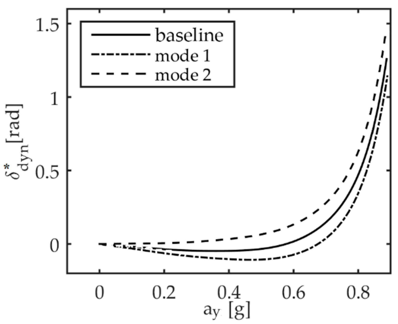
Table 3, to be done with the two different vehicles. In particular, vehicle 1 was supposed to be equipped with a simplified mechanical differential, providing an even torque distribution to the driving wheels. Vehicle 2 was designed to have a driving torque distribution based on two different TV strategies, to be used in two different driving modes. In the two modes, indicated as mode 1 and mode 2, the implemented TV-based DYC allows, respectively, to reduce and to increase the understeer gradient in comparison to vehicle 1 (corresponding to the baseline in
Figure 8).
Figure 8 shows the dynamic steering angle curve,
as a function of the lateral acceleration, a
y, for vehicle 1 (baseline) along with the desired curves for vehicle 2 (mode 1 and mode 2) when the vehicle speed is set to 25 m/s and a ramp signal is used to define the steering wheel input between 0° and 120° [
43]. Vehicle 1 shows an oversteering behaviour for lateral acceleration values up to 5.5 m/s
2. Thanks to DYC, vehicle 2 in mode 1 shows an oversteering behaviour up to 6.5 m/s
2 of lateral acceleration, while an understeering behaviour is achieved by vehicle 2 in mode 2 in the entire range of lateral acceleration.
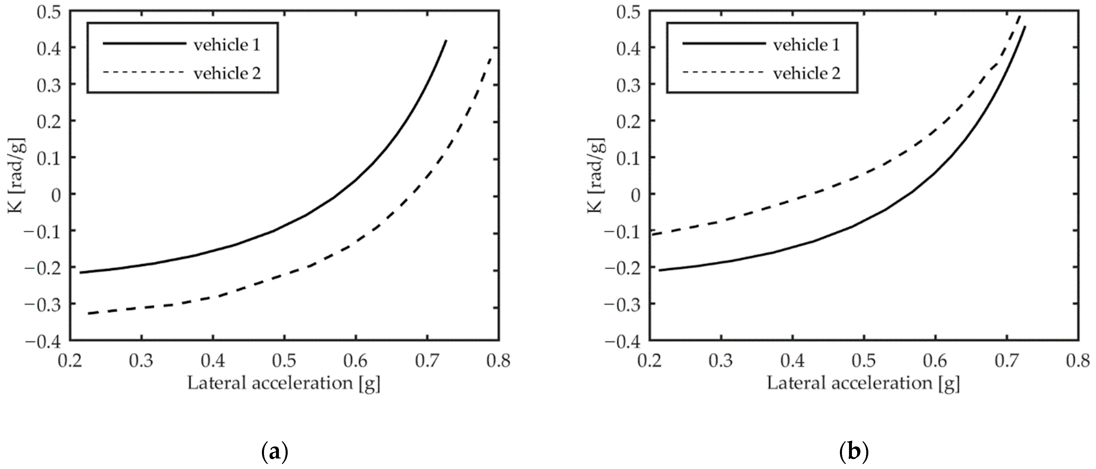
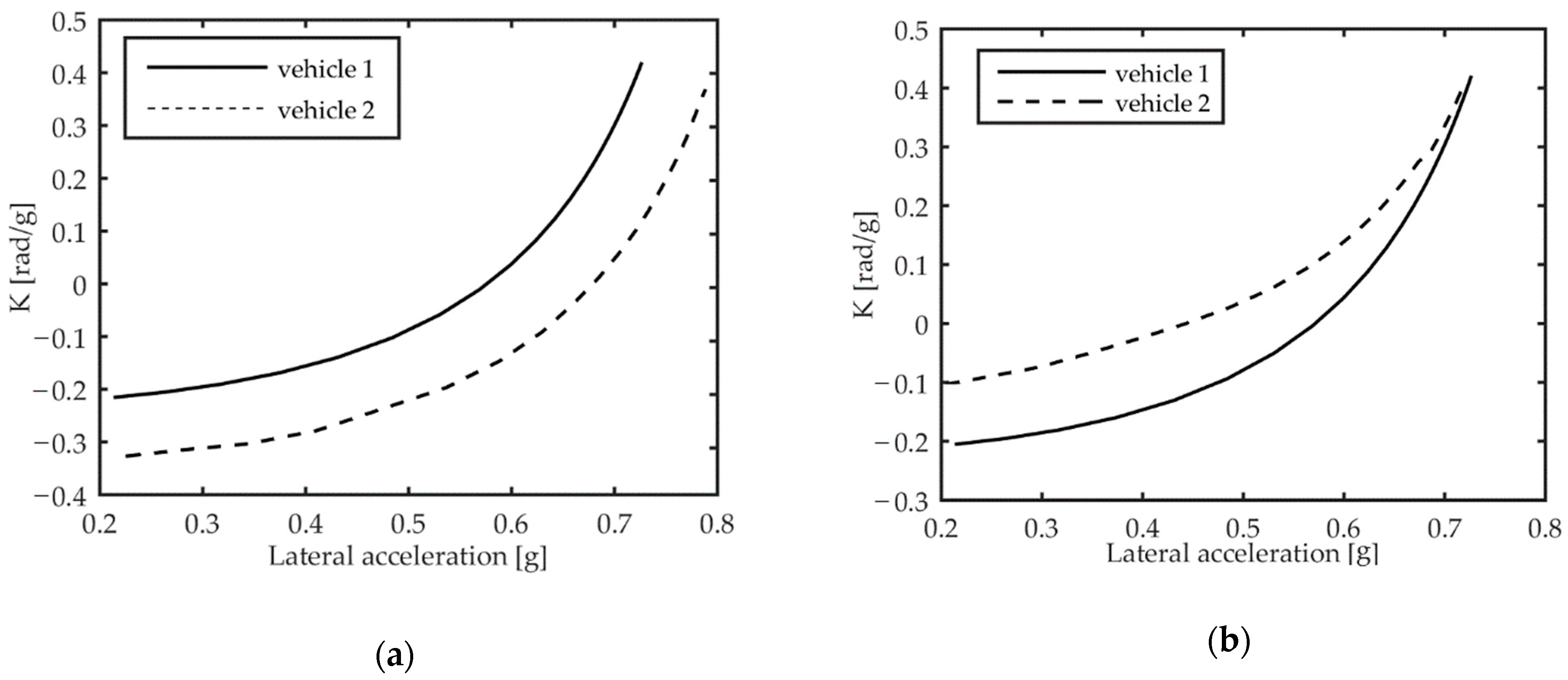
The implemented DYC allows following the desired
curve, for each driving mode of vehicle 2, with a maximum error of ±0.5°, as shown in
Figure 9 and
Figure 10, where the achieved trend of understeer gradient for vehicle 1 and vehicle 2 is calculated with the CR and CS tests, respectively.
As mentioned in the previous section, in steady-state conditions the two test methods are equivalent, as confirmed by the substantially identical results achieved in the simulated manoeuvres executed by driver 1 and driver 2.
As expected, using the driving mode 1 with driver 1, the understeer gradient of vehicle 2 is always lower than that of vehicle 1, while it is higher in driving mode 2 in the full range of lateral acceleration.
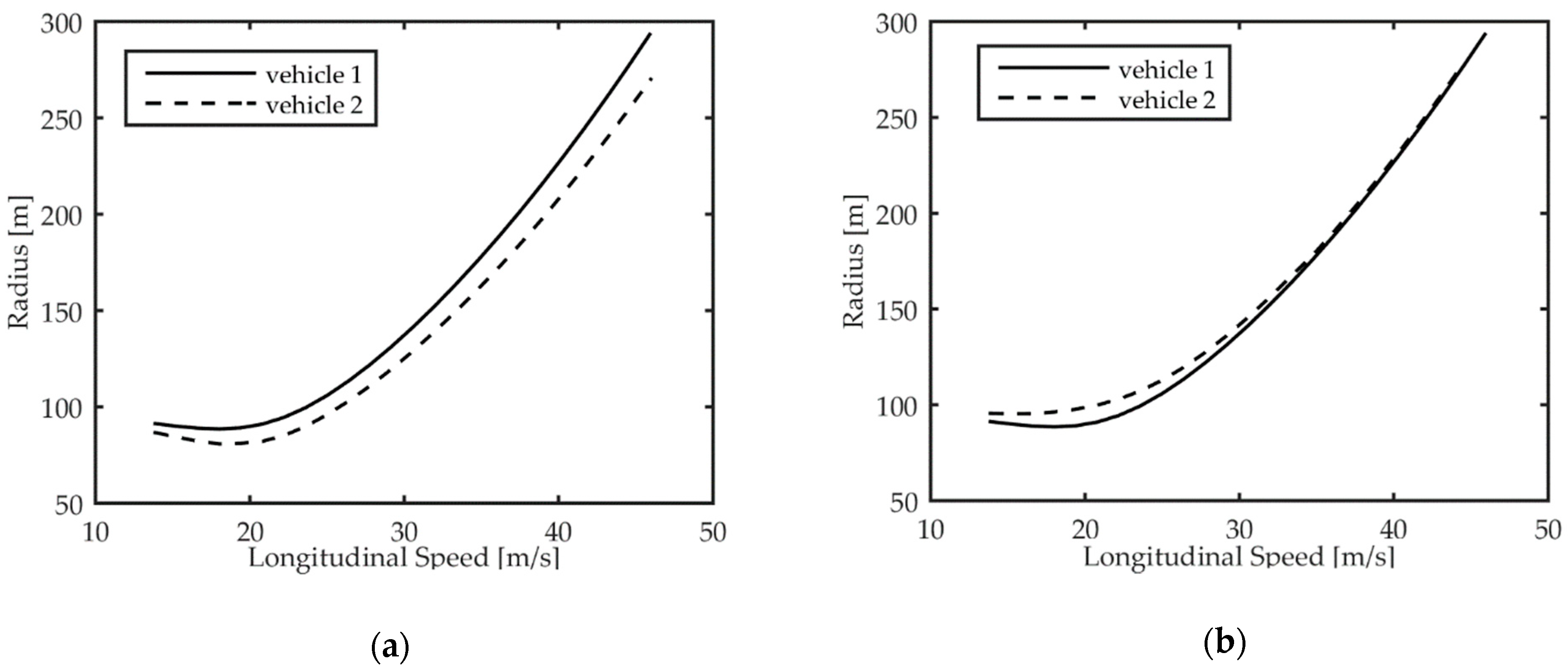
Figure 11 shows the turning radius as a function of the longitudinal speed, measured in steady-state conditions during the CS test conducted by driver 2, which further clarifies the differences in the lateral behaviour of two test vehicles.
As expected, for a given value of the longitudinal velocity controlled by driver 2 as indicated in
Section 3, due to the higher oversteering in driving mode 1, vehicle 2 travels along circular paths with a radius that is lower than the one exhibited by vehicle 1. Instead, when driving mode 2 is selected, the DYC forces vehicle 2 to travel along higher-radius circular trajectories as compared to vehicle 1.
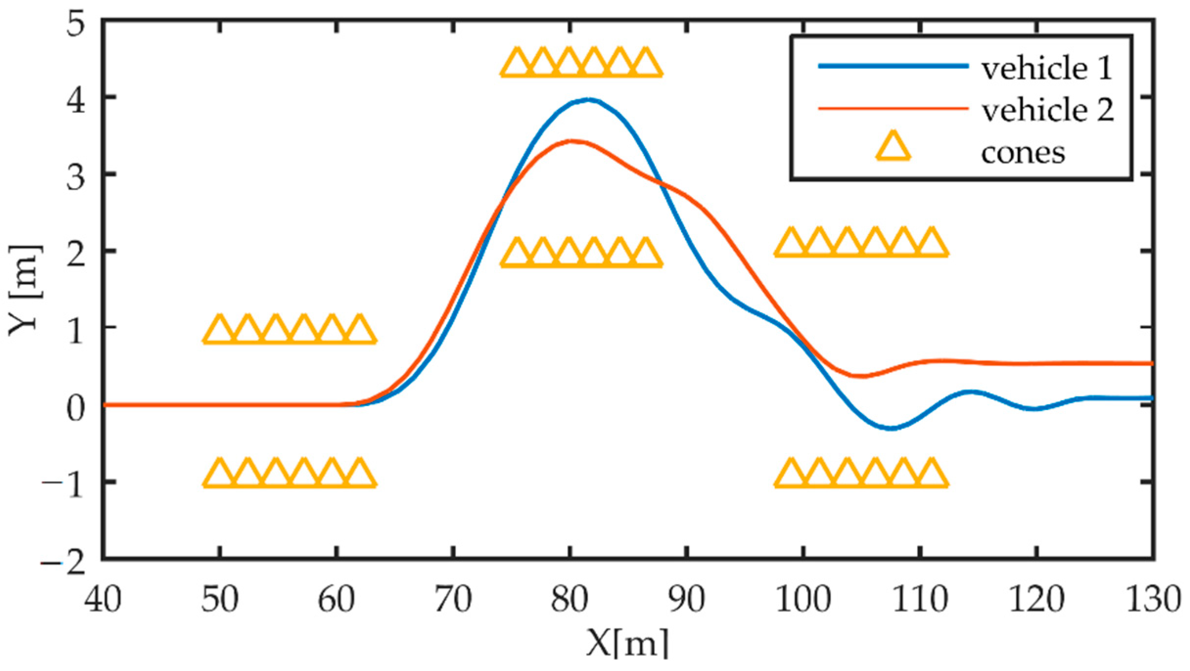
The effects of TV on the lateral dynamic response of the two vehicles are evaluated also using driver 3 to perform the SLC testing manoeuvre. In this test, driver 3 drives the vehicle until
Section 1 of the test track by achieving a longitudinal speed of 14 m/s. With this entry speed value, driver 3 on vehicle 1 fails to complete the manoeuvre. Instead, due to the effects of DYC on the lateral dynamics, which enhances the oversteering performances, vehicle 2 is able to complete the driving test faultlessly.
Figure 12 shows the paths followed by the centres of gravity (CGs) of vehicle 1 and vehicle 2, along with the desired path during the manoeuvre. Considering the track dimensions defined in
Table 2 and a vehicle width of 1.4673 m for
Section 3 and
Section 5 of the test track, the maximum allowed absolute values of the position error are 0.5 and 0.76 m, respectively. Vehicle 2, subject to DYC in driving mode 1, proves able to correctly complete the manoeuvre, with a maximum position error of about 0.12 m. This is due to the higher level of oversteer that makes vehicle 2 more responsive to the driver’s steering input, allowing it to travel on a path with a lower-curvature radius than vehicle 1 at the same speed.
5. Conclusions
This paper proposed a C++ simulation platform for multiple and concurrent vDiL simulations of road vehicles. In the proposed scheme, a software driver, replacing the human driver interaction, calculates all the possible control signals such as throttle, brake, and steering angle, based on the asked manoeuvre and relying on a set of nested PID controllers. The preliminary evaluations of the simulator showed great potential for achieving the concurrent simulation of several vehicles.
Several variants of a vehicle can be simulated with different characteristics such as geometry, mass properties, tyres, and transmission. The simulation environment relies on a modular and hierarchical architecture, which can more naturally be further expanded in several ways: additional modules could be dedicated to perform other dynamic tests; other modules could create an interface with more advanced virtual driving scenario software; yet other modules could expand the current functionality implementing more complex hardware interfaces such as a motion platform. In this latter scenario, our simulator could be instrumental for comparing human-in-the-loop (HiL) with vDiL during closed-loop manoeuvres, similar to those presented in this study or even more complex driving scenarios on virtual tracks. Future works are planned to add modular and scalable-detail sub-system models and more advanced control strategies, such as fuzzy or predictive control models.
The advantages of using the vDiL approach have been illustrated. The reported test results demonstrate the capabilities of the proposed simulator and its effectiveness in evaluating the dynamic performance of multiple passenger cars with low computational impact. The possibility of instantiating several vehicles, even different variants of a vehicle, joined to the possibility of different virtual drivers has been achieved using the OOP paradigm. The resulting software environment represents a flexible tool for simulating different driving scenarios, enabling several research activities in line with the recent automotive industry demands.


 ,
, 


