Design and Control System Setup of an E-Pattern Omniwheeled Cellular Conveyor


Faculty of Electrical Engineering, Universiti Teknikal Malaysia Melaka, Hang Tuah Jaya, Durian Tunggal, Melaka 76100, Malaysia
*
Author to whom correspondence should be addressed.
Machines 2021, 9(2), 43; https://0-doi-org.brum.beds.ac.uk/10.3390/machines9020043
Submission received: 30 December 2020
/
Revised: 31 January 2021
/
Accepted: 7 February 2021
/
Published: 20 February 2021
(This article belongs to the Section Automation and Control Systems)
Abstract
:The addition of omnidirectional capability and modularization to conveyor systems is an exciting and trending topic in current conveyor research. The implementation of omnidirectional modular conveyors is foreseen as mandatory in the future of conveyor technologies due to their flexibility and efficiency. In this paper, an E-pattern omniwheeled cellular conveyor (EOCC) is first introduced. Camera and image processing techniques are utilized to achieve a centralized system, which is more robust than conventional decentralized systems. In order for cartons to maneuver across the EOCC, a unique method for activation of the actuators is subsequently designed. Next, the nominal characteristic of the EOCC is analyzed based on the step responses, which then inspire the proposal of four simple controllers, namely the P–P–P–P controller, + P–P–P–P controller, P–P–PD–PD controller, and + P–P–PD–PD controller (P for proportional, D for derivative and for time-shifting), which are used to evaluate the tracking performance of the EOCC in diagonal-shaped, ∞-shaped (horizontal lemniscus), and 8-shaped (vertical lemniscus) trajectories. The results show that there is no clear winner among the controllers, with each having its own advantages and disadvantages. Nevertheless, such findings provide clearer insight into the EOCC, which is vital for future works. After all, the introduction of the EOCC system in this paper is also anticipated to elevate the benchmarks and competitiveness in the current field of modern conveyor technologies.

1. Introduction
Smart factories and automation are two major factors in the fourth industrial revolution (4IR). Many industries have started to adhere to the principles of the 4IR, where their production rates are expected to increase significantly. High production rates alone are insufficient; in other words, the capability of the conveyors to handle high volumes is a prerequisite. Moreover, with the boom in e-commerce in recent years, which has now been accelerated by the global coronavirus pandemic, logistics is becoming a crucial topic to be discussed in research.
In logistics and conveyor technologies, carton carriers can be categorized into two general categories—with and without mobility. Forklifts and hand pallet trucks are examples of mobile carriers used in logistics, whereas belt and roller conveyors are non-mobile carriers. A study [1] further categorizes these carton carriers based on their throughput performance. The results of the comparison are shown in Figure 1. Mobile carriers are agile, however, have low throughput, whereas non-mobile carriers have higher throughput, yet with non-existent mobility. In an effort to overcome these gaps, a mobile belt conveyor has been proposed. However, it is bulky and not deemed fit for congested environments. Moreover, belt and roller conveyors are limited to unidirectional transportation with cartons of a predefined size. Therefore, even though mobility can be added to reinforce existing belt conveyors, there is still plenty of room to improve the throughput performance. As a result, researchers have been proposing and studying modular or cellular conveyors over the past decade, and foresee such technologies as being essential in the field of logistics amid the fourth industrial revolution [2,3].
In order for a carton carrier to be classified as a cellular conveyor, a prerequisite characteristic is modularity. Modularity allows combinations of multiple carriers with no restrictions. Therefore, the layout of the overall conveyor system or transportation line can be modified using a “plug-and-work” approach without any hassle or major reworking. Faulty cells or modules can also be replaced easily [4]. In other words, modularity enables flexibility and adaptability. Since cellular conveyors are in the form of arrays, faulty cells or modules can be bypassed and temporarily supported by neighboring cells in cases of emergency, without stopping the entire transportation line for repairs. Additionally, cellular conveyors can be either unidirectional or omnidirectional. As seen in Figure 1, such modular characteristics make cellular conveyors desirable among other conventional logistic carriers. Therefore, cellular conveyors are deemed fit to be applied in real life across many industries.
Cellular conveyors are proven to be capable of working with conventional logistics carriers, but conveyor system layout optimization [5,6] and integrated software [7] are needed. The deployment of a cellular conveyor has had positive results in many real-life applications, such as robust sorting processes in courier companies [5], semiconductor applications for the transportation of wafer [8], and sorting processes in warehousing [9]. Regardless of the industry, as long as complex transportation and sorting are involved, cellular conveyors are capable of forming efficient automated sorting systems [5,10]. In fact, almost every large industry today requires complex transportation and sorting in back-end processes. Based on the illustration in Figure 2, an array of cellular conveyors is capable of creating multiple inbound and outbound channels, allowing cartons of different sizes to be moved, whereas for roller and belt conveyors, cartons can only be moved in to-and-fro directions and with limited or prescribed carton sizes. Overall, cellular conveyors are better at effectively utilizing the working area. In the upcoming sections, a literature review on how omnidirectional capability and modularity come into existence and how they affect current logistics and conveyor technologies will be presented.
1.1. Omnidirectionality and Modularity in Conveyor Technologies
As early as the 1920s and 1970s, the Omni wheel and Mecanum wheel were introduced, respectively, to realize omnidirectional capability [11,12]. Back then, the benefit of omnidirectional capability was significant, but its industrial application was only brought into limelight among the engineers and researchers by late 19th century. Omnidirectional capability has the potential to improve throughput in many real-life applications, including logistics. Oyobe et al. proposed a material flow system that is capable of conveying object omnidirectionally. Multiple z-directional operating actuators worked in a central–decentralized control manner. Subsequent upward movement by the actuators realized a conveying transportation. Proportional–derivative controller with disturbance observer was proposed to control point-to-point positioning of a carton or object. Even though the z-directional actuator may be impractical for logistics at such an early stage, it is certainly a groundwork to promote and realize omnidirectional capability among conveyors [13].
A study [1] proposed a cellular conveyor known as “Flexconveyor” back in 2009, which can be considered one of the earliest cellular conveyors based on extant literature. Flexconveyor is made up of rollers for longitudinal motion and diverters for latitudinal motion. The diverters are hidden under the rollers, and will be lifted up whenever needed. The rollers in each Flexconveyor cell are mechanically joined, and therefore they actuate synchronously. A similar synchronized mechanical structure is applied for the diverters. As a result, Flexconveyor is incapable of realizing the yaw or orientation control of the carton and is therefore categorized as unidirectional cellular conveyor. Each Flexconveyor cell is equipped with a photoresistor and RFID reader to detect and identify the carton, respectively. The Flexconveyor cell also has four communication interfaces at each side so that communication with neighboring cells can be established. When there is a need to change the layout of the whole conveyor system, each Flexconveyor cell can be moved and relocated easily, as caster wheels are installed to each cell. In terms of control system, a decentralized control method was proposed by the author, where each cell is operating on its own based on the instruction received from or passed down by neighboring cells. The modularity concept by Flexconveyor is certainly a breakthrough from traditional conveyor systems despite its inability to produce yaw control and demand for extra lifting actuation for the inverter.
Since then, many types of new conveyors based on the concepts of modularity and omnidirectional capability have been proposed. Furmans et al. propose KARIS, a cellular conveyor like the Flexconveyor. KARIS, an automated guided vehicle (AGV), is introduced; therefore, relocation process can be done automatically [3]. Next, a series of new omnidirectional cellular conveyors known as “small-scaled conveyor modules” (SCM) is proposed. These conveyor modules are either made up of servo driven swiveling roller, belt driven swiveling roller, axial piston, or rotating swash plate. In the belt driven swiveling roller conveyor module, each row of rollers is mechanically joined. However, in terms of the servo driven swiveling roller, axial piston, and rotating swash plate conveyor module, each module has only one actuator to be controlled. As a result, the belt driven swiveling roller conveyor module may be simpler in terms of mechanical structure and control system, yet is unable to perform yaw control like others [14,15,16,17]. Other than the small-scaled conveyor module that uses swiveling concept, omniwheel is widely recommended as well. Wang et al. uses the small size and big size of omniwheels to realize a conveyor platform with omnidirectional capability. The conveyor platform is nonmodular and each row of omniwheels is mechanically joined. Wafer lots are transported flexibly between two different production lines without wasting time on queuing up before lots [8]. A combination of omniwheel and driving gear that forms a treadmill belt is also proposed to realize an omnidirectional conveyor platform [18,19,20]. These above-mentioned efforts in conveyor technologies are promising in improving throughput and efficiency; however, they are nonmodular types of conveyors. Regardless, a study [20] foresees the importance of modularity. The study proposed the treadmill being segmented into modular as an effort for future work. Uriarte et al. proposed Celluveyor—a one-of-a-kind hexagonal-shaped cellular conveyor that is made up of three omniwheels that are similar in size [2].
For better overview and comparison, Figure 3 shows the physical appearance of the above-mentioned conveyors. Even though Flexconveyor and conveyors with big–mall omniwheels (BSO) are incapable of producing yaw control, they are more economical and efficient, as they have bigger diverter wheels and omniwheels, respectively, to transport cartons farther per rotation. Meanwhile, SCM and BSO have higher resolutions than others as their wheels are arranged closely together, hence easing the handling of smaller cartons. The SMC has only small wheels, and it is so compact that in most situations, it may be less economical, yet with a sophisticated control system. Overall, the BSO is economical with decent resolution, but it could not produce yaw control. Therefore, this paper proposed the modularization of a conveyor platform comprising big and small omniwheels—E-pattern omniwheeled cellular conveyor (EOCC). As a result, yaw control can still be achieved while maintaining the economical and resolution properties. The design, setup, and control system of the EOCC, the highlights of this paper, are to be discussed in the upcoming sections. Even though many types of omnidirectional modular conveyors have been introduced over the past decades, the introduction of EOCC by this study is expected to elevate the benchmark and competitiveness in the field of modern conveyor technologies.
1.2. Existing Control System
A cellular or modular conveyor system involves multiple cells working together cooperatively, whereas omnidirectionality indicates omnidirectional maneuvering transportation of an object or carton. Each of the conveyor cells consists of multiple actuators to be controlled constantly. Therefore, the control system for the omnidirectional cellular conveyor is expected to be complicated in most circumstances. The existing control system for the conveyor in the literature can be categorized into the decentralized control system and centralized control system. Generally, in the decentralized control system (DCS), each cell receives command and information from neighboring cells and then decides its corresponding action, whereas in the centralized control system (CCS), a centralized controller such as a computer exists to supervise and decide the action of each cell. CCS often has vision on the whole conveyor system, either through bird’s eye view camera or continuous feedback data from all cells, whereas for DCS, there is no centralized “brain” to decide the actions of all the cells. Instead, each cell is equipped with a microprocessor to perform actuation on its own, based on pre-programmed logic, current state, and the data received from neighboring cells.
Based on literature, DCS is more widely used than CCS. DCS is proposed for Flexconveyor, and each Flexconveyor cell is equipped with on-board computer, RFID, proximity sensors, and communication ports on each side [1]. Each cell is responsible for making decisions, controlling its actuator, and communicating with neighboring cells. As information passing from the first cell or module to its neighbors may take some time, Oyobe et al. proposed a central–decentralized control system, where a central computer will be sending out commands to several modules at the boundary at one time in order to improve the communication efficiency [13]. Next, DCS is also proposed for small-scaled conveyor module. The module is equipped with control board, light sensors, and communication interface [14,16,17]. Similar to other decentralized structures, the sensor provides feedback to its own module and neighboring modules. Therefore, the control algorithm for DCS is challenging, because the algorithm needs to perform appropriate action merely based on the feedbacked logic states without having a complete and precise view on the whole conveyor system [5,21,22]. The DCS also does not have vision on the exact location of the carton. Hence, grouping the cells or modules into a neighborhood is proposed to achieve continuous or non-jerking flow of the carton. This neighborhood size and pattern vary based on the size of the carton, thus allowing different sizes of carton to be transported on the conveyor platform [14,15,16]. The method of neighborhood in DCS was inspired by Cellular Automata [23,24]. Since the DCS does not have vision on the whole conveyor platform, the route for the carton to travel is dynamic based on the states of other conveyor cells or modules, which are updated from time to time [15,21].
In CCS, a centralized computer exists in order to command the actuation of each cell or module. A centralized sensor such as camera is in action to read the state of each cell. With some advanced image processing techniques, the CCS, then, has vision on the whole conveyor system, including the size and quantity of carton as well. Unlike DCS, the conveyor cell or module in CCS is usually equipped with only actuators and driver board. The communication between the central computer and all the cells can be established via hard wiring, or wirelessly through the concept of Internet of Things (IoT) system as promoted for cellular conveyor and warehousing [9]. Uriarte et al. proposed a centralized system for Celluveyor. In the study, a camera with depth sensing capability is used, where images and depth data are combined via several processing techniques such as contour detection, green theorem, and others to realize accurate detection of the carton [2].
Both the DCS and CCS have their respective pros and cons. In terms of hardware, the decentralized system is more complicated than the centralized one, because the former requires on-board computer and sensors on each cell. In contrast, the utilization of camera in CCS has the advantage of visualizing multiple conveyor cells or even whole conveyor systems precisely without requiring any on-board sensors. However, ensuring the sufficient surround ambient light intensity and unblocked camera view could be challenging for the CCS. As for DCS, transportation of the carton can still be realized without a complete vision on the whole conveyor system, yet methods such as neighborhood, dynamic routing, and others are necessary. In DCS, the physical dimension of the carton is just an estimation based on the feedback states by the conveyor cells, whereas in CCS, the size can be determined via camera vision and some image processing techniques.
Even though DCS is more common in the literature, Spindler et al. argued that CCS is more intuitive and considered as the state-of-the-art in the logistics industry [7]. Application of camera vision is handy and easily accessible today, and is much simpler and effective than placing on-board sensors on each conveyor module. Moreover, image processing techniques are becoming more and more robust, mainly due to the thriving of artificial intelligence throughout the last decade. Hence, this paper proposed E-pattern omniwheeled cellular conveyor (EOCC) based on the concept of centralized control system (CCS), which is to be presented in Section 2.
1.3. Existing Controller
A merely decentralized control system (DCS) or centralized control system (CCS) is insufficient for omnidirectional cellular conveyor to achieve precise transportation of the carton. Control theory is utilized to realize decent point-to-point and trajectory tracking performances. Based on literature, not many controllers are discussed and proposed for the omnidirectional cellular conveyor. Typically, a proportional–-integral–derivative (PID) controller is mostly proposed. PD controller with disturbance observer is proposed for a central-DCS omnidirectional conveyor platform with z-directional actuator, known as Magic Carpet. Meanwhile, variable structure controller is also proposed to control the displacement of each of the z-directional actuator, so that gradient surface can be formed for object to “flow” from one position to another [13]. Uriarte et al. implemented a PID controller for angle control and a velocity vector controller for positioning control in Celluveyor [2]. The Celluveyor has a CCS structure. Point-to-point experiments have been conducted to evaluate the performance of the proposed overall control system. Next, Pyo et al. proposed two PD controllers to control x-directional and y-directional speeds of an omnidirectional platform known as Fast-Omnidirectional Treadmill (F-ODT). The F-ODT is in the category of CCS. The reason why two controllers with different tuned parameters are needed is because the properties of x-directional actuator and y-directional actuator are different due to different gear ratio, physical properties, and others. In a study [19], sinusoidal path tracking experiment for speed control has been conducted. A PID controller with anti-windup scheme is proposed for a CCS to control the positioning of two objects simultaneously [20]. As a result, the proposed controller is able to realize tracking of a complex-shaped path.
Based on the review of literature, most of the proposed PID controllers come with additional schemes such as disturbance observer, anti-windup, and others in order to realize path tracking performance. Pendleton et al. suggested that the PID controller can be tuned intuitively without determining an accurate system model, but it has the limitation of delayed response towards error. This delay causes a restriction to a trajectory tracking experiment or application [25]. Normey-Rico et al. proposed a PID controller with additional robust tuning parameter in order to realize tracking of an arbitrary path. This additional element is deemed essential as well [26]. Similarly, in this study, time shifting element was introduced to the P–P–P–P controller and P–P–PD–PD controller for the EOCC in trajectory tracking performance.
2. Materials and Methods
This section comprehensively introduces the design and details of the proposed E-pattern omniwheeled cellular conveyor (EOCC), from physical structure to functioning control system. Trajectory tracking experiments were simulated to justify the validity of the designs in this paper.
2.1. Environment Setup
E-pattern omniwheeled cellular conveyor (EOCC) is a cellular conveyor with capability to transport the carton omnidirectionally. Each cell is made up of two types of omniwheels, in which one is bigger than the other in terms of diameter. Specifically, the diameter difference is in a ratio of around 1:3. These omniwheels are arranged in such a way that one big omniwheel is perpendicular to three small omniwheels side by side. Eventually, they form a pattern that looks like an “E”, which is made up of one vertical line and three horizontal lines. The physical appearance of one EOCC cell is as shown in Figure 4.
As mentioned in the last section, a combination of big and small omniwheels is more economical than using only small omniwheels. The “E”-shaped wheel arrangement in the EOCC allows yaw control on the carton in the midst of transportation. Figure 4 shows the computer-aided design of the EOCC cell designed by using SolidWorks software. To evaluate the functionality and performance of the EOCC, Virtual Robot Experimentation Platform (V-REP) software (known as CoppeliaSim now) is used to create a simulated environment. V-REP is an open-source platform used to simulate robotics and automation. Pitonakova et al. presents a thorough comparison between V-REP and another well-known simulation software known as Gazebo. Gazebo is said to be capable of simulating a larger environment and larger number of robots than V-REP [27]. Gazebo is also validated in terms of performance and modelling by using a simple differential robot, and the outcome is promising [28]. Gazebo has limitations in restructuring the meshes of the imported object, and has no interface with Python programming language, whereas V-REP is more flexible in meshing and has built-in Application Programming Interface (API) for Python programming language. Moreover, the modelling of omniwheel in V-REP is very intuitive due to the available abundant default models that come together with the software for user reference. Even though Pitonakova et al. suggested that V-REP is incapable of simulating a large environment, in this paper, a large environment—42 EOCC cells comprising 147 actuators (DC motors) in total—was successfully simulated. Methods on how to setup and optimize this simulation environment are presented in upcoming paragraphs and subsections.
An omniwheel is a type of wheel where its circumference is made up of rollers. The axis of each roller is perpendicular with the axis of rotation of the omniwheel. A conventional wheel can be modelled as a cylinder; thus, the contact region between the wheel and floor or object is a line of contact. In terms of the omniwheel, due to the presence of rollers, the contact region is a point of contact. This is also the reason why the omniwheel experiences slippage more easily than a conventional wheel [29,30,31]. Nevertheless, due to the point of contact, the omniwheel can then be modelled using a sphere in V-REP. Figure 5 shows two spheres that are combined to represent the mechanism of an omniwheel. One of the spheres represents the wheel, whereas the other represents the roller. Therefore, two axes of rotation can be observed in Figure 5. Both the joints or axes are perpendicular to each other. For the roller joint, it is characterized as frictionless, just like a free rotating roller in real life, whereas for the wheel joint, the joint is motor-enabled and therefore acts like a driving motor in real life. The wheel sphere model and roller sphere model appear to be physically overlapping and crashing with each other. In fact, only the roller sphere is configured as “respondable” in the V-REP simulation environment, suggesting that only the roller sphere is responsive towards external forces. Next, based on Figure 5, two of the big omniwheels are close to each other, and therefore their adjacent roller spheres will be slightly touching or collapsing on each other. To solve this issue, all the roller spheres that touch adjacent roller spheres are assigned into different “respondable mask” layers so that from V-REP’s point of view, they are not collapsing on each other. Once modelling of the big omniwheel is completed, a similar modelling idea is applied to the smaller omniwheel of the EOCC cell.
In the experimental setup of this study, the EOCC platform is shown in Figure 6. The platform was made up of 42 EOCC cells arranged in 6 × 7 array form. Each cell had physical dimensions of 0.250 m (L) × 0.217 m (W). Overall, the EOCC platform was measured at 1.50 m (L) × 1.52 m (W). In order to realize a centralized control system for the platform, a camera was installed at the top as feedback sensor to obtain a bird’s-eye view. The camera was set with perspective mode and resolution of 256 × 256 pixels. A Python script was written to communicate with the camera (sensor) and motor-enabled joints (actuator) via V-REP’s built-in Python API, thus achieving a closed-loop control system for the EOCC. Besides the provided handy API, Python programming language was chosen for this experiment because it was well supported with many frameworks, especially machine vision (OpenCV) and data science tools. Next, the maximum speeds for the big omniwheel and small omniwheel were limited at approximately 0.20 ms−1, which were around 20 and 60 RPM, respectively. As a large number of actuators were involved during the simulation, it was mandatory to run the simulation and programming script in synchronized mode. In other words, at each discrete timestep, the script would be waiting for the V-REP to complete its calculation first before executing the next command. The same goes for the situation where V-REP waited to be triggered by the script at each timestep, hence ensuring the simulation performed was valid and optimal. The time step set for all the experiments in this study was 20 ms.
2.2. Control System Design
In this subsection, the control system designed for the E-pattern omniwheeled cellular conveyor (EOCC) is explained in detailed. The control system designed was a centralized type, because each EOCC cell was not equipped with an on-board sensor and microprocessor. Instead, a camera was used as a centralized sensor to determine the state of each EOCC cell, and a Python script, which acted as a centralized processor, was executed to perform, read, and control. Generally, a typical control system block diagram (as shown in Figure 7) should consist of a “feedback” block, a “controller” block, and a “process” block. Therefore, in this subsection, each of these blocks in the EOCC control system is introduced one by one by how it is designed. Additionally, at the end of this subsection, the EOCC platform was tested in open-loop and closed-loop preliminarily in order to visualize and understand its nominal characteristic.
2.2.1. Design of “Feedback” Block
The breakthrough of neural networks in image processing over the past decades has enabled machine vision to become more powerful than before. Industrial cameras with improved resolution, frame rate, low-light imaging, and others are easily accessible today. These are the reasons why a camera was selected as the sensor for the EOCC in this study. In addition, as mentioned in the literature section earlier, the centralized control system is predicted to be state-of-the-art among future cellular conveyor systems, partly due to the current advancement of machine vision technologies.
In the EOCC simulation environment, the bird’s-eye view camera was to perform two main tasks: to determine the state of each omniwheel and absolute position of the carton. Both tasks had to be conducted in a continuous manner. Figure 8a shows the raw image captured by the camera in the simulated environment. As the computer used to perform the simulation in this study had limited processing power, the colored image captured by the camera had resolution of only 256 × 256 pixels. Regardless, the omniwheels in the image could still be clearly identified from a human’s perspective, where their positions could be determined. Next, in this paper, the positions of the omniwheels in the raw image were determined manually. A red rectangle was drawn manually on the raw image as shown in Figure 8b, representing the boundary of the omniwheel. In real-life application, a bright colored boundary can be painted or marked directly on the physical body of the EOCC cell, so that through image processing, the centralized computer can directly determine the position of each omniwheel without requiring any manual drawing. Alternatively, feature matching or a neural-network based classifier can be used to easily locate these omniwheels in real life.
Once boundaries were done as shown in Figure 8b, the image was then processed to obtain the center coordinate of each red rectangle, representing the “address” of the omniwheel. The general steps of the image processing were as follows:
- Threshold values were set so that only red pixels remained in the image. Non-red pixels were masked as black as shown in Figure 8c.
- The image was then converted to grayscale and followed by thresholding the image. Each pixel was now in binary form, either white or black, easing the next processing stage.
- All closed contours were extracted from the image by using the contours-finding function in OpenCV library [32].
- Each contour with rectangular shape was accepted and then classified into either the “big omniwheel” or “small omniwheel” category based on its bounding area.
- Information of each omniwheel such as omniwheel category, contour center coordinate, index, and naming in V-REP software were compiled and stored in a database.
With this database ready and available, the central processor (a Python script as main program in this case) was, then, able to control all the omniwheels (actuators) in the simulated environment based on the image from camera. The final image for this processing stage is as shown in Figure 8c, and it works as an important reference image for the control system of the EOCC platform together with the database, which will be explained in the upcoming paragraphs.
The common carton in real life is usually brown in color. However, it can also be customized and standardized into any preferred color. Therefore, detecting the presence of the carton is simple, but determining the states (absolute position and orientation) of the carton is more challenging. Figure 9a shows an image of the carton on the EOCC platform captured by a camera. Through simple image processing, non-carton (non-brown) pixels were masked as black as shown in Figure 9b. Next, the steps of obtaining the carton’s absolute position were as follows:
- Converting the image to grayscale, as shown in Figure 9b, followed by image thresholding to binarize the pixel.
- Obtaining the contour that represented the carton by using the contour-finding function.
- Based on the contour, the number of vertices the contour had was approximated by using the Douglas–Peucker polynomial curves estimation method [33]. The carton should have four vertices.
- From the coordinates of these vertices, the length and width of the carton were then calculated. By taking their midpoints, the center coordinate (position) of the carton could, then, be determined.
Next, in order to determine the absolute orientation of the carton, two points were needed to form an inclined line. The center coordinate point of the carton and reference point at time were the points used. Based on Figure 9c, a blue vertical line appeared within the carton. The blue line connected the center of the carton and the reference point. The reference point was also the midpoint of the edge. Equation (1) shows the formula of calculating the absolute orientation of the carton, at time ,
where and . The absolute orientation of the carton, , ranges from 0° up to 180° and from −1° up to −179°. Figure 9c shows the final processed image, with “(128, 128, 0)” indicating the center coordinate and orientation of the carton. The center coordinate “(128, 128)” is in the unit of “pixel (px)”. The origin (0 px, 0 px) of the image was located at the top-left corner of the image. This proposed method successfully realized a robust positioning and orientation feedback for one carton. For cases with multiple cartons in the future, identification and tracking of the cartons can be easily be realized by using the Hungarian algorithm [2].
To be precise, the “feedback” block did not only provide the carton’s position and orientation to the “controller” block. In fact, it also offered actuator activation information. As mentioned in the introduction section of this paper, the cellular conveyor involves a large number of actuators working together cooperatively. Therefore, supplementary methods such as Von Neumann neighborhood, Moore neighborhood, and others have been proposed in the literature. In this paper, the cross-then-activate method was proposed instead. The executional flow of the method was as follows:
- The pixels of the image in Figure 9b were first binarized and then inverted to create a mask. The mask was then combined with Figure 8c via bitwise “AND” operation. As a result, all the red rectangles’ edges that lay within the carton were erased, leaving some red rectangles with incomplete perimeters.
- Red rectangles with incomplete or broken perimeters were not considered as a contour, and hence were eliminated, whereas the addresses of red rectangles with complete perimeters were recorded and passed on to the “controller” block.
- The “controller” block compared these addresses with the reference addresses stored in the database to know which actuators to be activated and deactivated.
To enable a better visualization, the rectangles that were crossed by the carton were colored green. For a better understanding, Figure 10 shows a series of processed images at different time step during one of the experiments conducted in this paper.
Compared with the neighborhood method mentioned in the literature, the proposed cross-then-activate method is more efficient and effective. It reduces the amount of time and number of actuators idling and waiting for the arrival of the carton. In fact, as soon as the carton crosses the border of the rectangle, which is also right before the carton contacts the contact point of the omniwheel, the actuator is activated. In the experimental result section of this paper, the proposed cross-then-activate method is validated, and it displays a promising result.
2.2.2. Understanding “Process” Block
As mentioned, the proposed E-pattern omniwheeled cellular conveyor (EOCC) cell was made up of small omniwheels and big omniwheels, controlling x-directional (lateral) and y-directional (longitudinal) motions, respectively. Therefore, both the motions were expected to exhibit different properties. It is important to understand and analyze the nominal characteristic of the EOCC, especially in terms of system nonlinearity and uncertainty prior to designing its controller and control system. In this subsection, open-loop and closed-loop step responses of the EOCC were presented to visualize the system characteristics in general. The mass of the carton was set to 10 kg throughout all experiments in this paper.
Two starting points viz. (128 px, 128 px) and (102 px, 173 px) were used to obtain the step response of the EOCC, as shown in Figure 11a,b, respectively. By comparing these two starting positions, the number of actuators (big and small omniwheels) involved to kickstart a step input actuation were different. Figure 11c,d show the step responses of the small omniwheels at different RPMs and at starting positions of (128 px, 128 px) and (102 px, 173 px), respectively. Symbol delta (Δ) denotes the difference between instantaneous position and respective starting position, which is also the change of value during the response. Both results at different starting positions depicted similar actuation properties, even though there were some dissimilarities and jittering, probably due to vision camera feedback noise and distortion. At time equals to 1000 ms, the “gaps” (differences) between consecutive ΔX-Positions were similar. Additionally, starting from 100 ms, the actuation curves were almost linear with respect to time. Therefore, it can be concluded that the small omniwheels of the EOCC platform do not display much nonlinearity during actuation, except that there is a time delay of approximately 100 to 200 ms at the beginning of the actuation. It is important to mention this time delay visualized from the nominal characteristic to ease designing the system controller later.
Next, Figure 11e,f show the step responses of big omniwheels at starting positions (128 px, 128 px) and (102 px, 173 px), respectively. Significantly, dissimilarity between them can be clearly identified, especially at high RPMs. The “gaps” between consecutive ΔY-Positions at 1000 ms were inconsistent, in other words, varying based on different input RPM values. Moreover, it can be observed that the curves at higher RPMs were nonlinear with respect to time. This nonlinearity was different at starting positions of (128 px, 128 px) and (102 px, 173 px). Since the characteristic of the Y-Positional (big omniwheels) actuation is based on location, this justifies the presence of uncertainty in the control system of the EOCC system. Conclusively, the actuation by the big omniwheels portrays significant nonlinearity and uncertainty, and also with time delay of approximately 100 ms.
After the open-loop lateral (X-axis) and longitudinal (Y-axis) motions analyses, the EOCC was proceeded with closed-loop analysis in term of Z-axis motion, which was the orientation control of the carton. The presence of the previously mentioned time delay, nonlinearity, and uncertainty properties in the characteristic of the EOCC were expected to affect the orientation control. In addition, Z-axis motion involved big and small omniwheels to actuate in a simultaneous, cooperative, and controlled manner. Therefore, hypothetically, the orientation control will be more challenging than the linear motion control.
Two simple proportional–derivative (PD) controllers were used to realize simple orientation control. The first PD controller, with proportional gain and derivative gain of 1.0 and 100, respectively, was used to control the speed of small omniwheels. The second PD controller, with proportional gain and derivative gain of 0.5 and 100, respectively, was used to control the big omniwheels. Figure 12 displays the closed-loop step response of the EOCC when a step reference value of 180° was inputted into its control system. The starting position of the response was (128 px, 128 px), as shown in Figure 11a.
Based on Figure 12, it can be observed that the PD–PD controller produced a smooth motion control to reach 180° (0° angle error) with minor overshoot. At the same time, slight deviation in X-Position and Y-Position could be observed during the orientation control. It is essential to note that for results in Figure 12, no controller was implemented for X-Position and Y-Position controls, only a PD–PD controller was implemented for angle (orientation) control. Next, this setup was validated with more different starting locations such as (128 px, 88 px), (128 px, 168 px), (82 px, 87 px), and (107 px, 173 px), which can be referred from Appendix A. These starting locations were unique and unlike each other. In other words, at these starting locations, the number of small and big omniwheels involved at that instance were different. Therefore, it is important to study and then understand the EOCC system thoroughly prior to designing the controller and control system. The step responses at these locations with step input reference value of 180° are shown in Figure 13.
Even though the PD–PD controller with the exact tuning parameters performed well at starting location of (128 px, 128 px), as shown in Figure 12, at different starting locations, dissimilar closed-loop performance was produced, as shown in Figure 13. Larger overshoot in angle and deviations in X-Position and Y-Position were significantly observed. Conclusively, the EOCC displays different nominal characteristics at different locations, which further justifies the presence of uncertainty in the system.
Based on the analysis done in this subsection, a clear understanding of the characteristics of the EOCC system can now be drawn. Based on Figure 11, the presence of nonlinearity and uncertainty are significant at high RPMs; therefore, operating the EOCC at lower RPM may be more favorable. Additionally, based on Figure 12 and Figure 13, a step reference angle input produces inconsistent performance at different starting locations. It can be observed that at the beginning of these step responses, the effect was less significant and was yet to escalate. Therefore, based on these findings, trajectory input is deemed more suitable than step input and is then proposed to control the EOCC system. Complete details on the design of the controller are presented in the upcoming subsection.
2.2.3. Design of “Controller” Block
As the proposed E-pattern omniwheeled cellular conveyor (EOCC) in this study is relatively new and novel compared to the existing cellular conveyor, a simple controller was preferred to first enable the conveyor in achieving basic transportation of the carton. Regardless, precision is still essential. As the proportional–integral–derivative (PID) controller is the most common controller for industrial application currently, in this paper, a similar de facto is followed. The structure of the controller and overall control system are depicted in Figure 14.
From Figure 14, notations and denote reference input and actual output of the control system at time , respectively. As mentioned in the last subsection, trajectory input is more suitable than point-to-point (step) input for the EOCC; the reference input is therefore a time-varying variable. The trajectory or path for the carton to track is pre-generated prior to the start of the transportation, and this is common among all existing centralized conveyor system in the literature. The generation of for different types of path will be discussed in the upcoming section. Next, by tuning the parameter in the time shifting controller, reference input can be time-shifted, creating lead or lag. The purpose of time-shifting is to overcome the actuation delay mentioned in the last subsection. The time-shifting parameter acts as an extra degree of freedom to enhance the common P and PD controllers. When is set to 0, is actually equal to . Notation , which represents error, carries the meaning on how far or how much the actual output is deviating from desired (reference) value. In equation-wise explanation, is the difference between and in terms of X-axis, Y-axis, and Z-axis. Therefore, they are actually in the form of an array or list.
Based on Figure 14, the P–P–PD–PD controller is actually a parallel combination of two P and two PD controllers that are controlling the RPMs of big omniwheels and small omniwheels of the EOCC. Notation denotes proportional gain, whereby its superscripts “” and “” represent X-axis positioning control and by using small omniwheels, respectively. Superscripts “ ” and “” are then understandably representing Y-axis positioning control by using big omniwheels. Based on Figure 14, the first P controller is used to control the small omniwheels in X-axis positioning, whereas the second P controller is used to control the big omniwheels in Y-axis positioning. Next, notation denotes derivative gain of a PD controller. Superscript “” represents Z-axis control, which is also the orientation control of the carton. Therefore, one of the PD controllers was controlling the small omniwheels, and the other PD controller was controlling the big omniwheels. The “rotation direction decider” block contains a simple algorithm that decides the direction of rotation based on the feedbacked information. Generally, by taking the carton’s center coordinate as reference point, the direction of rotation of the omniwheel can then be determined based on which quadrant the wheel’s center coordinate (address) is located at that particular time instance.
The PD controllers in the block diagram were in discrete-time domain viz. z-domain, and can be written in an equation form as:
where is the sampling time of the experiment, which is 20 ms as mentioned earlier. The output of the controller, is in the unit of RPM. As from the perspective of programming, codes are executed line by line; therefore, the discrete-time PD controller is needed to be transformed to digital PD controller. Firstly, Equation (2) is rearranged into a transfer function form, as shown as Equation (3). Then, by applying inverse z-transform, Equation (4) is obtained.
From Equation (4), notation denotes th error. In other words, represents error at a particular instance, whereas means error that is one step earlier of that instance. Now, Equation (4) is intuitive from the perspective of line programming. The derivative term of the PD controller is also clearly showing that the rate of change of error affects the controller output . Finally, Equation (4) is written into timestep domain, as follows:
Based on the block diagram in Figure 14, once the controller outputs were computed, these outputs were passed through an RPM limiter block so that the big omniwheel and small omniwheel of the EOCC were limited to operate at approximately 0.20 ms−1, which were around 20 and 60 RPM, respectively. The reason for defining this limitation is to ensure both the big omniwheels and small omniwheels have almost equivalent speed, and also to reduce the significance of wheel slippage at speed beyond 0.20 ms−1. Finally, the speeds for respective omniwheels will be summed up to create a resultant speed that will convey the carton on the EOCC platform.
Next, in order to validate the control system, the following controllers:
- P–P–P–P controller,
- + P–P–P–P controller,
- P–P–PD–PD controller, and
- + P–P–PD–PD controller
were used to perform evaluation on the trajectory tracking experiments. As the EOCC is relatively new and first proposed by this paper, starting with these simple controllers is preferred. A more advanced controller, control system, and tuning method will be discussed and presented in future works.
The value of was determined based on the time delay, as shown in Figure 11, which was around 100 ms. The final parametric values of the controllers are as shown in Table 1. During the trial-and-error and fine-tuning processes, a diagonal-shaped trajectory was used. For the tuning of the P–P–P–P controller, and were first set to 0. Then, both and increased by 1.0 in every test, until the X-axis and Y-axis tracking results started to show slight oscillation. The values of and were then decreased with step size of 0.1 until the oscillation in respective axes became insignificant. Next, it was proceeded with the tuning of and , which was similar with the tuning process of . and . Regardless, higher values of and could reduce Z-axis tracking error, but would cause the X-axis and Y-axis tracking results to overshoot. This occurred when fine-tuning with step size of 0.1 was carried out to leverage the compromise between these parameters. For the tuning of + P–P–P–P controller, similar steps were employed but with set to 100 at constant. Then, for the tuning of and , the derivative parameters increased with step size of 5 in each test until the best tracking performances were obtained.
The performances of these controllers in tracking various trajectories are later presented in the Section 3 of this paper, while for the upcoming subsection, the design and expression of the trajectories are first discussed. These selected trajectories have respective different shapes and complexity, which are vital in accurately validating the proposed control system and providing reliable scientific evaluation.
2.3. Design of Experiment
This subsection discusses how the experiment was designed to accurately evaluate the E-pattern omniwheeled cellular conveyor (EOCC) and its control system. The types of trajectory involved and the performance indexes employed to measure the trajectory tracking performances are presented.
2.3.1. Design of Trajectory
Three types of trajectories or paths were involved, namely diagonal-shaped trajectory, ∞-shaped trajectory, and 8-shaped trajectory. During each of these trajectory tracking experiments, the controller was required to gradually rotate the carton in a linear function of time. By the end of the trajectory, 360° of rotation was completed. Generation of the trajectory was a function of time by using a linear mapping formula as follows:
where denotes reference value or input to the control system. As mentioned in the last section, is actually equal to . In Equation (6), notations and denote input and output of the mapping formula, respectively. Taking the diagonal-shaped trajectory as example, the carton is desired to maneuver from position (75 px, 180 px) to (181 px, 74 px) within 6 s, as shown in Figure 15.
At starting position (75 px, 180 px) where ms, the desired or reference orientation was 0°, whereas at final position (180 px, 74, px) where ms, was 359°. Understandably, at the mid-point of the diagonal-shaped trajectory, the was approximately 180°. With all these conditions defined, can now be computed as follows:
Next, a similar method was applied for the generation of ∞-shaped and 8-shaped trajectories. As both the trajectories were longer in distance, the tracking duration set for them was 10 s instead of 6 s. The details of these trajectories are as stated in Figure 16. For the formulae of ∞-shaped trajectory and 8-shaped trajectory, the computation will be more complex, as unlike the diagonal, the relationship between and is now nonlinear. Regardless, the formula of ∞-shaped trajectory is as follows:
For the 8-shaped trajectory, its formula is just an inverse of the ∞-shaped trajectory, as follows:
A video that demonstrated the tracking of 8-shaped trajectory by the EOCC can be found at the ‘Supplementary Materials” of this paper. Generally, the diagonal-shaped trajectory is obviously much simpler, as it is only a straight path with minor challenge of 45° of maneuvering. For the ∞-shaped and 8-shaped trajectories, they comprehensively evaluate the capability of the control system in handling curved path. At the same time, the precision of the control system can be evaluated as well. Moreover, the ∞-shaped trajectory is relying more on small omniwheels of the EOCC, whereas the 8-shaped trajectory is on the big omniwheels. Therefore, both the trajectories serve respective important purposes. In upcoming subsection, performance indexes are introduced in order to analyze the performance from various perspectives.
2.3.2. Performance Indexes
The role of the performance index is to provide clear insight into the raw experimental data obtained. In this paper, integral of absolute error (IAE) and integral of square error (ISE) were employed to analyze the trajectory tracking performance of each controller.
IAE is basically a summation of all errors from each timestep of a complete trajectory tracking process. Due to the absolute properties, the negative sign of the error was disregarded. The formula of the IAE is as shown in Equation (15). IAE provides an overview to a trajectory tracking performance by showing how much tracking error in total by the end of the tracking experiment. Since the formula shown in Equation (15) is in continuous time domain, conversion to discrete form is needed. The result of the conversion is shown in Equation (16).
Next, the formula of integral of square error (ISE) is shown in Equation (17). The ISE works like a “scoreboard” as well due to integral term. However, with the square properties, the value of the error is subjected to exponential effect. Therefore, the ISE is sensitive towards large trajectory tracking error. Since high error is penalized, a more comprehensive analysis can be attained. The formula of the ISE is converted to discrete form as shown in Equation (18).
With the experiments and analysis methods designed and ready, the trajectory tracking experiments were then initiated. The outcome and results are presented and discussed in the next section.
3. Results
As mentioned in the previous section, experiments were conducted in a simulated environment of Virtual Robot Experimentation Platform (V-REP) software in order to validate the concept of the proposed E-pattern omniwheeled cellular conveyor (EOCC) and also the control system designed for it to function. Four types of controllers viz. P–P–P–P controller, + P–P–P–P controller, P–P–PD–PD controller, and + P–P–PD–PD controller were put to the test in the tracking of three types of trajectory viz. diagonal-shaped trajectory, ∞-shaped trajectory, and 8-shaped trajectory.
The upcoming experimental data collected were analyzed using integral of absolute error (IAE) and integral of square error (ISE). As mentioned previously, IAE sums up all the error of each of the timesteps, whereas ISE penalizes large error. It is noteworthy that the largest IAE value does not necessary produce the largest ISE value and vice versa. In addition, the IAE and ISE can hardly be estimated merely by observing the graphs. In other words, a decent looking trajectory tracking performance on the graph may have high IAE or ISE values and vice versa. Regardless, the use of performance indexes viz. IAE and ISE is still a more primary way of analyzing the result than observation, which can be considered secondary.
3.1. Diagonal-Shaped Trajectory Tracking
In this diagonal-shaped trajectory tracking experiment, the EOCC was required to maneuver the carton from position (75 px, 180 px) to position (181 px, 74 px). At the same time, the EOCC was required to rotate the carton in a gradual manner, and by the time it reached a final position, 360° of the rotation was completed. The simulated experimental results of this diagonal-shaped trajectory tracking using the earlier mentioned four controllers are as shown in Figure 17 and Figure 18. The results are also tabulated as shown in Table 2.
Figure 17 shows the trajectory tracking process by each of the controllers in a two-dimensional perspective. By comparing the results side-by-side, overshoot or oscillation occurred at the very beginning of the trajectory tracking by each controller. Among them, the P–P–P–P controller had the most significant oscillation, whereas the remaining had overshoot. To further analyze and compare their performances, the tracking data were broken down into axis form, which is as shown in Figure 18. Based on Figure 18 and in terms of X-Position Error axis, all four controllers had shown almost similar results, but if observed closely, + P–P–PD–PD controller had the least tracking error overall. Therefore, in the X-Position Error column of Table 1, + P–P–PD–PD controller scored the lowest IAE and ISE values viz. 292 and 364, respectively.
In terms of Y-Position Error axis, it can be observed that controlling Y-Position was more difficult than controlling X-Position. This circumstance is expected because of the nonlinearity of the EOCC, as mentioned in the Section 2 of this paper. In the same section as well, the EOCC also demonstrated system uncertainty during angle control. Based on Table 2, the + P–P–P–P controller had the best control in Y-Position, with IAE and ISE values of 145 and 187, respectively. After closely analyzing the results in Figure 18 and Table 2, one important finding can be discovered—by introducing the element to the P–P–P–P controller (forming a + P–P–P–P controller), it significantly improves performance in the Y-Position. However, if the derivative term is introduced to the P–P–P–P controller (forming a P–P–PD–PD controller), the Y-Position performance is slightly deteriorated.
Based on Figure 18 and in terms of angle error axis, it can be observed that for controllers that had the derivative term viz. P–P–PD–PD controller and + P–P–PD–PD controller, their angle controls were better than the other controllers that had no derivative term. Significant oscillation and high error were observed in the angle error axis of the P–P–P–P controller and + P–P–P–P controller. However, and surprisingly, in the “Angle” column of Table 2, the IAE and ISE values of the P–P–P–P controller were lower than the + P–P–PD–PD controller, even though significant oscillation was observed in angle error plot of the P–P–P–P controller but not in the + P–P–PD–PD controller. This situation may seem contradictory, but if the angle error plot of the + P–P–PD–PD controller was observed carefully, the tracking was above the reference line for a longer duration of the time. Therefore, this contributed to higher IAE and ISE values. Regardless, the derivative term did improve the angle error tracking performance, because the lowest IAE and ISE values were scored by the P–P–PD–PD controller.
3.2. ∞-Shaped Trajectory Tracking
Next, the controllers were proceeded to the next evaluation using the ∞-shaped trajectory. The tracking performances are shown in Figure 19 and Figure 20. Meanwhile, IAE and ISE values of these performances are as tabulated in Table 3. Based on Figure 19, significant oscillation and large tracking error were observed in the performances by the P–P–P–P controller and P–P–PD–PD controller. However, both the + P–P–P–P controller and + P–P–PD–PD displayed almost similar tracking performance in terms of X-Position and Y-Position. Intuitively, it can be preliminarily deduced that the presence of improves the positional tracking performance, which is also quite similar with the case of diagonal-shaped trajectory tracking.
Based on Figure 20, in terms of X-Position, all controllers displayed tracking performance. To be more precise, the + P–P–PD–PD controller and + P–P–P–P controller achieved the lowest IAE and ISE, respectively. Controllers that had no element showed higher IAE and ISE values in terms of X-Position. Next, a similar phenomenon occurred in Y-Position control as well, where the + P–P–P–P controller and + P–P–PD–PD controllers, which comprised the time shifting controller element , again achieved better Y-Position tracking performance than the P–P–P–P controller and P–P–PD–PD controller. Based on Table 3, + P–P–P–P controller achieved the lowest IAE and ISE values viz. 100 and 102, respectively. At the same time, the + P–P–PD–PD controller was slightly trailing behind the + P–P–P–P controller, whereas the remaining P–P–P–P controller and P–P–PD–PD controller were nowhere up to such decent performance.
Next, in terms of angle error control, the P–P–P–P controller suffered from slight oscillation. Based on Table 3, controllers that had derivative gain achieved lower IAE and ISE, with the P–P–PD–PD controller scoring the lowest IAE and ISE values of 727 and 1701, respectively. Even though the + P–P–P–P controller achieved impressive Y-Position tracking performance, as mentioned in the last paragraph, the controller showed almost the worst performance in angle control based on Table 3. Conclusively, the presence of the time shifting controller element significantly improves X-Position and Y-Position controls, and does affect angle control much, which is aligned with the finding in the aforementioned diagonal-shape trajectory tracking. Additionally, the derivative gain does improve angle control and also does not affect the positional tracking performance much. In this ∞-shaped trajectory tracking experiment, it is obvious that, overall, the + P–P–PD–PD controller outperforms others, even though the controller does not score highly on the lowest IAE and ISE values.
3.3. 8-Shaped Trajectory Tracking
In this subsection, the 8-shaped trajectory was used to evaluate the performances of the controllers. As mentioned earlier, the 8-shaped trajectory stresses the performance of the EOCC big omniwheels in Y-Position control more, whereas the ∞-shaped trajectory is vice-versa. Figure 21 and Figure 22 show the tracking results of the controllers on a Cartesian plane and in axes form, respectively. The IAE and ISE results are tabulated in Table 4.
Based on the plots in Figure 21, the + P–P–P–P controller was struggling to control the carton at the upper part of the 8-shaped trajectory. Significant tracking error was also observed in the tracking performance by the P–P–P–P controller and P–P–PD–PD controller. The + P–P–PD–PD controller achieved the best tracking result among all.
Based on the X-Position Error plot in Figure 22, all controllers displayed almost similar results. This observation is further supported by the IAE and ISE values in the X-Position column of Table 4, where their values were slightly different to each other. The controller that had the best X-Position tracking performance was the + P–P–PD–PD controller, with IAE value and ISE value of 420 and 536, respectively.
In terms of Y-Position control, the + P–P–PD–PD controller excelled all other controllers. In the previous result of diagonal-shaped and ∞-shaped trajectories tracking, it was found that the time shifting controller element helped to improve the positional tracking performance. However, this 8-shaped trajectory tracking case, with the addition of to the P–P–P–P controller (forming a + P–P–P–P controller) instead deteriorated the Y-Position tracking performance. This finding contradicted the findings in the previous trajectory tracking result. Regardless, the + P–P–P–P controller had poorer angle control performance than the P–P–P–P controller, which is similar to the previous findings.
Next, based on Figure 22 and Table 4, adding the derivative term to the P–P–P–P controller (forming a P–P–PD–PD controller) slightly improved the angle control and slightly degraded the positional control as well. In this 8-shaped trajectory tracking result, the + P–P–PD–PD controller showed the dominant performance among all, with the lowest IAE and ISE values in both the X-Position control and Y-Position control as shown in Table 4. Overall, the finding that can be drawn from the analysis in this 8-shaped trajectory tracking result is that the introduction of the element into the controller improves the positional control, which is similar to other trajectory tracking results. However, in terms of angle control, the derivative term only achieves a slight improvement, which is different from the previous trajectory tracking result.
4. Discussion and Conclusions
Based on the findings presented and discussed in the last section, it is found that the introduction of element improves positioning performance, but at the same time, it negatively affects angle control performance. In contrast, the introduction of derivative gain causes the other way around. Nevertheless, in the tracking result of 8-shaped trajectory tracking, such statements are partially correct, as the element has to work together with derivative gain in order to produce the best tracking performance; with only one of them, it does not produce the improved result, instead it may be worsened in terms of tracking error. As the 8-shaped trajectory tracking is highly dependent upon the big omniwheels, which exhibit nonlinearity and uncertainty properties as discussed in Section 2, it is more difficult to control these actuators. Conclusively, the overall findings show that a compromise to leverage the challenges is needed in order to obtain optimal tracking performance in all trajectories.
In summary, Section 1 of this paper serves as an introduction to conveyor technologies. The section begins with a problem statement discussion and how existing conveyor systems counteract the problem. By the end of the discussion, the scope is funneled into technologies such as omnidirectional and modular properties in existing conveyor systems. Furthermore, literature is presented and analyzed to determine the research gap, leading toward the motivation and desired contribution of this paper, which also includes the proposal of E-pattern omniwheeled cellular conveyor (EOCC) system. In the Section 2 of this paper, the design and setup of the EOCC are first presented and discussed. Then, the nominal characteristics of the EOCC control system are covered, analyzed, and presented. This finding is vital, as it provides a better understanding of the control system, leading to the idea of introducing a time shifting element and derivative gain to enhance a simple control system or controller. The idea is then comprehensively evaluated and discussed in Section 3 of this paper. Since the EOCC is relatively new and first introduced by this paper, the proposed control system and controller are intended to be simple and intuitive, yet match industrial de facto.
In the next milestone of this EOCC, the camera should be calibrated to overcome distortion so that nonlinearity of the sensing system can be suppressed. Most importantly, more cartons should be added and controlled simultaneously by the EOCC in upcoming works, and these cartons should have different mass and center of mass as well. This aim is vitally important, as it brings the EOCC concept one step closer to a real-life logistics situation. After all, in the future works, precision control will not be compromised but will be improved instead.
Supplementary Materials
The following are available online at https://0-www-mdpi-com.brum.beds.ac.uk/2075-1702/9/2/43/s1: Video S1: Tracking of ∞-shaped trajectory by the EOCC.
Author Contributions
Conceptualization and methodology: J.S.K., S.L.L., and S.H.C.; software: J.S.K.; validation and formal analysis: J.S.K., S.L.L., and S.H.C.; writing—original draft preparation: J.S.K.; writing—review and editing: S.L.L., S.H.C., and J.S.K.; supervision: S.L.L. and S.H.C.; funding acquisition: S.L.L. All authors have read and agreed to the published version of the manuscript.
Funding
This research was funded by Fundamental Research Grant Scheme (FRGS) by Ministry of Higher Education (MOHE) of Malaysia, grant number FRGS/2018/FKE-CERIA/F00352.
Institutional Review Board Statement
Not applicable.
Informed Consent Statement
Not applicable.
Data Availability Statement
Not applicable.
Acknowledgments
The authors would like to express their gratitude to Faculty of Electrical Engineering (FKE) of Universiti Teknikal Malaysia Melaka (UTeM).
Conflicts of Interest
The authors declare no conflict of interest.
Appendix A
Starting locations (128 px, 88 px), (128 px, 168 px), (82 px, 87 px), and (107 px, 173 px) as mentioned in Section 2 are shown in Figure A1.
Figure A1.
E-pattern omniwheeled cellular conveyor (EOCC) platform prior to the step response study mentioned in Section 2 of this paper, with starting location of (a) (128 px, 88 px), (b) (128 px, 168 px), (c) (82 px, 87 px), and (d) (107 px, 173 px).
Figure A1.
E-pattern omniwheeled cellular conveyor (EOCC) platform prior to the step response study mentioned in Section 2 of this paper, with starting location of (a) (128 px, 88 px), (b) (128 px, 168 px), (c) (82 px, 87 px), and (d) (107 px, 173 px).

References
- Mayer, S.H. Development of a Completely Decentralized Control System for Modular Continuous Conveyors; Universitatsverlag Karlsruhe: Karlsruhe, Germany, 2009. [Google Scholar]
- Uriarte, C.; Asphandiar, A.; Thamer, H.; Benggolo, A.; Freitag, M. Control strategies for small-scaled conveyor modules enabling highly flexible material flow systems. Procedia CIRP 2019, 79, 433–438. [Google Scholar] [CrossRef]
- Furmans, K.; Nobbe, C.; Schwab, M. Future of material handling–modular, flexible and efficient. In Proceedings of the IEEE/RSJ International Conference on Intelligent Robots and Systems, San Francisco, CA, USA, 25–30 September 2011. [Google Scholar]
- Furmans, K.; Schonung, F.; Gue, K.R. Plug-and-work material handling systems. In Proceedings of the International Material Handling Research Colloquium, Saxony, Germany, 15–19 June 2010; pp. 1–6. [Google Scholar]
- Seibold, Z.; Stoll, T.; Furmans, K. Layout-optimized sorting of goods with decentralized controlled conveying modules. In Proceedings of the IEEE International Systems Conference (SysCon), Orlando, FL, USA, 15–18 April 2013; pp. 1–6. [Google Scholar]
- Shchekutin, N.; Sohrt, S.; Overmeyer, L. Multi-objective layout optimization for material flow system with decentralized and scalable control. Logist. J. Proc. 2017, 10, 1–12. [Google Scholar]
- Spindler, M.; Aicher, T.; Schutz, D.; Vogel-Heuser, B.; Gunthner, W.A. Modularized Control Algorithm for Automated Material Handling Systems. In Proceedings of the IEEE 19th International Conference on Intelligent Transportation Systems, Rio de Janeiro, Brazil, 1–4 November 2016; pp. 2644–2650. [Google Scholar]
- Wang, C.-N.; Wang, Y.-H.; Hsu, H.-P.; Trinh, T.-T. Using Rotacaster in the Heuristic Preemptive Dispatching Method for Conveyor-Based Material Handling of 450 mm Wafer Fabrication. IEEE Trans. Semicond. Manuf. 2016, 29, 230–238. [Google Scholar]
- Wang, X.; Kong, X.T.R.; Huang, G.Q.; Luo, H. Cellular Warehousing for Omnichannel Retailing: Internet of Things and Physical Internet Perspectives. In Proceedings of the 5th International Physical Internet Conference, Groningen, The Netherlands, 18–22 June 2018; pp. 1–16. [Google Scholar]
- Chauriwar, R.; Sakunke, S. Omni-directional conveyor platform: A review paper from automated sorting system and operation research perspective. Int. J. Innov. Res. Technol. 2019, 5, 207–215. [Google Scholar]
- Ilon, B.E. Wheels for a Course Stable Self-Propelling Vehicle Movable in any Desired on the Ground or Some Other Base. U.S. Patent 3876255A, 8 April 1975. [Google Scholar]
- Grabowiecki, J. Vehicle Wheel. U.S. Patent 1305535DA, 12 April 1919. [Google Scholar]
- Oyobe, H.; Hori, Y. Object conveyance system ‘Magic Carpet’ consisting of 64 linear actuators-object position feedback control with object position estimation. In Proceedings of the IEEE/ASME International Conference on Advanced Intelligent Mechatronics, Como, Italy, 8–12 July 2001; pp. 1307–1312. [Google Scholar]
- Kruhn, T.; Falkenberg, S.; Overmeyer, L. Decentralized control for small-scaled conveyor modules with cellular automata. In Proceedings of the IEEE International Conference on Automation and Logistics, Hong Kong, China, 16–20 August 2010; pp. 237–242. [Google Scholar]
- Kruhn, T.; Overmeyer, L. Decentralized and dynamic routing for a cognitive conveyor. In Proceedings of the 1st Joint International Symposium on System-Integrated Intelligence, Wollongong, NSW, Australia, 9–12 July 2013; pp. 85–87. [Google Scholar]
- Overmeyer, L.; Ventz, K.; Falkenberg, S. Interfaced multidirectional small-scaled modules for intralogistics operations. Logist. Res. 2010, 2, 123–133. [Google Scholar] [CrossRef]
- Kruhn, T.; Sohrt, S.; Overmeyer, L. Mechanical feasibility and decentralized control algorithms of small-scale, multi-directional transport modules. Logist. Res. 2016, 9, 1–14. [Google Scholar] [CrossRef] [Green Version]
- Lee, H.; Pyo, S.; Park, S.; Yoon, J. Design of the omni directional treadmill based on an Omni-pulley mechanism. In Proceedings of the 13th International Conference on Ubiquitous Robots and Ambient Intelligence, Xi’an, China, 19–22 August 2016; pp. 889–894. [Google Scholar]
- Pyo, S.H.; Lee, H.S.; Phu, B.M.; Park, S.J.; Yoon, J.W. Development of an Fast-Omnidirectional Treadmill (F-ODT) for Immersive Locomotion Interface. In Proceedings of the IEEE International Conference on Robotics and Automation, Brisbane, QLD, Australia, 21–25 May 2018; pp. 760–766. [Google Scholar]
- Abe, K.; Matsui, G.; Tadakuma, K.; Yamano, M.; Tadakuma, R. Development of the omnidirectional transporting table based on omnidirectional driving gear. Adv. Robot. 2020, 34, 358–374. [Google Scholar] [CrossRef]
- Firvida, M.B.; Tharner, H.; Freitag, M. Decentralized omnidirectional route planning and reservation for highly flexible material flow systems with small-scaled conveyor modules. In Proceedings of the IEEE 23rd International Conference on Emerging Technologies and Factory Automation, Turin, Italy, 4–7 September 2018; pp. 685–692. [Google Scholar]
- Sohrt, S.; Overmeyer, L. Decentralized Routing Algorithm with Physical Time Windows for Modular Conveyors. Logist. Res. 2020, 13, 1–12. [Google Scholar]
- Dogaru, R. Systematic Design for Emergence in Cellular Nonlinear Networks: With Applications in Natural Computing and Signal Processing; Springer: Berlin/Heidelberg, UK, 2008. [Google Scholar]
- Nandi, S.; Kar, B.K.; Chaudhuri, P.P. Theory and applications of cellular automata in cryptography. IEEE Trans. Comput. 1994, 43, 1346–1357. [Google Scholar] [CrossRef]
- Pendleton, S.D. Perception, Planning, Control, and Coordination for Autonomous Vehicles. Machines 2017, 5, 6. [Google Scholar] [CrossRef]
- Normey-Rico, J.E.; Alcala, I.; Gomez-Ortega, J.; Camacho, E.F. Mobile robot path tracking using a robust PID controller. Control Eng. Pract. 2001, 9, 1209–1214. [Google Scholar] [CrossRef]
- Pitonakova, L.; Giuliani, M.; Pipe, A.; Winfield, A. Feature and Performance Comparison of the V-REP, Gazebo and ARGoS Robot Simulators. In Towards Autonomous Robotic Systems; Springer: Cham, Switzerland, 2018; pp. 357–368. [Google Scholar]
- Rivera, Z.B.; De Simone, M.C.; Guida, D. Unmanned Ground Vehicle Modelling in Gazebo/ROS-Based Environments. Machines 2019, 7, 42. [Google Scholar] [CrossRef] [Green Version]
- Tătar, M.O.; Popovici, C.; Mândru, D.; Ardelean, I.; Pleşa, A. Design and development of an autonomous omni-directional mobile robot with mecanum wheels. In Proceedings of the IEEE International Conference on Automation, Quality and Testing, Robotics, Bangkok, Thailand, 16–18 January 2014; pp. 1–6. [Google Scholar]
- Xie, L.; Scheifele, C.; Stol, W.X. Heavy-duty omni-directional Mecanum-wheeled robot for autonomous navigation: System development and simulation realization. In Proceedings of the IEEE International Conference on Mechatronics (ICM), Nagoya, Japan, 6–8 March 2015; pp. 256–261. [Google Scholar]
- Luo, R.C.; Tsai, Y.-S. On-line adaptive control for minimizing slippage error while mobile platform and manipulator operate simultaneously for robotics mobile manipulation. In Proceedings of the 41st Annual Conference of the IEEE Industrial Electronics Society, Yokohama, Japan, 9–12 November 2015; pp. 2679–2684. [Google Scholar]
- Suzuki, S.; Be, K. Topological structural analysis of digitized binary images by border following. Comput. Vision Graph. Image Process. 1985, 30, 32–46. [Google Scholar] [CrossRef]
- Douglas, D.; Peucker, T. Algorithms for the reduction of the number of points required to represent a digitized line or its caricature. Can. Cartogr. 1973, 10, 112–122. [Google Scholar] [CrossRef] [Green Version]
Figure 1.
Comparison of different carton carriers.

Figure 2.
Comparison of two types of carton carriers: (a) omni or multidirectional cellular conveyor allows multiple inbounds and outbounds for different sizes of carton, whereas (b) roller or belt conveyor has lesser inbounds and outbounds and carton must not be bigger than the width of conveyor line.

Figure 3.
Physical appearance of: (a) Flexconveyor [1], (b) small-scaled conveyor module (SCM) with servo driven swelling roller [14], (c) conveyor platform that comprises big and small omniwheels (BSO) [8], (d) Celluveyor [2].


Figure 4.
Physical appearance of one E-pattern omniwheeled cellular conveyor (EOCC) cell, which consists of big and small omniwheels.
Figure 4.
Physical appearance of one E-pattern omniwheeled cellular conveyor (EOCC) cell, which consists of big and small omniwheels.

Figure 5.
Modelling of (a) wheel and (b) roller of the big omniwheel by using joint and sphere respectively in V-REP.
Figure 5.
Modelling of (a) wheel and (b) roller of the big omniwheel by using joint and sphere respectively in V-REP.

Figure 6.
A top view screenshot of the proposed E-pattern omniwheeled cellular conveyor (EOCC) platform in V-REP environment.
Figure 6.
A top view screenshot of the proposed E-pattern omniwheeled cellular conveyor (EOCC) platform in V-REP environment.

Figure 7.
General block diagram of a control system.

Figure 8.
(a) Raw image obtained directly from camera sensor. (b) Raw image with drawn boundary on each omniwheel. (c) Final image of after processing.
Figure 8.
(a) Raw image obtained directly from camera sensor. (b) Raw image with drawn boundary on each omniwheel. (c) Final image of after processing.

Figure 9.
(a) Raw image of EOCC and carton. (b) Mask of the image after processing. (c) Final processed image with (128, 128, 0) indicating the absolute position and orientation of the carton.
Figure 9.
(a) Raw image of EOCC and carton. (b) Mask of the image after processing. (c) Final processed image with (128, 128, 0) indicating the absolute position and orientation of the carton.

Figure 10.
Images captured at time (a,d) 0 ms, (b,e) 660 ms, and (c,f) 8040 ms in one of the experiments conducted in this paper.
Figure 10.
Images captured at time (a,d) 0 ms, (b,e) 660 ms, and (c,f) 8040 ms in one of the experiments conducted in this paper.

Figure 11.
Two different starting positions viz. (a) (128, 128) and (b) (102, 173) were evaluated. Their step responses in terms of X-axis are as shown in (c,d), respectively. Whereas, in term of Y-axis, their step responses are respectively shown in (e,f).
Figure 11.
Two different starting positions viz. (a) (128, 128) and (b) (102, 173) were evaluated. Their step responses in terms of X-axis are as shown in (c,d), respectively. Whereas, in term of Y-axis, their step responses are respectively shown in (e,f).

Figure 12.
Orientation control by using two PD controllers at starting location (128 px, 128 px).

Figure 13.
Closed-loop orientation control with PD–PD controller and with step reference input value of 180° at starting locations (a) (128 px, 88 px), (b) (128 px, 168 px), (c) (82 px, 87 px), and (d) (106 px, 174 px). The controls of X-Position and Y-Position are in open-loop, without any controller.

Figure 14.
Block diagram of the control system designed and proposed for the EOCC system.

Figure 15.
Diagonal-shaped trajectory for tracking evaluation of the EOCC.

Figure 16.
(a) ∞-shaped trajectory and (b) 8-shaped trajectory.

Figure 17.
Diagonal-shaped trajectory tracking performance by (a) P–P–P–P controller, (b) + P–P–P–P controller, (c) P–P–PD–PD controller, and (d) + P–P–PD–PD controller on Cartesian plane.
Figure 17.
Diagonal-shaped trajectory tracking performance by (a) P–P–P–P controller, (b) + P–P–P–P controller, (c) P–P–PD–PD controller, and (d) + P–P–PD–PD controller on Cartesian plane.


Figure 18.
Diagonal-shaped trajectory tracking performance by (a) P–P–P–P controller, (b) + P–P–P–P controller, (c) P–P–PD–PD controller, and (d) + P–P–PD–PD controller on graph.
Figure 18.
Diagonal-shaped trajectory tracking performance by (a) P–P–P–P controller, (b) + P–P–P–P controller, (c) P–P–PD–PD controller, and (d) + P–P–PD–PD controller on graph.


Figure 19.
∞-shaped trajectory tracking performance by (a) P–P–P–P controller, (b) + P–P–P–P controller, (c) P–P–PD–PD controller, and (d) + P–P–PD–PD controller on Cartesian plane.
Figure 19.
∞-shaped trajectory tracking performance by (a) P–P–P–P controller, (b) + P–P–P–P controller, (c) P–P–PD–PD controller, and (d) + P–P–PD–PD controller on Cartesian plane.


Figure 20.
∞-shaped trajectory tracking performance by (a) P–P–P–P controller, (b) + P–P–P–P controller, (c) P–P–PD–PD controller, and (d) + P–P–PD–PD controller on graph.
Figure 20.
∞-shaped trajectory tracking performance by (a) P–P–P–P controller, (b) + P–P–P–P controller, (c) P–P–PD–PD controller, and (d) + P–P–PD–PD controller on graph.


Figure 21.
8-shaped trajectory tracking performance by (a) P–P–P–P controller, (b) + P–P–P–P controller, (c) P–P–PD–PD controller, and (d) + P–P–PD–PD controller on Cartesian plane.
Figure 21.
8-shaped trajectory tracking performance by (a) P–P–P–P controller, (b) + P–P–P–P controller, (c) P–P–PD–PD controller, and (d) + P–P–PD–PD controller on Cartesian plane.

Figure 22.
8-shaped trajectory tracking performance by (a) P–P–P–P controller, (b) + P–P–P–P controller, (c) P–P–PD–PD controller, and (d) + P–P–PD–PD controller on graph.
Figure 22.
8-shaped trajectory tracking performance by (a) P–P–P–P controller, (b) + P–P–P–P controller, (c) P–P–PD–PD controller, and (d) + P–P–PD–PD controller on graph.


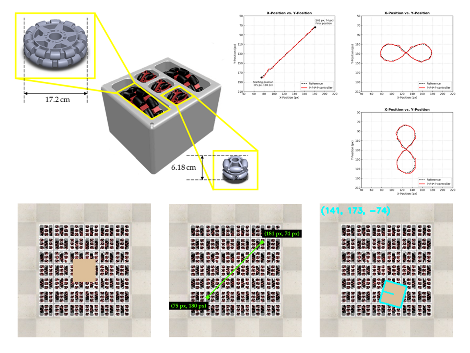
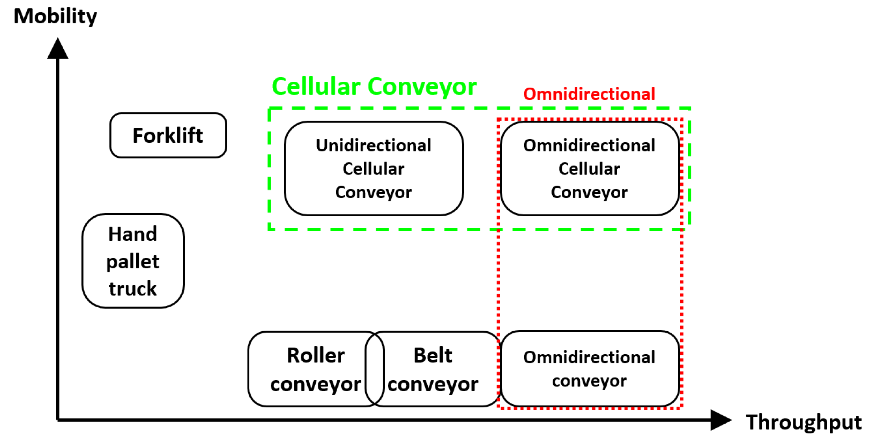
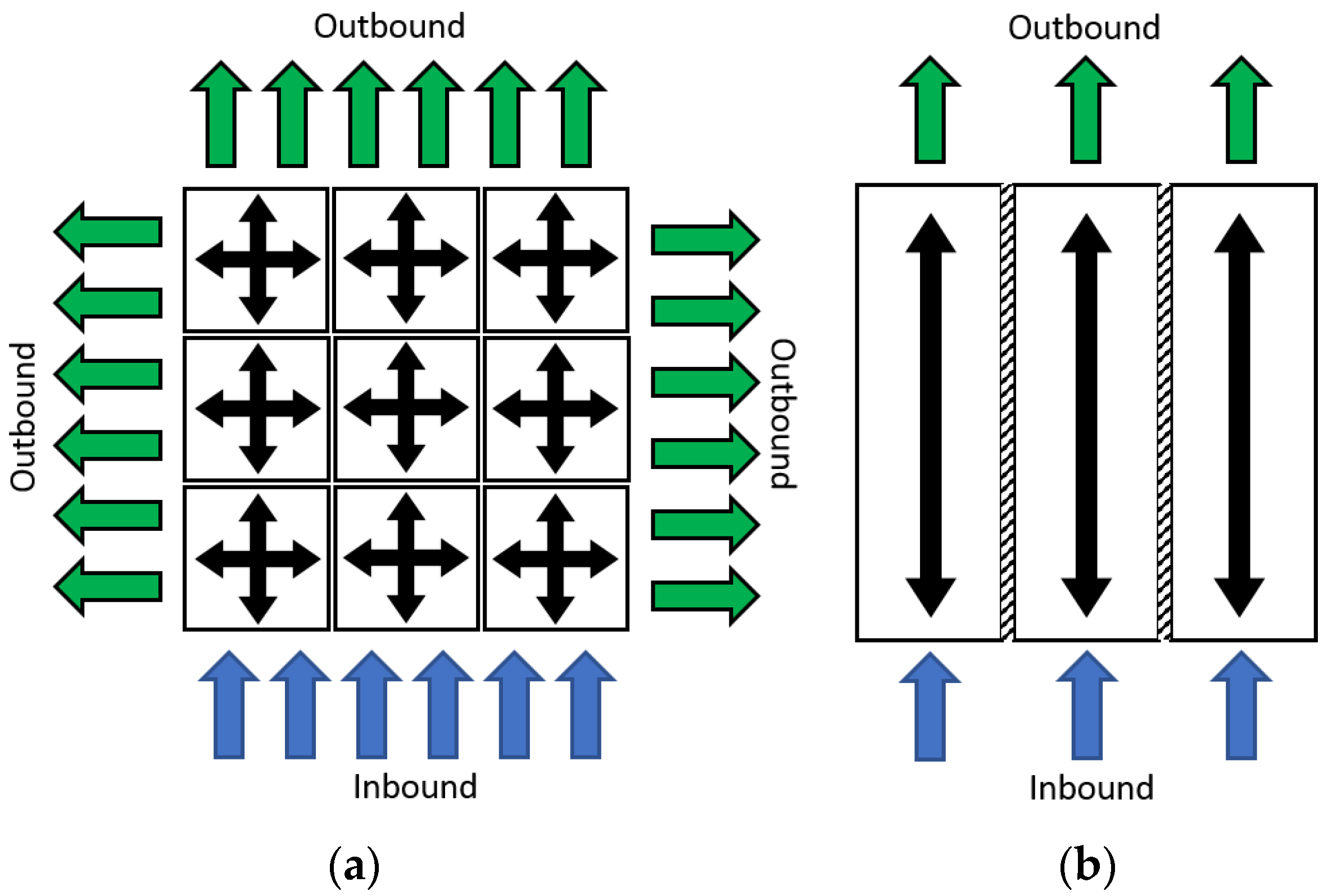
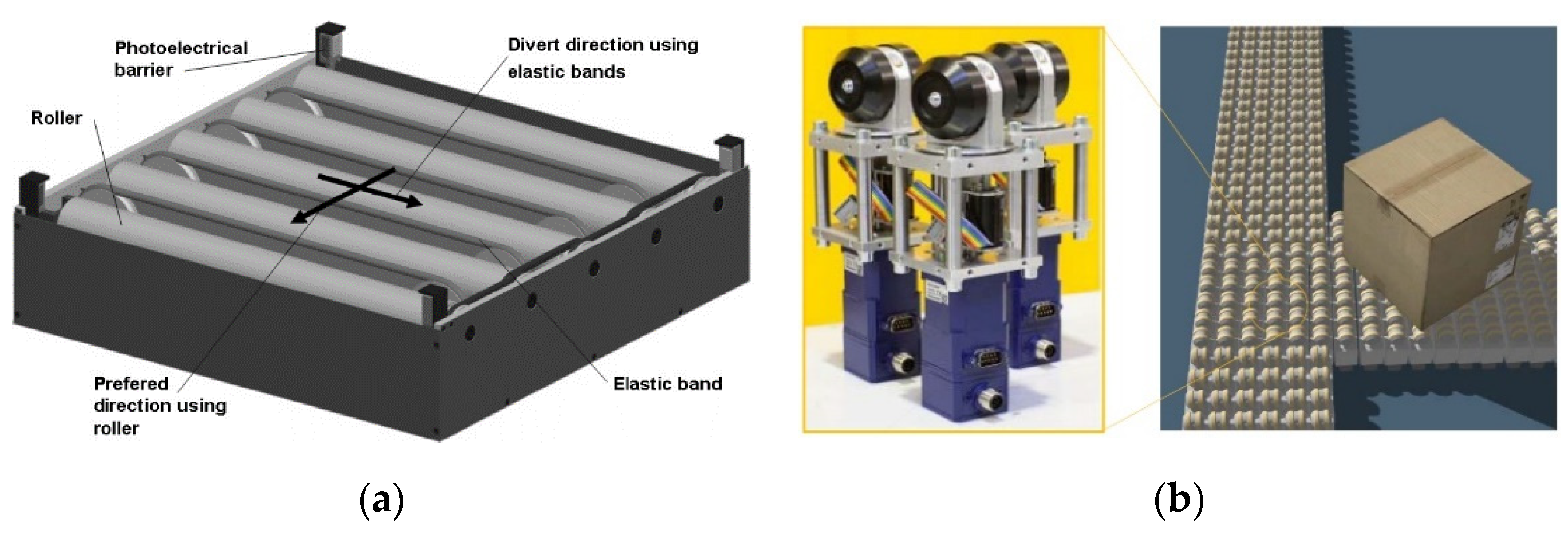
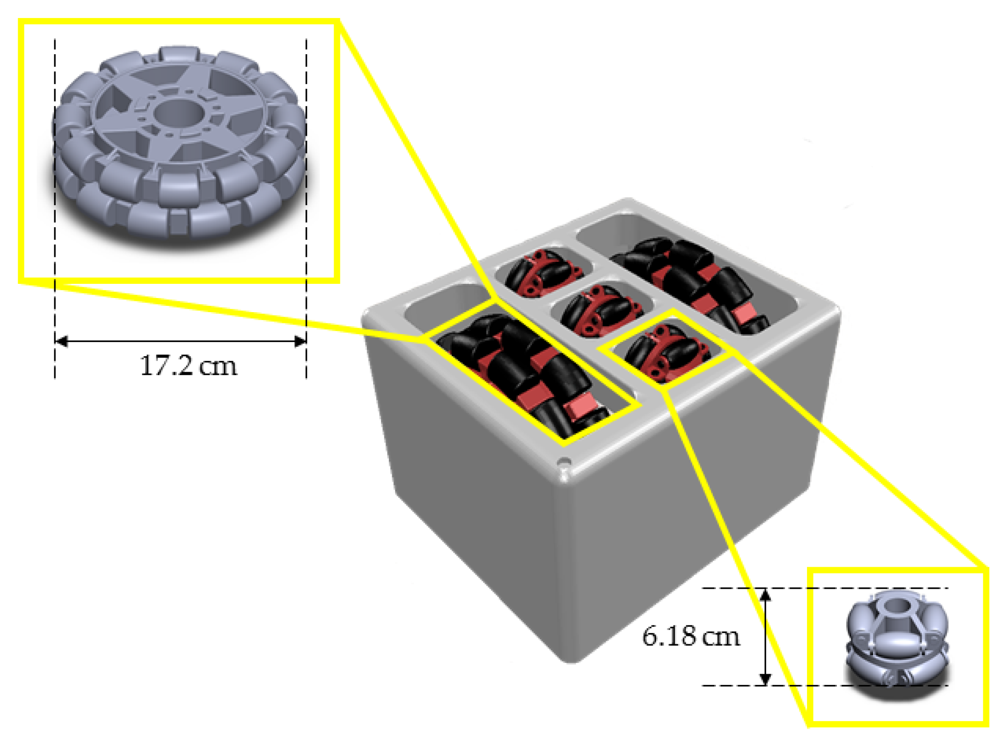
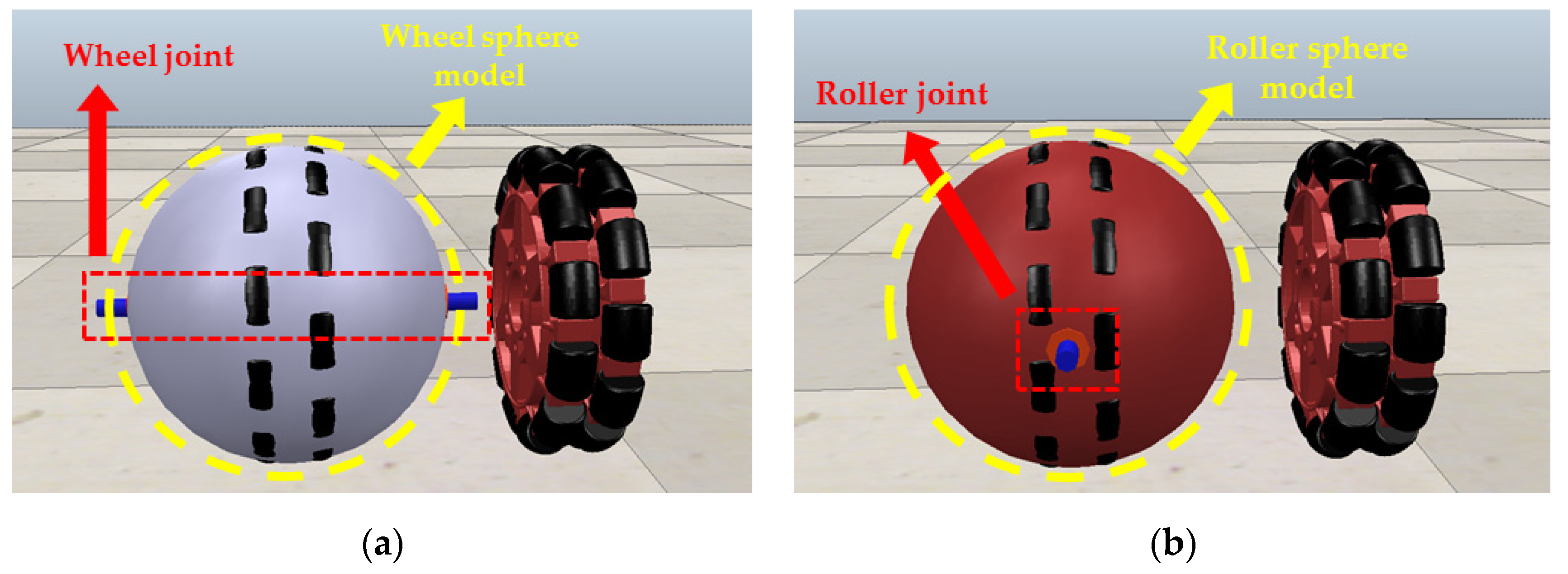
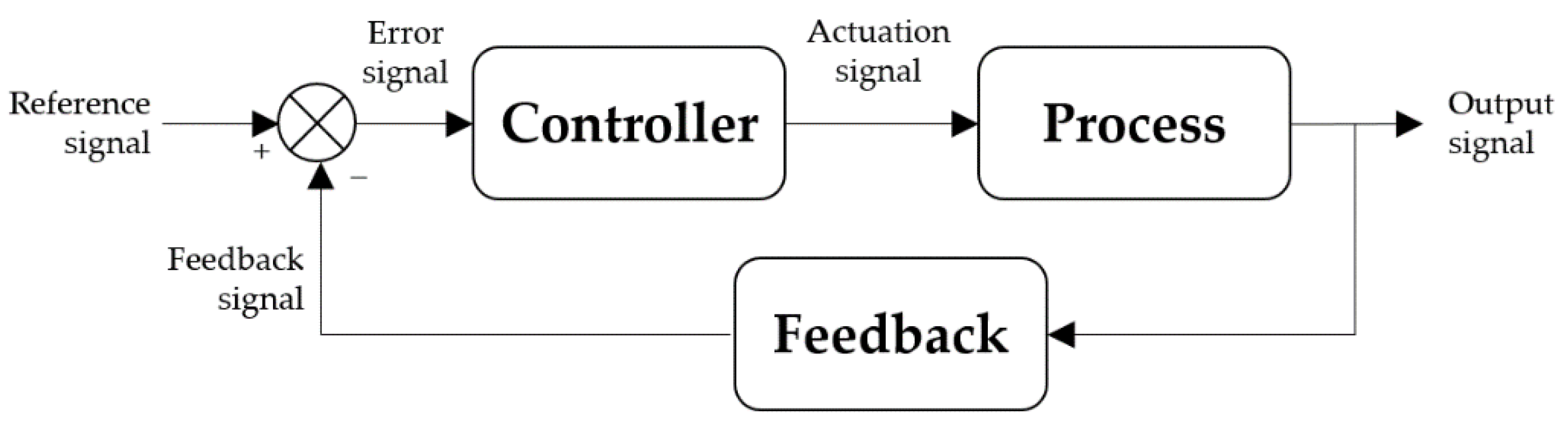
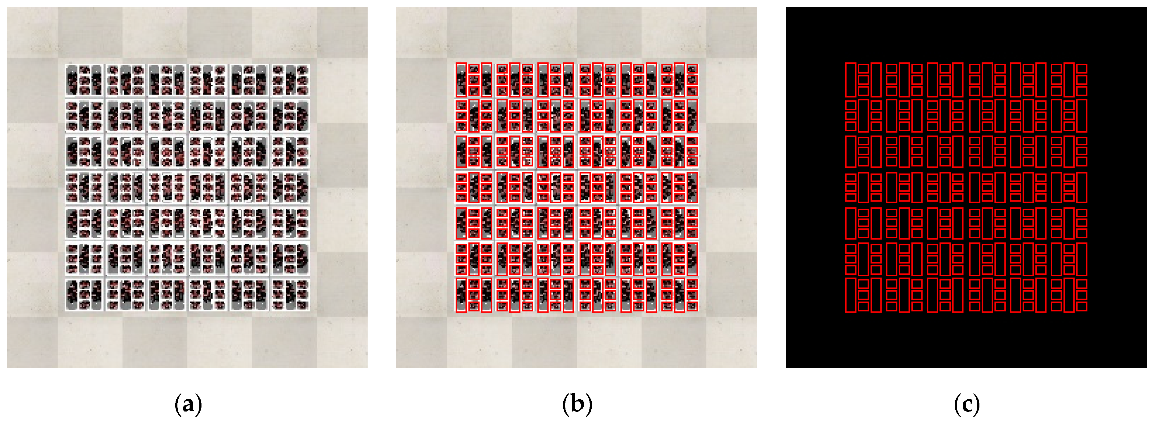
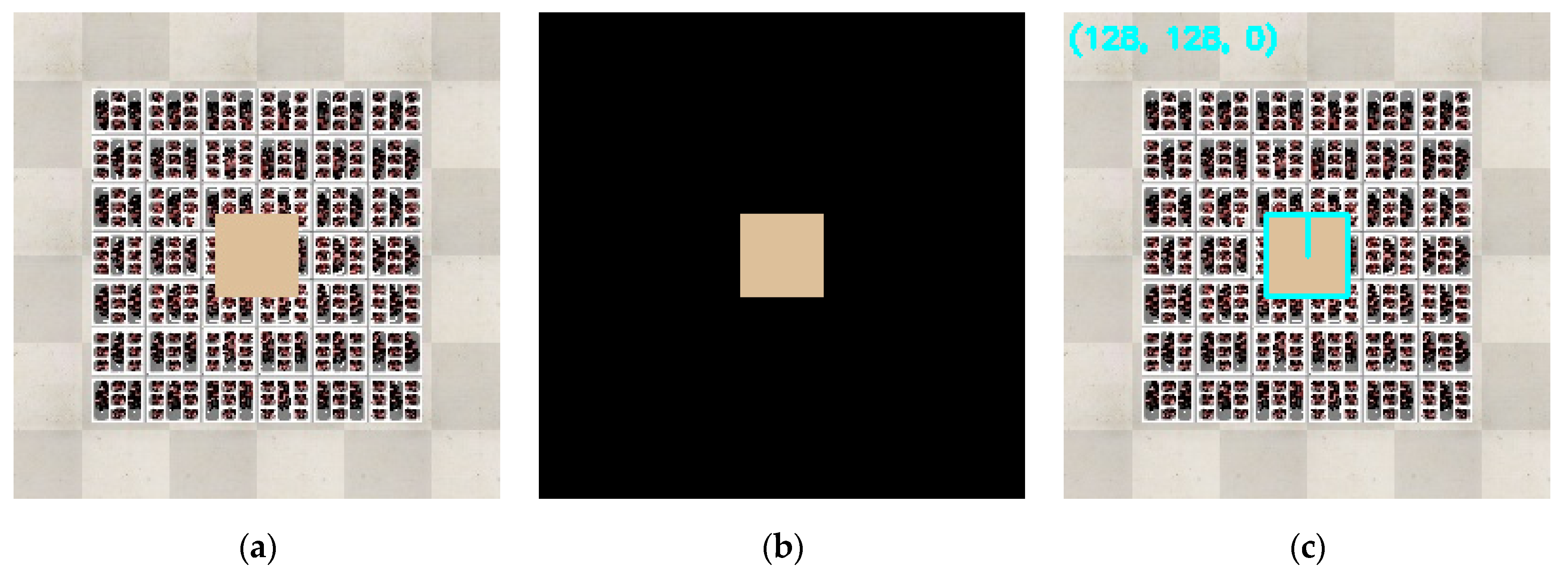
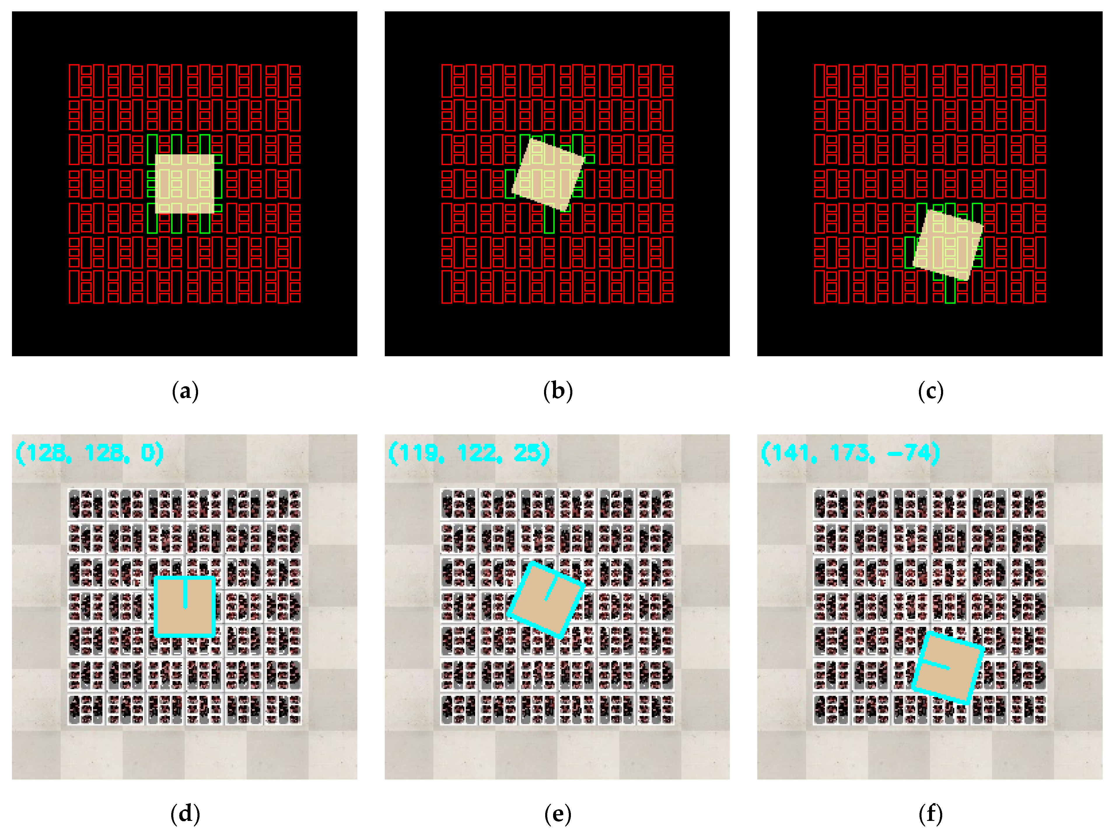
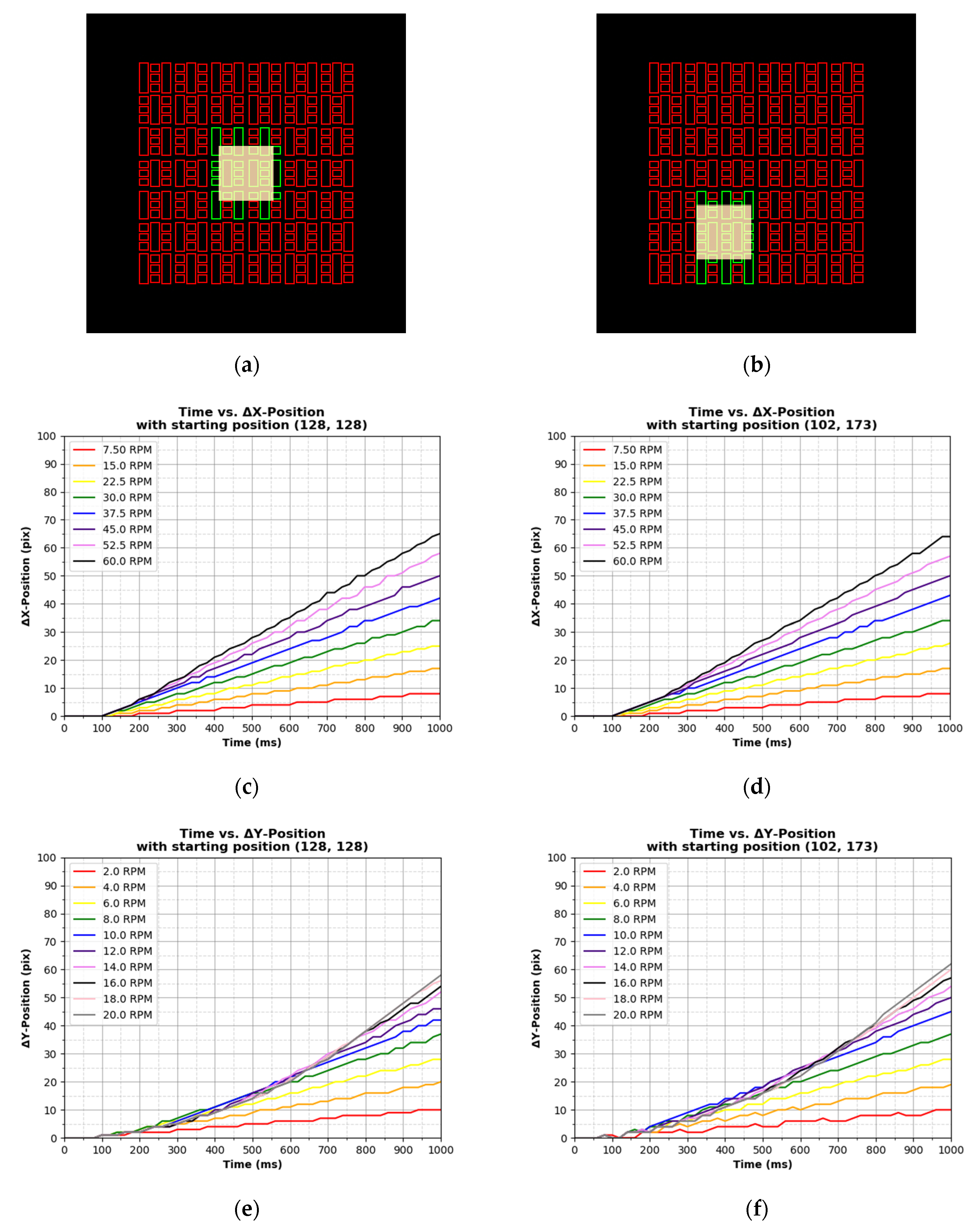
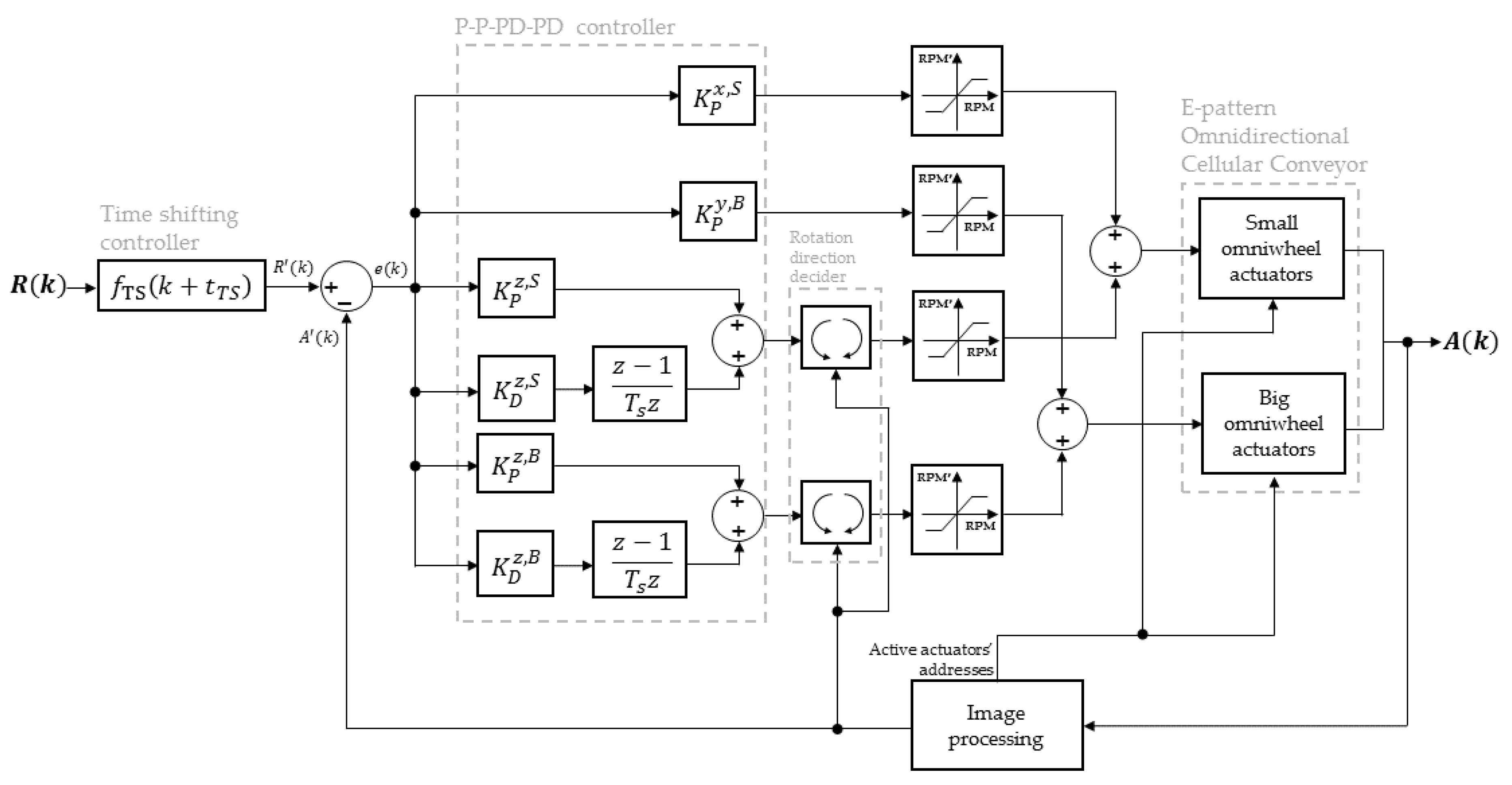
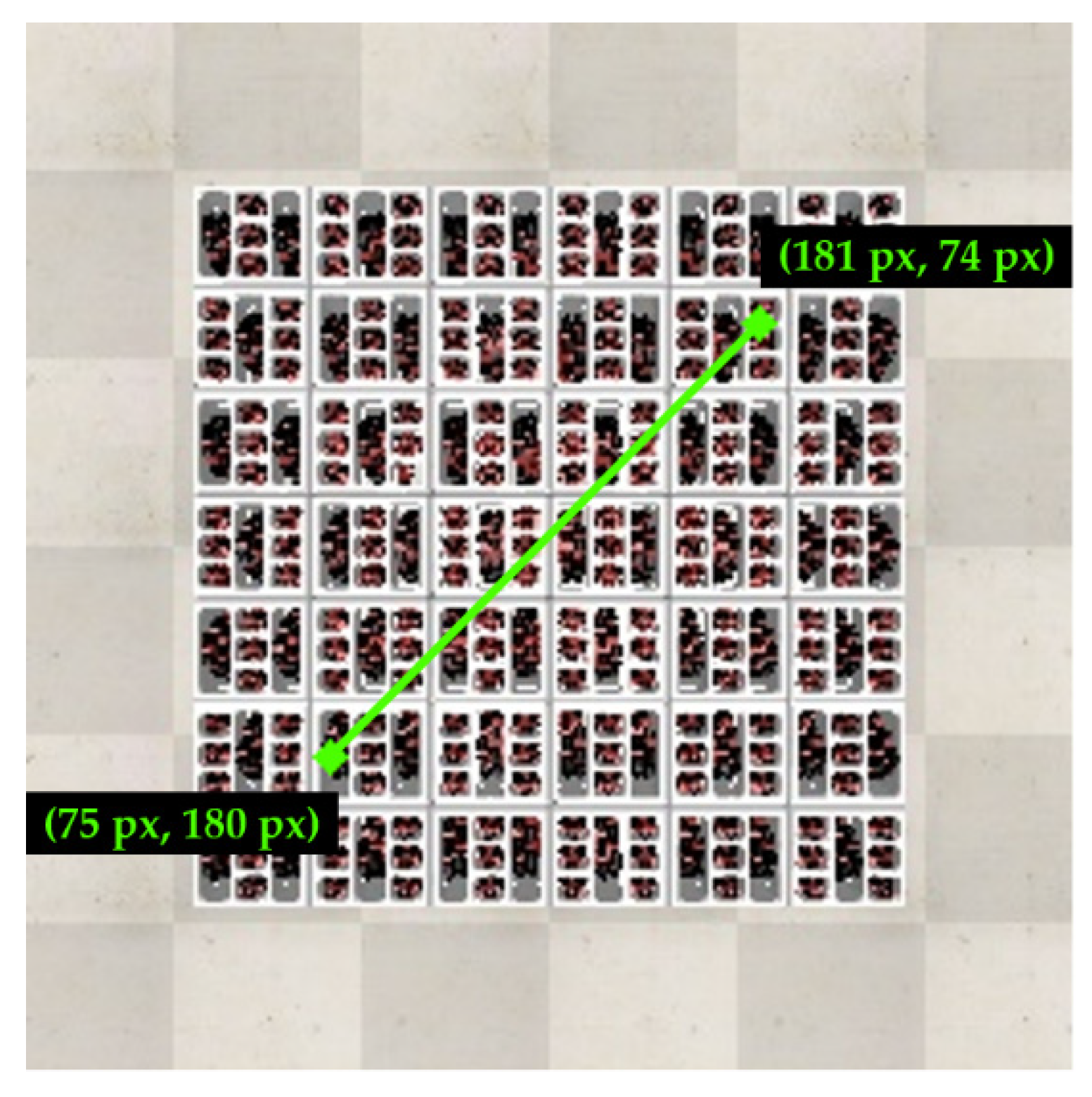
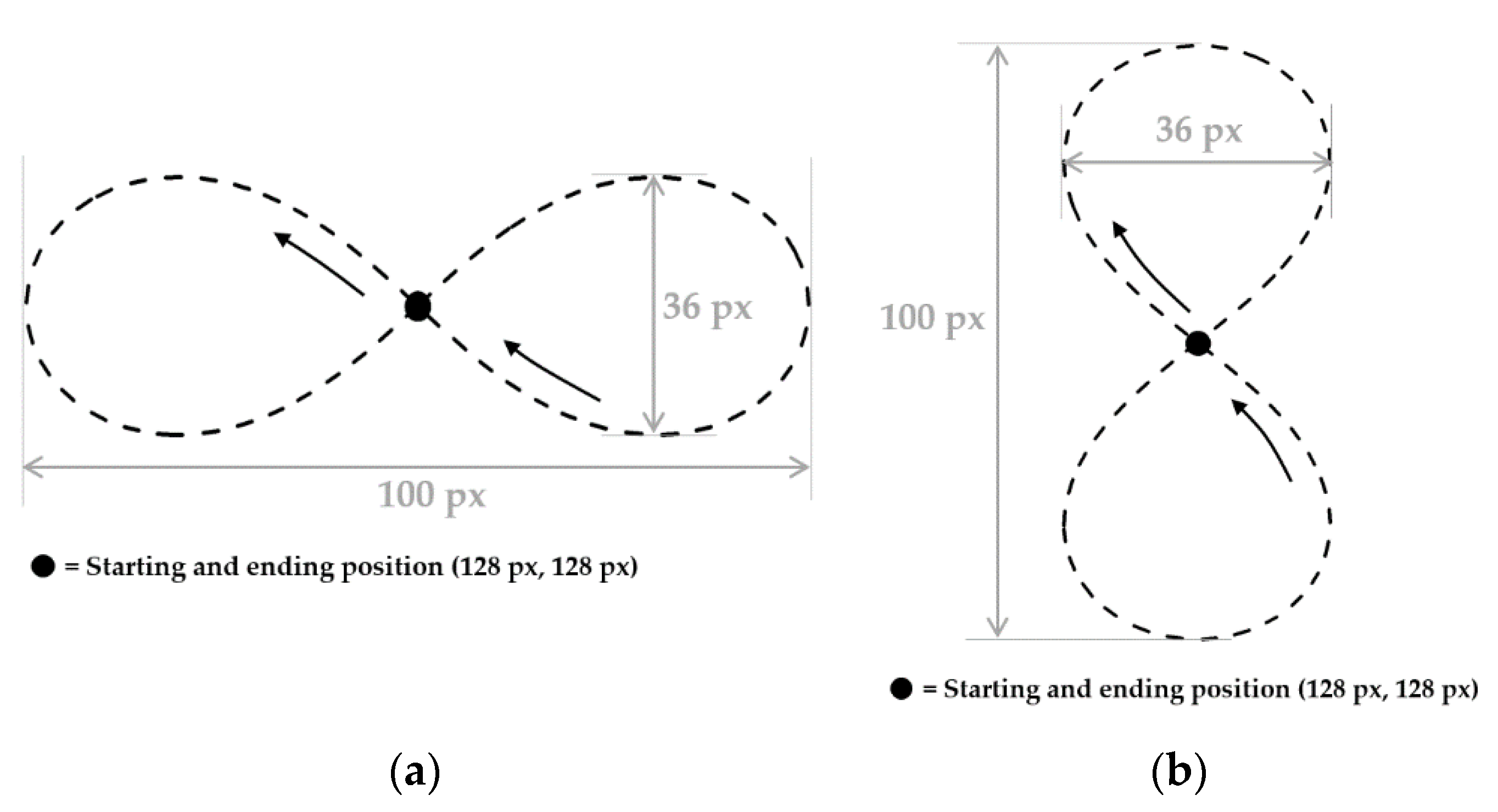
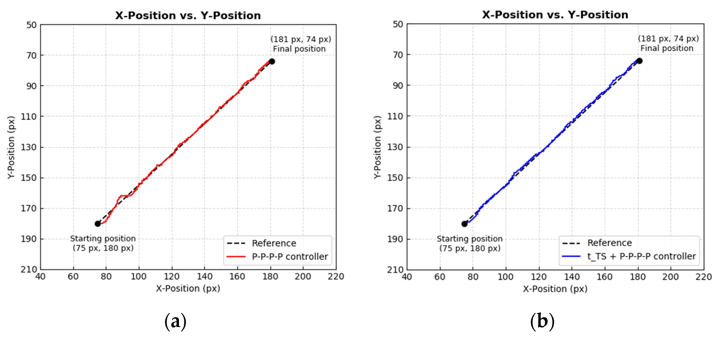
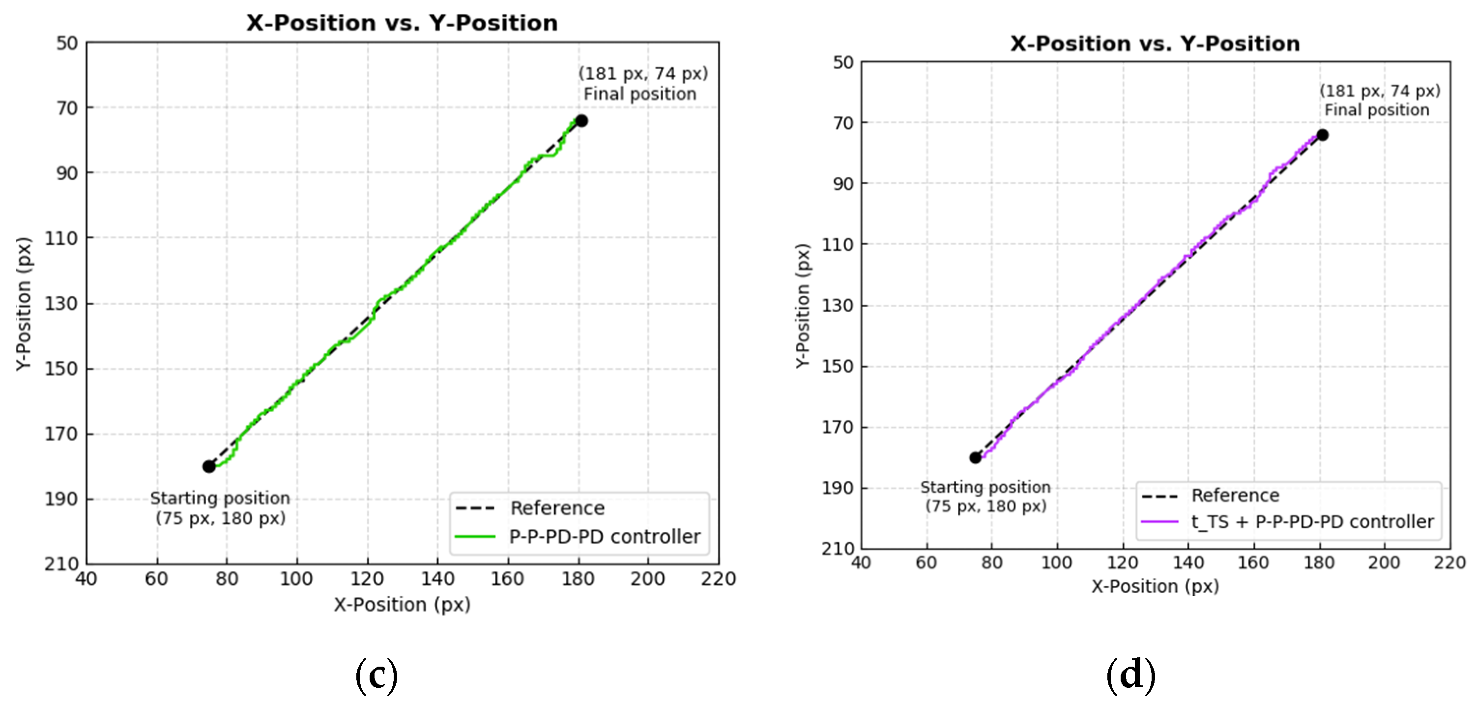
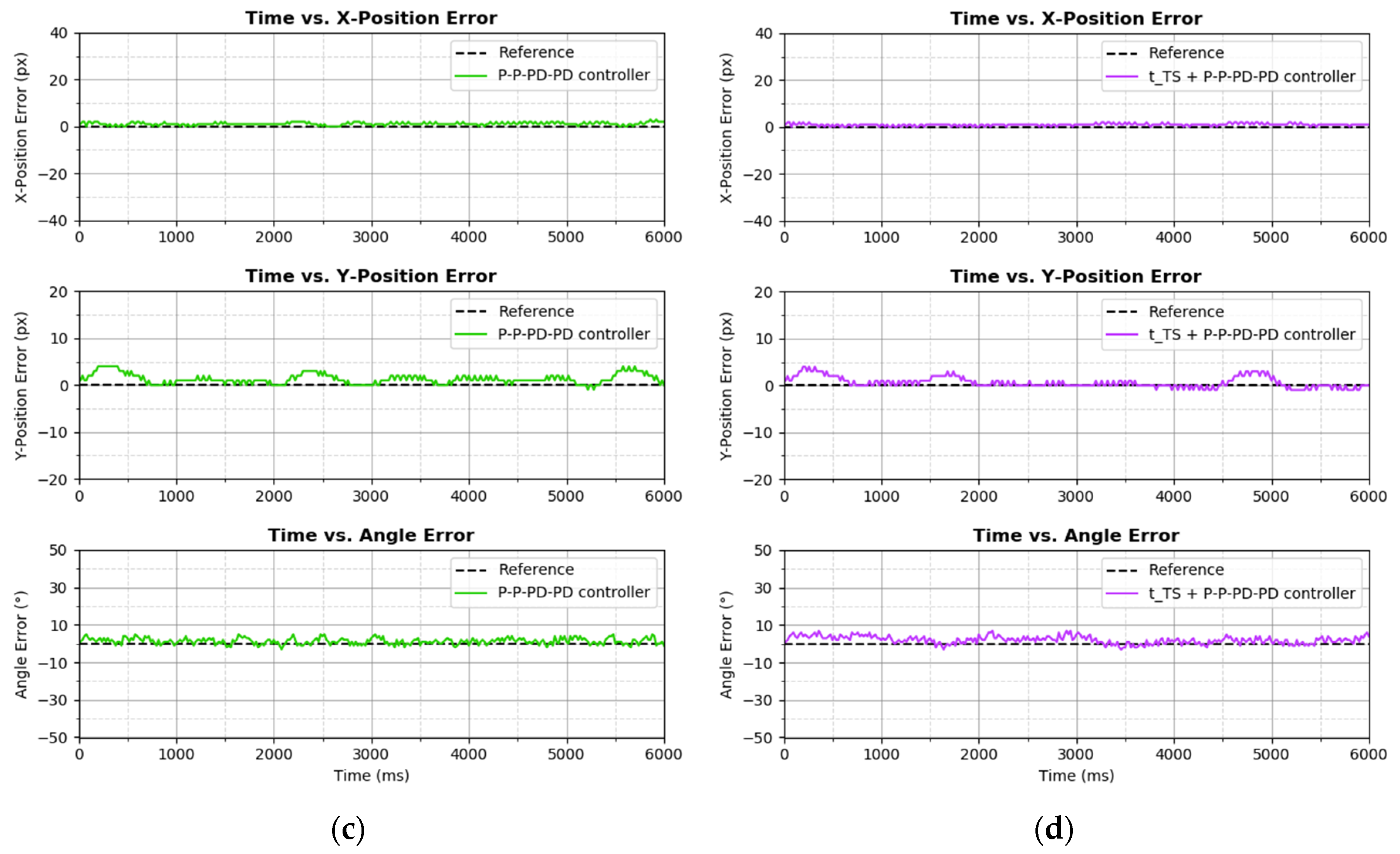
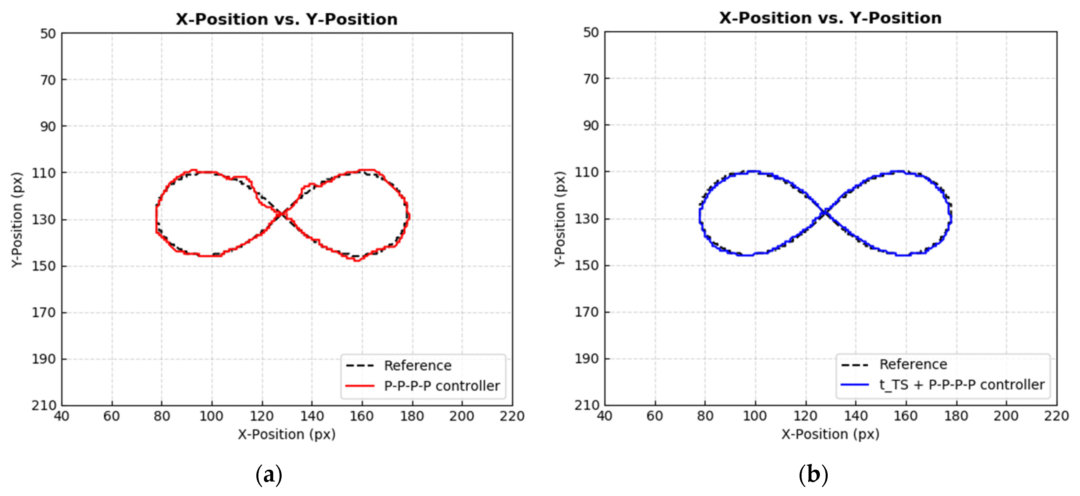
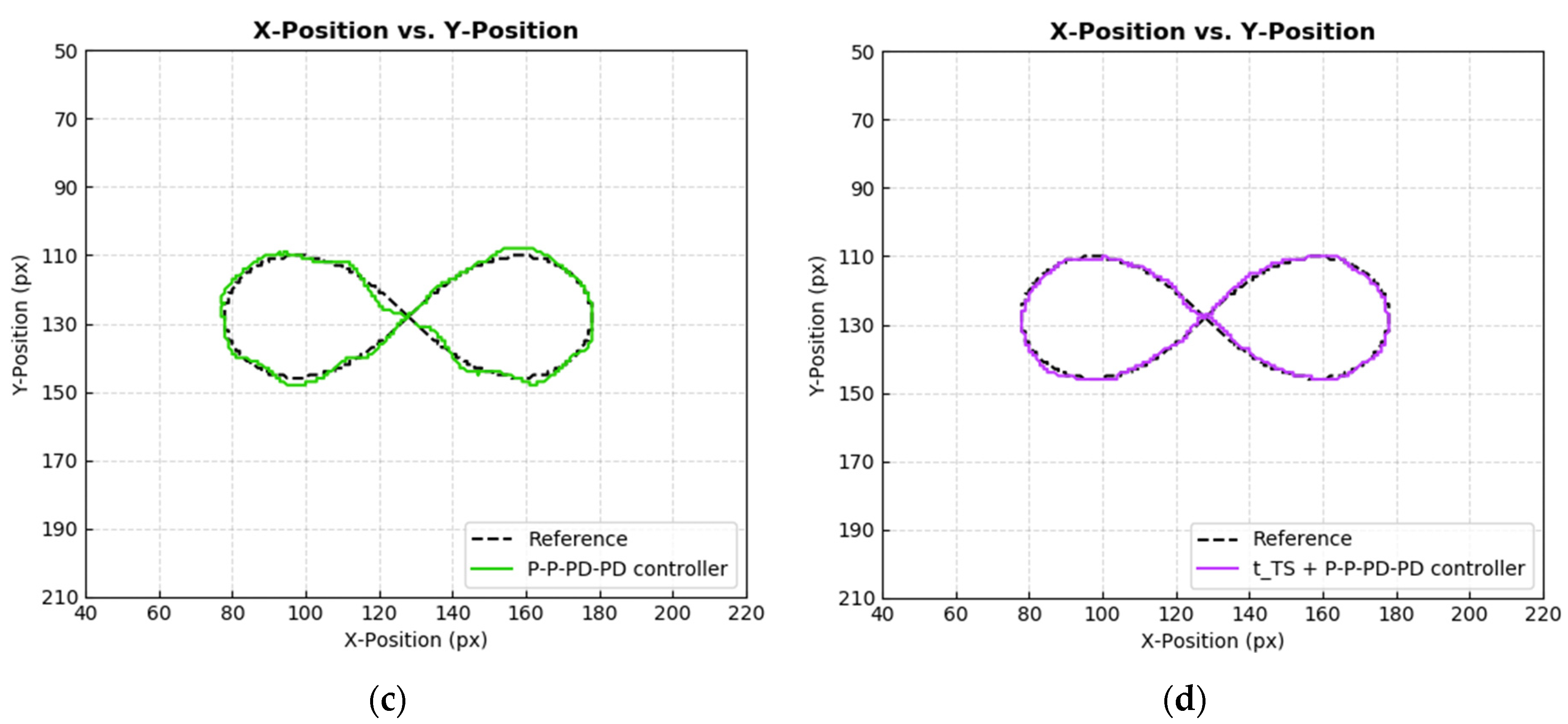
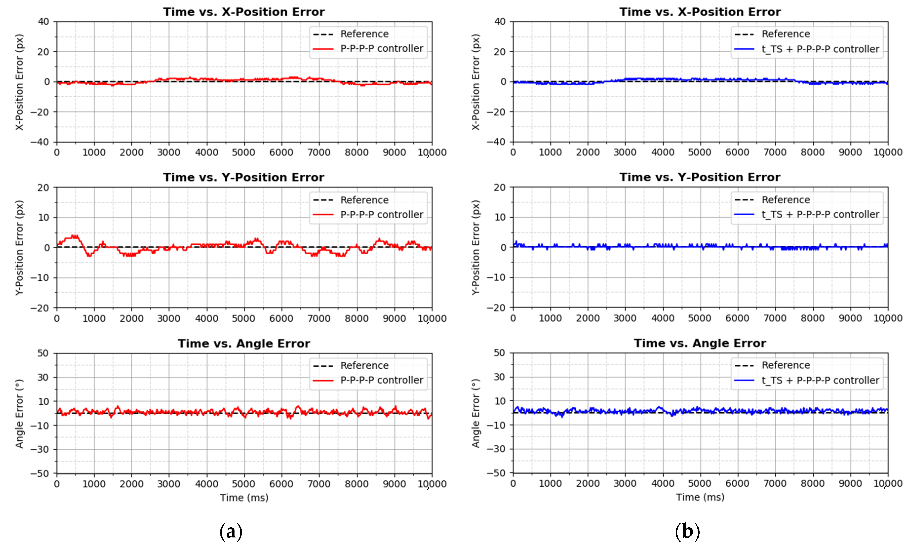
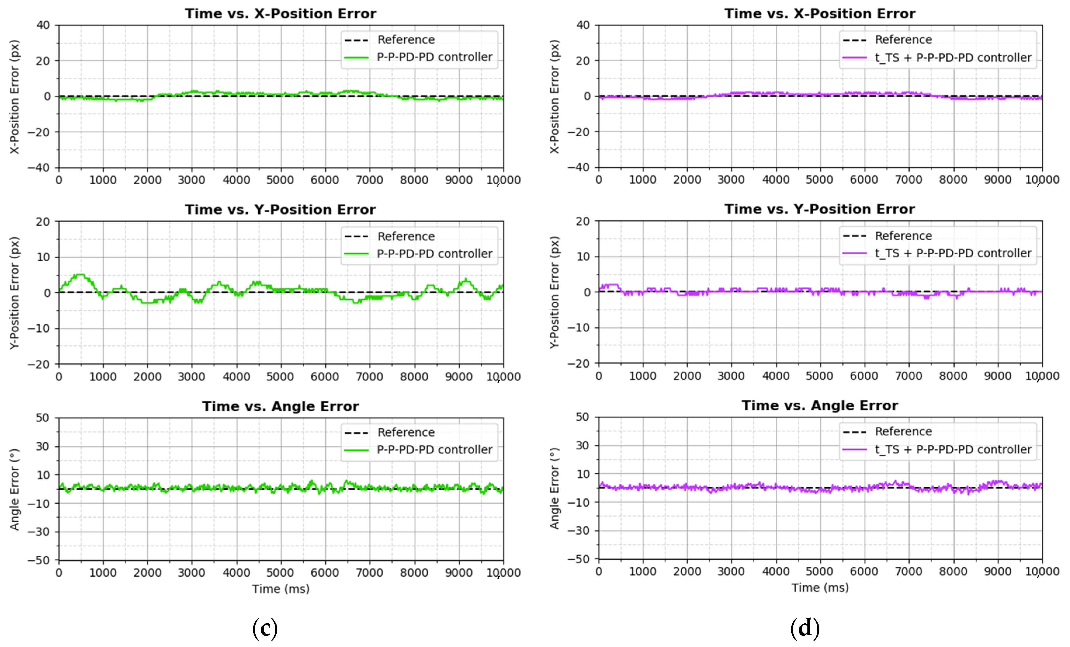
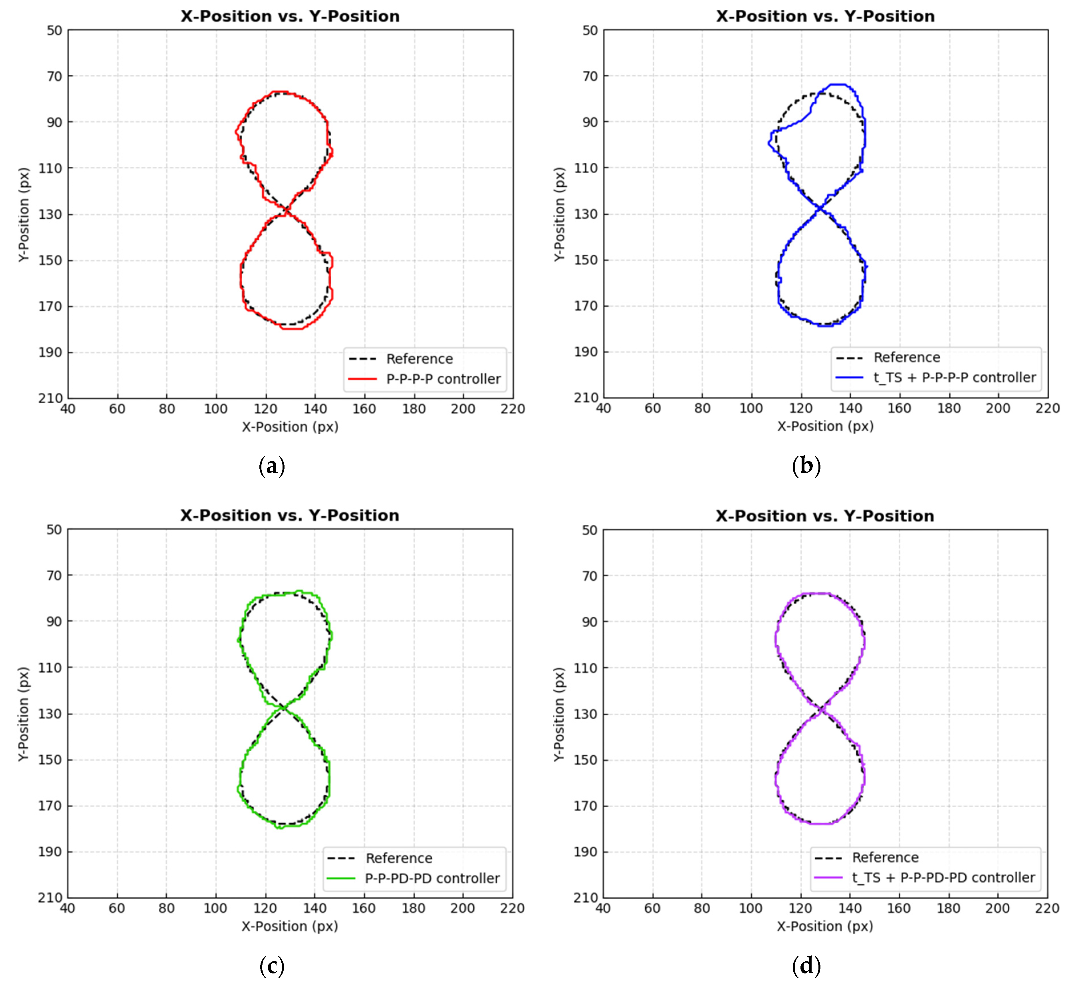
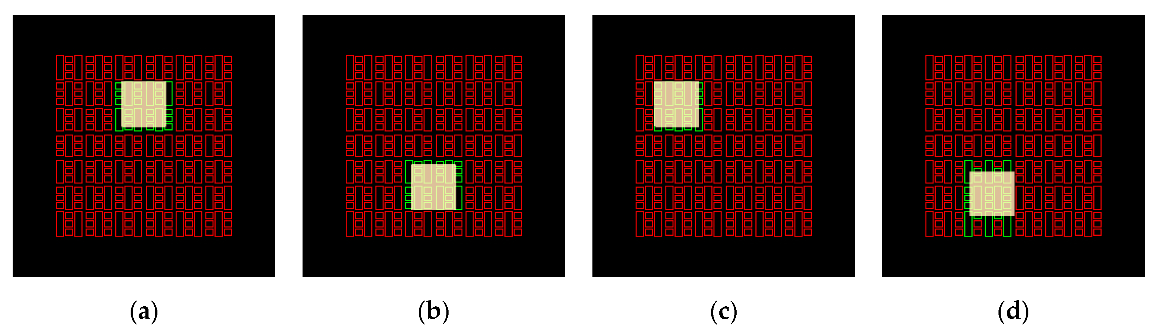
Table 1.
Parameters of each controller.
| Controllers | Parameters | ||||||
|---|---|---|---|---|---|---|---|
| P–P–P–P controller | 8.5 | 7.5 | 6.0 | — | 5.3 | — | — |
| + P–P–P–P controller | 3.5 | 2.1 | 1.0 | — | 0.3 | — | 100 |
| P–P–PD–PD controller | 8.5 | 7.5 | 6.0 | 90 | 5.3 | 100 | — |
| + P–P–PD–PD controller | 3.5 | 2.1 | 1.0 | 90 | 0.3 | 100 | 100 |
Table 2.
IAEs and ISEs by each controller in tracking of diagonal-shaped trajectory.
| X-Position | Y-Position | Angle | ||||
|---|---|---|---|---|---|---|
| IAE | ISE | IAE | ISE | IAE | ISE | |
| P–P–P–P controller | 352 | 518 | 350 | 742 | 572 | 1676 |
| + P–P–P–P controller | 326 | 470 | 145 * | 187 * | 759 | 3023 |
| P–P–PD–PD controller | 345 | 507 | 397 | 861 | 512 * | 1344 * |
| + P–P–PD–PD controller | 292 * | 364 * | 253 | 505 | 717 | 2535 |
* Lowest within the column.
Table 3.
IAEs and ISEs by each controller in tracking of ∞-shaped trajectory.
| X-Position | Y-Position | Angle | ||||
|---|---|---|---|---|---|---|
| IAE | ISE | IAE | ISE | IAE | ISE | |
| P–P–P–P controller | 688 | 1174 | 587 | 1135 | 781 | 2007 |
| + P–P–P–P controller | 598 | 874 * | 100 * | 102 * | 804 | 1958 |
| P–P–PD–PD controller | 720 | 1276 | 719 | 1649 | 727 * | 1701 * |
| + P–P–PD–PD controller | 600 * | 898 | 215 | 253 | 744 | 1756 |
* Lowest within the column.
Table 4.
IAEs and ISEs by each controller in tracking of 8-shaped trajectory.
| X-Position | Y-Position | Angle | ||||
|---|---|---|---|---|---|---|
| IAE | ISE | IAE | ISE | IAE | ISE | |
| P–P–P–P controller | 583 | 955 | 869 | 2555 | 775 * | 2013 |
| + P–P–P–P controller | 456 | 780 | 964 | 3858 | 3006 | 22,268 |
| P–P–PD–PD controller | 543 | 871 | 934 | 3002 | 778 | 1930 * |
| + P–P–PD–PD controller | 420 * | 536 * | 242 * | 312 * | 1820 | 8012 |
* Lowest within the column.
Publisher’s Note: MDPI stays neutral with regard to jurisdictional claims in published maps and institutional affiliations. |
© 2021 by the authors. Licensee MDPI, Basel, Switzerland. This article is an open access article distributed under the terms and conditions of the Creative Commons Attribution (CC BY) license (http://creativecommons.org/licenses/by/4.0/).
Share and Cite
MDPI and ACS Style
Keek, J.S.; Loh, S.L.; Chong, S.H. Design and Control System Setup of an E-Pattern Omniwheeled Cellular Conveyor. Machines 2021, 9, 43. https://0-doi-org.brum.beds.ac.uk/10.3390/machines9020043
AMA Style
Keek JS, Loh SL, Chong SH. Design and Control System Setup of an E-Pattern Omniwheeled Cellular Conveyor. Machines. 2021; 9(2):43. https://0-doi-org.brum.beds.ac.uk/10.3390/machines9020043
Chicago/Turabian StyleKeek, Joe Siang, Ser Lee Loh, and Shin Horng Chong. 2021. "Design and Control System Setup of an E-Pattern Omniwheeled Cellular Conveyor" Machines 9, no. 2: 43. https://0-doi-org.brum.beds.ac.uk/10.3390/machines9020043
Note that from the first issue of 2016, this journal uses article numbers instead of page numbers. See further details here.