
Design of Nonlinear Control of Gas Turbine Engine Based on Constant Eigenvectors †


1
Department of Computer Science and Robotics, Ufa State Aviation Technical University, 450008 Ufa, Russia
2
Department of Information Technologies, Sochi State University, 354008 Sochi, Russia
*
Author to whom correspondence should be addressed.
†
This paper is an extended version of Valeev, S.; Kondratyeva, N. Design of Nonlinear Multi-Mode Controller for Gas Turbine Engine in State Space Based on Algorithmic Approach. In Proceedings of the 2020 International Russian Automation Conference (RusAutoCon 2020), Sochi, Russia, 6–12 September 2020; pp. 1053–1057.
Machines 2021, 9(3), 49; https://0-doi-org.brum.beds.ac.uk/10.3390/machines9030049
Submission received: 29 January 2021
/
Revised: 14 February 2021
/
Accepted: 22 February 2021
/
Published: 25 February 2021
(This article belongs to the Special Issue Mechatronic System for Automatic Control)
Abstract
:A gas turbine engine represents a complex dynamic control object. Its characteristics change depending on the state of the environment and the regimes of its operation. This paper discusses an algorithmic approach to the design of a nonlinear controller, based on the concept of constant eigenvectors and analytical design of the control system. The proposed design method makes it possible to ensure the stability and the required quality of transient processes at different acceleration modes. In this case, the constancy of the matrix of the canonical basis of the closed-loop control system is assumed, which guarantees stability. The design of a neural network dynamic model of a gas turbine engine based on a neural network approximator with one input and multiple outputs is considered. An example of the design of a nonlinear controller for a gas turbine engine is considered, the neural network model of which is given in the state space. The application of neural network approximation of controller coefficients is presented.
1. Introduction
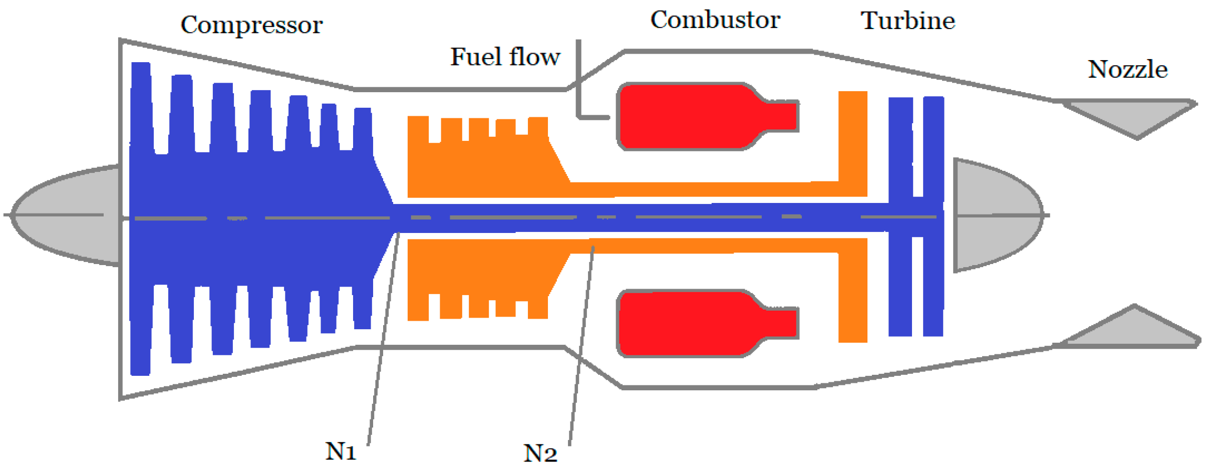
A gas turbine engine is a complex heat machine in which numerous subsystems serve the main purpose of creating jet thrust for aircraft movement [1]. A gas turbine engine includes the following main components: inlet, compressor, combustion chamber, turbine, and nozzle [2]. Compressed air is mixed with fuel and ignited in the combustor chamber [3]. The turbine extracts thermal energy from the hot air to drive the compressor and to create thrust for moving aircraft [4].
A control system is used to ensure efficient engine operation. The main tasks of the control system of a gas turbine engine are to ensure the efficiency of the power plant in various regimes [5], and to provide the safe running of the processes of generating thrust [6], taking into account technological limitations [7,8].
Depending on the purpose and design features, gas turbine engines can be assigned to different types [4]. For example, Figure 1 shows a simplified diagram of a twin-shaft jet engine, where N1 is low pressure compressor speed and N2 is high pressure compressor speed. These parameters determine the performance of this complex control object [9,10].
To solve the problem of control of multidimensional nonlinear dynamic objects, the method of decentralized control has become widespread, in which the automatic control system is divided into a number of separate (autonomous) subsystems [11]. Each of these subsystems measures one of the controlled coordinates, compares it with the reference value (command), and generates a control action coming to the corresponding input of the control object [12].
At various stages of the lifecycle of the control system, models of varying complexity are used: Element-by-element [13], multiregime [14], and point models [15].
The development of nonlinear control systems for unsteady engine operation is based on the use of the direct Lyapunov method. The procedure for constructing the required Lyapunov function, taking into account the nature of the mathematical description of the gas turbine engine, is a nontrivial problem [16].
Methods based on the assumption of linearity of the gas turbine engine characteristics in a small vicinity of the operating mode are usually used as methods for synthesizing control subsystems. This assumption is made to simplify the synthesis procedure for automatic control systems and allows one to synthesize controllers that provide the required quality of transient processes in the stabilization modes of automatic control systems [13,16].
At the design stage of gas turbine engine control systems, piecewise linear models are used to take into account the nonlinear nature of the engine characteristics and the dynamic properties of the engine in different regimes using a set of linear models. Nonlinear static lines of the operating regime and linear models in the state space serve as a basis for constructing models of this class.
Static characteristics are presented as a set of piecewise linear dependencies at points selected by the developer. At the selected points of the operating mode, the dynamic properties of the gas turbine engine are described using linear models in the form of transfer functions or in the form of linear dynamic models in the state space [13].
When constructing a multiregime controller, piecewise linear interpolation is used to stitch the values of the parameters of linear controllers obtained at the previous stage of design [13,17,18].
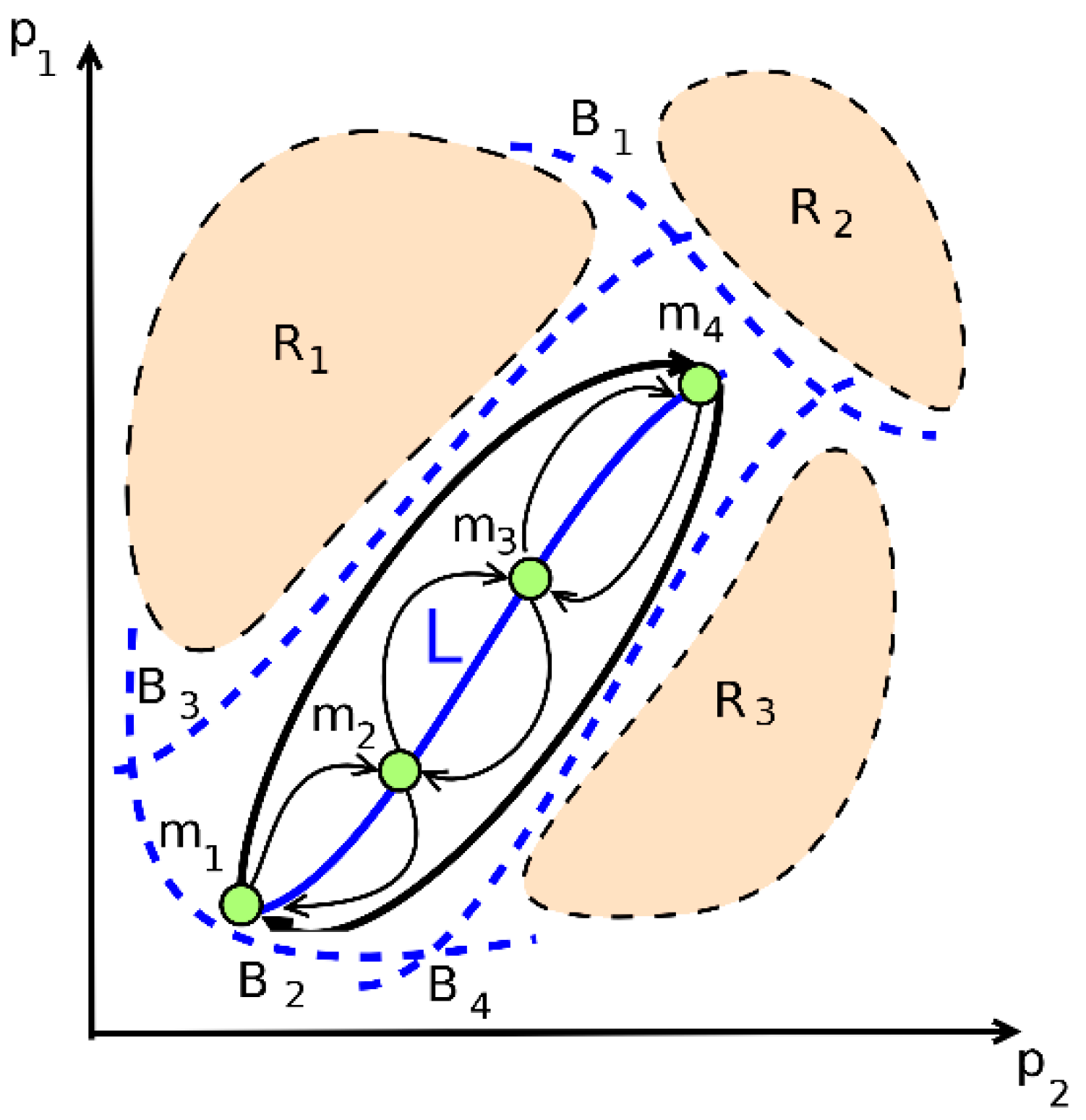
For compressors and turbines, the features can be presented in the form of performance “maps” that describe the full envelope of behavior for that system. A generalized compressor map of a gas turbine engine is presented in Figure 2. The detailed description can be found in [5,6].
Figure 2 shows schematically the change in compressor characteristics in transient modes, where:
- P1 is compressor average pressure ratio;
- P2 is inlet corrected mass flow rate;
- R1 is compressor surge region;
- R2 is turbine gas temperature limit region;
- R3 is flameout region;
- mi are points on engine steady running line L;
- m1–m4 is the trajectory during acceleration;
- m4–m1 is the trajectory during deceleration;
- B1–B4 are the boundaries of stable operation of the compressor.
The task of the controller is to ensure the stable operation of the gas turbine engine, taking into account the specified limitations. The complexity of solving the design problem is associated with the significantly nonlinear nature of the characteristics of the gas turbine engine, depending on the operating regimes.
One of the approaches to the design of control algorithms for a gas turbine engine is the design of nonlinear multiregime controllers based on the description of the dynamic properties of the engine parameters in the state space. The advantages of this approach in the design of multiregime controllers include the possibility of taking into account nonlinearities of a dynamic model of the engine.
The design of an algorithm for controlling a dynamic object in a state space is usually understood as the problem of determining the structure and parameters of controllers that provide the specified spectral properties of closed-loop control system eigenvalues. The method is usually based on the choice of control in the form of feedback from state variables [19]. The presence of feedbacks ensures the required placement of the eigenvalues of the closed system on the complex plane. Moreover, the controller has a fairly simple structure [20]. The algorithmic complexity of this control algorithm depends linearly on the dimension of the input problem or the order of the control system [21].
2. Nonlinear Control Design Method Based on Constant Eigenvectors
At present, approaches of analysis and design of nonlinear control systems based on analytical methods are widely used [17,22]. These methods include, among others, the matrix methods of analysis and design of nonlinear systems, proposed in [23]. Common to these methods is the use of eigenvalues and constant eigenvectors when solving problems of analysis and design of automatic control systems. It is shown that if the eigenvectors of the linear part of the system are constant eigenvectors for the nonlinear part as well, then the eigenvalues of the nonlinear system are functions of its state variables. The assignment of eigenvalues or functions of the state variables of the control system guarantees the required character of transient processes. Constant eigenvectors together with eigenvalues determine the required estimates of the attraction domain of the control system [24]. When analyzing and designing control algorithms within the framework of this approach, it is necessary to determine all sets of constant eigenvectors of nonlinear homogeneous vector functions determined by the right-hand side of nonlinear differential equations of the control system.
When solving the problem of control design in the state space for a linear dynamic system, a controlled linear system with constant coefficients is considered:
A linear feedback is chosen so that the eigenvalues of the closed-loop system
i.e., the roots of the characteristic equation, are equal to a given set of values {λ}.
When designing control in the state space, the following main types of control situations are distinguished:
- Search for scalar control or vector control;
- Design control with complete or incomplete information;
- Control with complete or incomplete controllability of the eigenvalues of the closed system. Different algorithmic approaches are used depending on the type of control situation.
Let us further consider the main provisions of the analysis and design of nonlinear systems based on constant eigenvectors, the concept of which was introduced in [23,24].
If for a linear system of differential equations the linear transformation is applied
where mi is eigenvector, then the solution of System (1) will have the form
where is the diagonal matrix.
For a nonlinear system of the form
by analogy with linear systems, the equation for the eigenvalues and eigenvectors can be written in the following form:
Then, substituting the nonlinear transformation
into (4), we get
From (5) we find a solution in the following form
Due to the term in (6), it is inadmissible to evaluate the stability of System (4) only by the roots of the characteristic equation
since in Equation (6) the matrix
If for A (x), but that is, the matrix M (x) is composed of constant vectors, then , and the solution to System (6) has the form:
Let us further consider the case when for the nonlinear System (4) the matrix of the canonical basis M = const. We expand the right-hand side of System (4) into a Taylor series at a given point:
where ; are i-th order terms with respect to x (i = 2 ÷ k); n is the system order.
Let us assume that the following condition is true:
i.e., the eigenvectors of the linear part of the nonlinear System (9) and the eigenvectors of the homogeneous right-hand side of System (9) coincide.
Next, it is needed to find the constant matrix of the canonical basis M with the help of which the following transformation is performed:
Or
where Gs (x) is eigenvalue (function of system coordinates) for A (x).
Since is a linear transformation (where M is the matrix of the canonical basis), the stability of System (12) means the stability of System (4).
3. Neural Network Dynamic Model of a Gas Turbine Engine
To solve problems of design of control algorithms for a gas turbine engine, piecewise linear dynamic models are widely used, given in the form of a set of point linear models for a set of points on the steady state line [17]. Application of linear models for the design of control at a given point makes it possible to simplify the design procedure. The design of the controller is carried out for each given point of the operating regime. When changing the operating regime of the gas turbine engine, i.e., when passing from one point of the operating regime to another, it is assumed that additional disturbances do not arise, i.e., the required quality of control processes is ensured. However, in acceleration regimes, i.e., regimes in which the characteristics of the engine change as much as possible and the line of motion of the operating point passes in the vicinity of the regions of specified constraints on the change in engine parameters, the problem of developing a nonlinear controller arises.
To ensure the functioning of a set of models as a whole in a given range of changes in the operating regimes of a gas turbine engine, the problem of interpolating the coefficients of piecewise linear dynamic models is solved:
where:
- , ;
- are values of the vectors of variables x, u, y at static (steady-state) operating regimes of a gas turbine engine (i = 1, …, 4);
- is the vector of state variables (which are understood as the rotational speeds of the low and high pressure compressors of the gas turbine engine, respectively);
- is the vector of control actions (fuel consumption and jet nozzle cross-sectional area);
- is the vector of controlled variables (air pressure behind the compressor, gas pressure and temperature behind the turbine);
- is a parameter that determines the choice of the point of the i-th operating mode (or, respectively, the i-th piecewise linear model);
- are relative (dimensionless) values of variables N1 and N2.
Considering that the parameter η is a function of continuous variables, the gas turbine engine model can be represented as a system of nonlinear differential equations:
In [25,26,27,28,29], it was shown that neural networks are universal approximators, i.e., these allow for solving the problem of approximating a function with a given accuracy on the trained input and output set of values. Currently, neural networks are widely applied for control of dynamic objects [30,31], modeling [32,33], adaptive control [34], and predictive control [35,36].
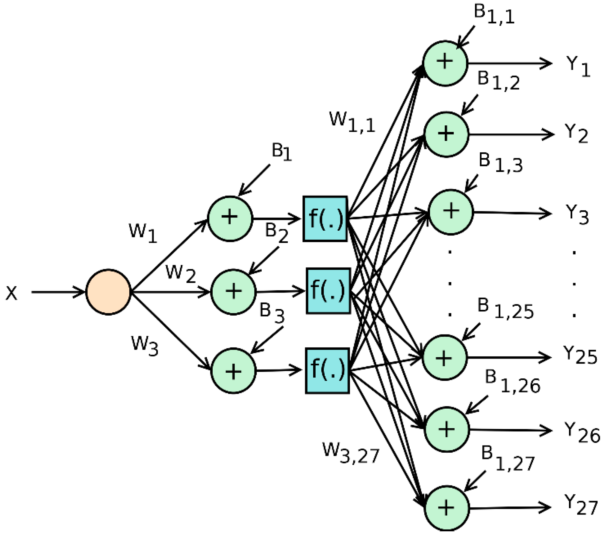
The neural network shown in Figure 3 approximates a set of nonlinear functions with a given accuracy on a training set of values. A characteristic feature of this approximator is the presence of one input and several outputs (single input–multiple output (SIMO)-approximator).
When solving the problem of interpolating the coefficients of a set of linear models using neural network technology, a nonlinear multiregime dynamic engine model can be represented in the following form:
where:
- fi (x) is neuron activation function (scalar function of vector argument);
- are configurable neural network weights;
- are biases in separate layers of the neural network, , where n is the number of neurons in the hidden layer.
The accuracy of the dynamic nonlinear model of a gas turbine engine (15) in our case depends on the number of neurons in the hidden layer [26,37]. An obvious advantage of this approach is the ability to provide the required accuracy of interpolation of coefficients and variables, since it is known that neural networks are universal approximators.
As we see from (15), the dynamic model of the engine is described by a set of nonlinear equations and nonlinear differential equations. This model is a simplified nonlinear model of the operation of the engine for a set of specified regimes and combines all available information about the dynamic properties of the engine in a given range of changes in the regimes of its operation.
4. Algorithm for Design of a Nonlinear Control System for Gas Turbine Engine
Let the set of linear dynamic models of the gas turbine engine be given in the state space that describe, with a given accuracy, the gas turbine engine as a dynamic control object on a set of regimes of its operation. We assume that each linear model corresponds to the i-th basic operating point on the steady-state line L (see Figure 2).
Let us state the problem of designing a nonlinear controller that ensures stable operation and the given quality of operation of the gas turbine engine in the entire range of operating regimes.
Consider an algorithmic method for the design of nonlinear control for the discussed class of nonlinear control systems. The generalized scheme of the nonlinear control design algorithm is shown in Figure 4.
The design algorithm for a nonlinear controller includes the following main steps.
Step 1. At the first step, the set of linear dynamic models is formed from the condition of the given accuracy of approximation of the characteristics of the gas turbine engine. These models describe the dynamic properties of the engine with small deviations of the controlled coordinates in the vicinity of n operating regimes.
Each (i-th) linear model of the gas turbine engine has the form:
where:
- i is the operating point (i-th operating regime) of the gas turbine engine.
Step 2. At the second step, based on the specified technical requirements, the overshooting of the processes and the region of attraction, i.e., boundaries of the region of admissible initial deviations, are defined. We then need to define the desired canonical basis matrix of the closed-loop system M and the desired spectrum of the eigenvalues of the control system .
Step 3. At the third step of the design process, for the set of given linear models (16), the controllability of eigenvectors of matrix M and eigenvalues {λ} is checked on the basis of the following identity [24]:
where is the pseudo inverse matrix.
From (17), the diagonal matrix can be found.
In this case, the following calculation results of the diagonal matrix are possible:
- Identity (17) is not satisfied;
- Identity (17) is satisfied, but the real parts of the diagonal elements are positive;
- Identity (17) is satisfied, and the real parts of the diagonal elements are negative;
- Identity (17) is satisfied, and the matrix is the one with predominant diagonal elements, i.e., the condition is satisfied, where αj are off-diagonal elements of the i-th row.
In the first and second cases, it is necessary to return to the second stage of the design process and choose a new matrix of the canonical basis M.
In the third and fourth cases, we proceed to the next step of the design process.
Step 4. At the fourth step, for each i-th operating point, a control of the form ui = ki x is defined, where the values of the vector ki are determined as follows [24]:
As a result, we obtain a set of vectors K = (k1, k2, …, kn).
Step 5. At the fifth step, the task of neural network interpolation is solved for stitching the values of the elements of the vectors ki and the nonlinear control is determined in the form
Vector function (19) is the desired nonlinear control that ensures the constancy of the canonical basis, the specified quality of control, and the required area of attraction of the nonlinear control system of the gas turbine engine.
If the condition of the constancy of the canonical basis matrix for the closed-loop control system at all points of the steady-state conditions is satisfied, the design is reduced to the design of linear control on the set of point models in the entire range of the gas turbine engine operation (see Step 3a, Figure 4). As the result of the control design, the closed-loop system in all operating regimes behaves like the linear system with the given spectrum of eigenvalues In the case under consideration, the controller is inversed, since the closed-loop control system has linear properties on the variety of controlled object operating regimes.
5. Example of Nonlinear Control Design for a Gas Turbine Engine
Table 1 shows the values of the coefficients of the matrices of the piecewise linear model of a gas turbine engine for various operating regimes [13,31]. The operating regime is set by using the value of parameter η.
Let a closed nonlinear control system in the state space be described in the following form:
where
Figure 5 shows the structure of the nonlinear control system for the twin-shaft gas turbine engine.
Figure 6 shows the architecture of the SIMO-approximator for determining the values of the coefficients of the dynamic model of a gas turbine engine (20), where input “Mode” = (0.68, …, 0.95).
It is necessary to design a multidimensional controller at each operating point, while zero overshoot should be ensured, and the regulation time at each mode should be chosen equal to tr = 2.5 s. (This does not violate the generality of the approach, but allows us to simplify the synthesis procedure for this example).
Consider the design of the nonlinear controller K(η). Taking into account the requirements for the quality of transient processes, we can choose the polynomial of the closed-looped system as the characteristic polynomial in all the regimes of gas turbine engine operation [38,39]:
The roots of Equation (21) have the following values:
λ1 = −1.1, λ2 = −1, λ3 = −1.5, λ4 = −1.2
Roots of (21) define the properties of a closed-loop control system with given dynamic properties:
Let us compose a matrix equation taking into account the requirements for the control system:
where Ms is the matrix of constant eigenvectors of the closed-loop control system.
Taking into account that the dimension of the matrix in the matrix equation of low order, we find the determinant of the matrix from System (23):
and then, equating it to zero, we obtain the characteristic polynomial as the function of the coefficients of the gas turbine engine model and the controller parameters:
where
After substitution of the values of the coefficients in (24), a system of nonlinear algebraic equations in six variables can be obtained, i.e., unknown variables are more than the number of equations, and then some coefficients can be chosen arbitrarily.
For example, for the point of the operating mode η = 0.68, the nonlinear system of algebraic equations after substituting the values of the coefficients of the linear model will have the following form (we assume that and ):
From (25), we can find the meanings of the controller coefficients:
Let us perform the analysis taking into account the obtained values of the controller and the equations of the closed-loop system. To provide the analysis, let us define the spectrum of eigenvalues of the closed-loop system and the eigenvectors of the canonical matrix. Substituting the values of the obtained controller coefficients (26) into the expression , where the values of the matrices A and B are determined from Table 1 for η = 0.68, we can determine the spectrum Λ of the closed-loop control system .
The spectrum Λ of the closed-loop system for the regime at the point with η = 0.68 is:
and the eigenvectors of the matrix of the canonical basis are equal to:
Applying successively the design algorithm for all selected points of the operating regime, we obtain nonlinear systems of equations, from which we determine the values of the controller coefficients for all given points.
The set of values of the coefficients of the nonlinear controller obtained during the design can be saved in the form of a table, or a neural network approximator can be used.
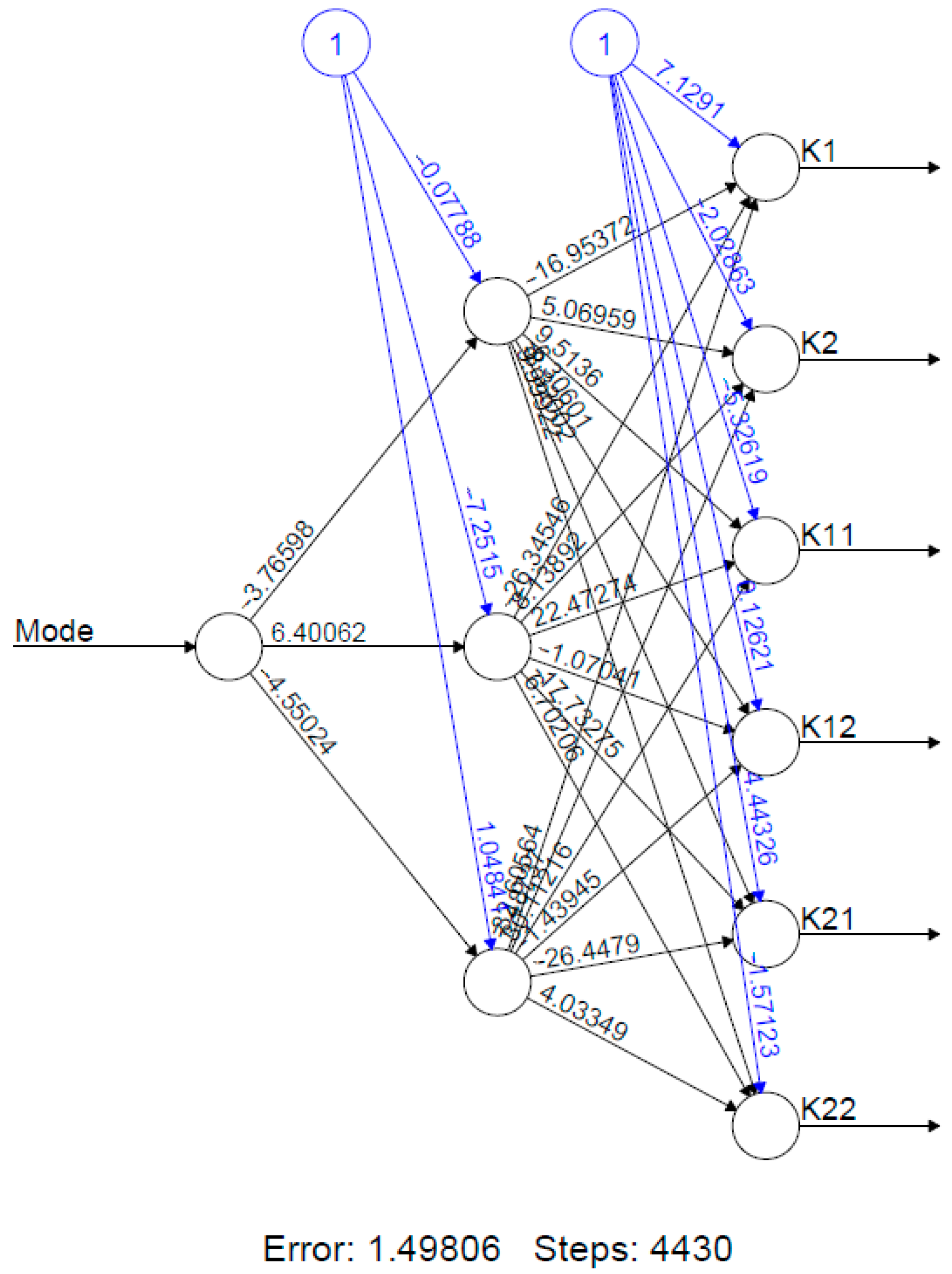
The proposed neural network model based on the SIMO-approximator (see Figure 7) has the structure (1-3-6), i.e., one input, three neurons in the hidden layer with tanh(.) activation function, and six linear outputs, where input “Mode” = (0.68, …, 0.95). Approximation accuracy at the given points is defined by an error equal to 0.003221.
The architecture of the SIMO-approximator is determined by the requirements for the accuracy of solving the approximation problem and has the form:
The results of numerical modeling showed the correspondence of the quality of transient processes to those specified in the formulation of the problem (Figure 8).
6. GTE Lifecycle and Nonlinear Control Design
The criterion for the effectiveness of fatigue tests of a gas turbine engine is traditionally the equality of damage to aircraft engine elements in the operational and test cycles. The fatigue test parameters are selected taking into account one or several main operational cycles. Typical test cycle performs the load of critical engine elements during an operational cycle. The test cycle consists of the consequence of regimes, e.g., engine starting, maximal takeoff, climbing, cruise, descent, etc. The duration of each regime may differ depending on the thermal load of the engine elements. To decrease the test duration, the lower stress regimes might be substituted with higher stress regimes and additional acceleration and deceleration during transient regimes. Thus, it may provoke the engine reaching the stability limit. In this case, design of a nonlinear stable controller for fatigue tests is one of the important tasks.
The lifecycle of a gas turbine engine control system, like any complex technical object, includes predesign stage, design stage, stages of implementation, operation, and disposal [42]. At the predesign stage, the architecture of the control system is formed; in our case, at the design stage, a prototype of the system is developed and tested; at the operational stage, the control system fulfills its purpose. Disposal is the final stage in the lifecycle of a gas turbine engine when it can no longer be used or repaired.
At all stages of the lifecycle of the control system, a sufficiently large amount of information about the characteristics of the control system is generated and collected, which allows us to make the system improvements taking into account this information [43,44]. At the disposal stage, all information about this class of control system can be used in the development of its modification [45].
One of the main reasons for the limited possibilities of building a simulation model of the engine lifecycle for choosing the parameters for testing the controller is the complexity of evaluating the criterion of the effectiveness of testing the controller within the engine lifecycle.
The reason for the emergence of problems of this kind is, first of all, the need for preliminary processing of large volumes of heterogeneous data collected at different stages of the lifecycle of the engine.
Under these conditions, Big Data technology can serve as an effective tool for storing and analyzing controller lifecycle information. For example, Hadoop efficiently manages distributed resources based on access to streaming data. MapReduce allows batch processing of database queries, which dramatically reduces processing time. These technologies are suitable for preprocessing the original model data and the simulation results.
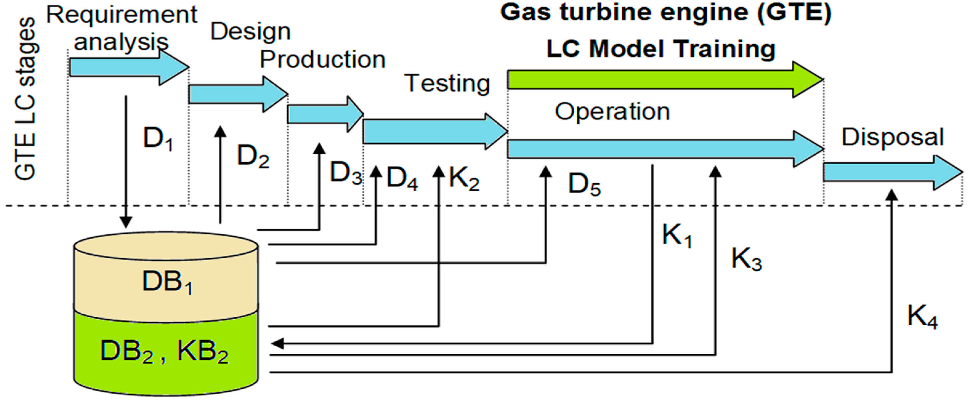
The main data and knowledge flows in lifecycle modeling and controller parameters evaluation are shown in Figure 9, where:
- D1 is a formal gas turbine engine and controller description;
- D2, D3, D4, and D5 are data necessary for gas turbine engine and controller design, production, testing, and operation;
- K1 is the gas turbine engine and controller operation knowledge;
- K2 is control of test parameters;
- K3 is control of operation parameters;
- K4 is disposal control;
- DB1 and DB2 are integrated databases;
- KB2 is knowledge base.
Thus, the information obtained at the testing stage can be used to optimize the performance of the nonlinear controller. However, the design stage of a nonlinear controller presented above is a rather important stage, since it allows for developing a prototype, taking into account the constraints, which ensure the optimization of costs for the development of the entire control system.
7. Conclusions
Gas turbine engines belong to the class of complex heat machines, which are widely used to solve various tasks. Due to their design and functional features, gas turbine engines are nonlinear control objects. The dynamic properties of the gas turbine engine change depending on operating conditions and environmental conditions. As it is known, the characteristics of instances of the same type of engine may also change significantly.
This paper discusses the algorithmic approach for the design of nonlinear control systems for dynamic control objects given by piecewise linear models.
To ensure the required performance indicators in the entire range of operating parameters, it is necessary to meet the requirements for the quality of transient processes when changing the operating regimes of a gas turbine engine.
The design method is based on the assumption that the matrix of the canonical basis of the closed-loop system is constant, which makes it possible to provide the desired performance of control process in the regimes of partial acceleration. This approach allows the use of various methods for the design of linear controllers under the additional condition that the matrix of the canonical basis of the closed-loop system is constant. An example of design for a twin-shaft gas turbine engine is considered.
The design method considered can be used for various types of gas turbine engines. The proposed design method provides the required quality of transient processes in acceleration regimes.
The important component of the effective design of control systems is the collection of possible data about the control object throughout its entire lifecycle. It also allows for continuous improvement of the existing control system and the development of its new modifications.
Achievements in the field of machine learning algorithms, taking into account the above, make it possible to adjust the parameters of nonlinear controllers for a specific instance of the gas turbine engine. However, at the preliminary stage of designing the control system, it is necessary to solve the problems of designing the control system by using available analytical tools and models.
As part of further research, it is planned to take into account the influence of changes in the characteristics of the model under the influence of various noises and possible deviations of its parameters for various instances of the control object.
Author Contributions
Conceptualization, S.V. and N.K.; methodology, S.V.; validation and software, N.K.; supervision: S.V. All authors have read and agreed to the published version of the manuscript.
Funding
This research received no external funding.
Institutional Review Board Statement
Not applicable.
Informed Consent Statement
Not applicable.
Conflicts of Interest
The authors declare no conflict of interest.
Nomenclature
| N1 | Low pressure compressor rotational speed |
| N2 | High pressure compressor rotational speed |
| Wf | Fuel consumption |
| A8 | Jet nozzle cross-sectional area |
| P1 | Compressor average pressure ratio |
| P2 | Inlet corrected mass flow rate |
| R1 | Compressor surge region |
| R2 | Turbine gas temperature limit region |
| R3 | Flameout region |
| L | Steady running line |
| mi | Points on engine steady running line L |
| m1–m4 | Trajectory during acceleration |
| m4–m1 | Trajectory during deceleration |
| B1–B4 | Boundaries of stable operation of the compressor |
| Values of the vectors of variables x, u, y at static (steady-state) operating regimes of a gas turbine engine (i = 1, …, 4) | |
| Vector of state variables (which are understood as the rotational speeds of the low and high pressure compressors of the gas turbine engine, respectively) | |
| Vector of control actions (fuel consumption and jet nozzle cross-sectional area) | |
| Vector of controlled variables (air pressure behind the compressor, gas pressure and temperature behind the turbine) | |
| Parameter that determines the choice of the point of the i-th operating mode (or, respectively, the i-th piecewise linear model) | |
| Relative (dimensionless) values of variables N1 and N2 | |
| λ | Eigenvalue |
| Λ | Spectrum {λ} |
| M | Matrix of eigenvectors |
| t | Time (sec) |
| m | Eigenvector |
| G(.) | Eigenvalue function |
| f(.) | Neural network activation function |
| K | Nonlinear control |
| W | Weight matrix of neural network |
| Abbreviations | |
| SIMO | Single input–multiple output |
| GTE | Gas turbine engine |
References
- Soares, C. Gas Turbines: A Handbook of Air, Land and Sea Applications; Elsevier: Amsterdam, The Netherlands, 2015; pp. 173–254. [Google Scholar]
- MacIsaac, B.; Langton, R. Gas Turbine Propulsion Systems; John Wiley & Sons: New York, NY, USA, 2011; p. 328. [Google Scholar]
- Farokhi, S. Aircraft Propulsion; John Wiley & Sons: New York, NY, USA, 2014; p. 1048. [Google Scholar]
- Mattingly Jack, D. Elements of Propulsion: Gas Turbines and Rockets; AIAA Inc.: Reston, VA, USA, 2006; p. 928. [Google Scholar]
- Jaw, L.C.; Mattingly, J.D. Aircraft Engine Control Design, System Analysis, and Health Monitoring; AIAA Inc.: Reston, VA, USA, 2009. [Google Scholar]
- Gurevich, O.S. Aviation GTE Automatic Control Systems: Encyclopedic Reference; Gurevich, O.S., Ed.; Torus Press: Moscow, Russia, 2011. [Google Scholar]
- Jianguo, S.; Vasilyev, V.; Ilyasov, B. Advanced Multivariable Control Systems of Aeroengines; Sun, J., Vasilyev, V., Ilyasov, B., Eds.; BUAA Press: Beijing, China, 2005. [Google Scholar]
- Yamagami, J.; Okajima, K.; Koyama, O.; Yamamoto, S. Development of next generation gas turbine control systems. IHI Eng. Rev. 2008, 41, 74–79. [Google Scholar]
- Eres, M.H.; Scanlan, J.P. A Hierarchical Life Cycle Cost Model for a Set of Aero-Engine Components. In Proceedings of the 7th AIAA Aviation Technology, Integration and Operations Conference (ATIO), Belfast, Northern Ireland, 18–20 September 2007; AIAA Inc.: Reston, VA, USA, 2007. AIAA 2007-7705. [Google Scholar]
- Schobeiri, M.T. Gas Turbine Design, Components and System Design Integration; Springer: Cham, Switzerland, 2018; pp. 31–47. [Google Scholar]
- Vasilyev, V.; Valeyev, S. Sun Jianguo, Identification of Complex Technical Objects on the Basis of Neural Network Models and Entropy Approach. In Proceedings of the 9th World Multi-Conference on Systemics, Cybernetics and Informatics, Orlando, FL, USA, 10–13 July 2005; Volume IX, pp. 89–93. [Google Scholar]
- Ilyasov, B.; Vasilyev, V.; Valeev, S. Design of Multi-Level Intelligent Control Systems for Complex Technical Objects on the Basis of Theoretical-Information Approach. Acta Polytech. Hung. 2020, 17, 137–150. [Google Scholar] [CrossRef]
- Kulikov, G.G.; Thompson, H.A. Dynamic Modelling of Gas Turbines: Identification, Simulation, Condition Monitoring and Optimal Control, Advances in Industrial Control; Springer: London, UK, 2014. [Google Scholar]
- Kulikov, G.G.; Arkov, V.Y.; Abdulnagimov, A.I. Markov modelling for energy efficient control of gas turbine power plant. IFAC Proc. Vol. 2010, 43 Pt 1, 63–67. [Google Scholar] [CrossRef]
- Leith, D.J.; Leithead, W.E. Gain-scheduled and nonlinear systems: Dynamics analysis by velocity based linearization families. Int. J. Control 1998, 70, 289–317. [Google Scholar] [CrossRef]
- Pakmehr, M.; Fitzgerald, N.; Feron, E.M.; Shamma, J.S.; Behbahani, A. Gain Scheduling Control of Gas Turbine Engines: Stability by Computing a Single Quadratic Lyapunov Function. In Proceedings of the ASME Turbo Expo 2013: Turbine Technical Conference and Exposition, San Antonio, TX, USA, 3–7 June 2013. GT2013-96012, V004T06A027. [Google Scholar]
- Shamma, J.S.; Athans, M. Analysis of Gain Scheduled Control for Nonlinear Plants. IEEE Trans. Autom. Control 1990, 35, 898–907. [Google Scholar] [CrossRef]
- Sisworahardjo, N.; El-Sharkh, M.; Alam, M. Neural network controller for microturbine power plants. Electr. Power Syst. Res. 2008, 78, 1378–1384. [Google Scholar] [CrossRef]
- Nise, N.S. Control Systems Engineering; John Wiley & Sons: New York, NY, USA, 2019. [Google Scholar]
- Friedland, B. Control System Design: An Introduction to State-Space Methods; Dover: New York, NY, USA, 2005. [Google Scholar]
- Katsuhiko, O. Modern Control Engineering; Prentice Hall: Upper Saddle River, NJ, USA, 2010. [Google Scholar]
- Kolesnikov, A.A.; Kolesnikova, S.I. Synthesis Algorithm for a Continuous Robust Regulator on a Manifold for a Manipulator under Non-Random Noise Conditions. In Proceedings of the 2020 International Russian Automation Conference (RusAutoCon 2020), Sochi, Russia, 6–12 September 2020; pp. 291–295. [Google Scholar]
- Akhmetgaleev, I.I. Design of Nonlinear Control Systems with Matrix Approach; St. Petersburg State University of Aerospace Instrumentation Publ.: St. Petersburg, Russia, 1983. [Google Scholar]
- Akhmetgaleev, I.I. Design of Nonlinear Control Systems; St. Petersburg State University of Aerospace Instrumentation Publ.: St. Petersburg, Russia, 1984. [Google Scholar]
- Cybenko, G. Approximation by superpositions of a sigmoidal function. Math. Control Signals Syst. 1989, 2, 303–314. [Google Scholar] [CrossRef]
- Hornik, K.M.; Stinchombe, M.; White, H. Multilayer feedforward networks are universal approximators. Neural Netw. 1989, 2, 359–366. [Google Scholar] [CrossRef]
- Funahashi, K. On the approximate realization of continuous mappings by neural networks. Neural Netw. 1989, 2, 183–192. [Google Scholar] [CrossRef]
- Pinkus, A. Approximation theory of the MLP model in neural networks. Acta Numer. 1999, 8, 143–195. [Google Scholar] [CrossRef]
- Gorban, A.N. Approximation of continuous functions of several variables by an arbitrary nonlinear continuous function of one variable, linear functions, and their superpositions. Appl. Math. Lett. 1998, 11, 45–49. [Google Scholar] [CrossRef] [Green Version]
- Vasilyev, V.; Ilyasov, B.; Kusimov, S. Neurocomputers in Aviation; Radiotechnica Pub.: Moscow, Russia, 2004. [Google Scholar]
- Valeev, S.; Kondratyeva, N. Design of Nonlinear Multi-Mode Controller for Gas Turbine Engine in State Space Based on Algorithmic Approach. In Proceedings of the 2020 International Russian Automation Conference (RusAutoCon 2020), Sochi, Russia, 6–12 September 2020; pp. 1053–1057. [Google Scholar]
- Sanchez, E.N.; Rios, J.D.; Alanis, A.Y.; Arana-Daniel, N. Neural Networks Modeling and Control; Academic Press: Cambridge, MA, USA, 2020. [Google Scholar]
- Agarwal, M. A systematic classification of neural-network-based control. Control Syst. 1997, 17, 75–93. [Google Scholar]
- Narendra, K.S.; Mukhopadhyay, S. Adaptive control using neural networks and approximate models. IEEE Trans. Neural Netw. 1997, 8, 475–485. [Google Scholar] [CrossRef] [PubMed]
- Mu, J.; Rees, D.D. Approximate model predictive control for gas turbine engines. In Proceedings of the 2004 American Control Conference, Boston, MA, USA, 30 June–2 July 2004; Volume 1/6, pp. 5704–5709. [Google Scholar]
- Sahin, S.; Savran, A. A neural network approach to model predictive control. In Proceedings of the 14th Turkish Symposium on Artificial Intelligence and Neural Networks, Izmir, Turkey, 16–17 June 2005; pp. 386–392. [Google Scholar]
- Galushkin, A.I. Neural, Networks Theory; Springer: Cham, Switzerland, 2007. [Google Scholar]
- Wonham, W.M. Linear Multivariable Control: A Geometric Approach; Springer: Cham, Switzerland, 1985. [Google Scholar]
- Park, H.; Seborg, D.E. Eigenvalue Assignment Using Proportional-Integral Feedback Control. Int. J. Control 1974, 20, 517–523. [Google Scholar] [CrossRef]
- The R Project for Statistical Computing. Available online: https://www.r-project.org/ (accessed on 20 December 2020).
- GNU Octave. Available online: http://www.gnu.org/software/octave/ (accessed on 21 December 2020).
- Guichvarov, A.; Kondratieva, N. Technical and economic assessment of aircraft engines fatigue testing on base of simulation modeling. In Proceedings of the 37th AIAA/ASME/SAE/ASEE Joint Propulsion Conference and Exhibit, Salt Lake City, UT, USA, 8–11 July 2001; AIAA Inc.: Reston, VA, USA, 2007. [Google Scholar]
- Kondratyeva, N.; Valeev, S. Fatigue Test Optimization for Complex Technical System on The Basis of Lifecycle Modeling and Big Data Concept. In Proceedings of the 2016 IEEE 10th Int. Conf. on Application of Information and Communication Technologies, Baku, Azerbaijan, 12–14 October 2016; IEEE Publishing: New York, NY, USA, 2016; pp. 1–4. [Google Scholar]
- Zagitova, A.; Kondratyeva, N.; Valeev, S. Information Support of Gas-Turbine Engine Life Cycle Based on Agent-Oriented Technology. In Proceedings of the 5th Int. Conf. on Industrial Engineering (ICIE 2019), Sochi, Russia, 25–29 March 2019; Radionov, A.A., Kravchenko, O.A., Guzeev, V.I., Rozhdestvenskiy, Y.V., Eds.; Springer: Cham, Switzerland, 2020; Volume I, pp. 469–476. [Google Scholar]
- GT Auto Tuner: First System Worldwide to Leverage Physics and Reinforcement Learning to Optimize Gas Turbine Operation. Available online: https://www.siemens-energy.com/global/en/offerings/services/digital-services/gt-autotuner.html (accessed on 17 December 2020).
Figure 1.
Simplified structural diagram of a gas turbine engine as a control object.

Figure 2.
Typical compressor performance map.

Figure 3.
Architecture of the single input multiple output neural network (single input–multiple output (SIMO)-approximator).
Figure 3.
Architecture of the single input multiple output neural network (single input–multiple output (SIMO)-approximator).

Figure 4.
Diagram of the nonlinear control design algorithm for the gas turbine engine (GTE).

Figure 5.
Nonlinear control system of the gas turbine engine (GTE).

Figure 6.
SIMO-neural network approximator of the coefficients of the dynamic model (20).

Figure 7.
Nonlinear controller based on the SIMO-approximator.

Figure 8.
Transient processes curves for the given regime (the blue line represents the given process and the green line represents the simulation results).
Figure 8.
Transient processes curves for the given regime (the blue line represents the given process and the green line represents the simulation results).

Figure 9.
Data and knowledge flows in gas turbine engine lifecycle modeling.


Table 1.
The values of the parameters of the dynamic model of the gas turbine engine [13].
Table 1.
The values of the parameters of the dynamic model of the gas turbine engine [13].
| No. | Vector of the Model Coefficients | ||||
|---|---|---|---|---|---|
| 0.68 (m.1) | 0.78 (m.2) | 0.89 (m.3) | 0.95 (m.4) | ||
| 1 | a11 | −2.14 | −2.53 | −6.24 | −5.89 |
| 2 | a12 | 1.6 | 1.49 | 1.62 | 1.22 |
| 3 | a21 | −0.11 | −0.37 | −0.53 | −0.55 |
| 4 | a22 | −1.14 | −1.17 | −1.16 | −1.16 |
| 5 | b11 | 3.21 | 2.45 | 2.81 | 2.54 |
| … | … | … | … | … | … |
| 25 | p2st | 0.7 | 0.8 | 0.9 | 1 |
| 26 | p4st | 0.14 | 0.19 | 0.24 | 0.31 |
| 27 | T4st | 0.09 | 0.13 | 0.19 | 0.24 |
Publisher’s Note: MDPI stays neutral with regard to jurisdictional claims in published maps and institutional affiliations. |
© 2021 by the authors. Licensee MDPI, Basel, Switzerland. This article is an open access article distributed under the terms and conditions of the Creative Commons Attribution (CC BY) license (http://creativecommons.org/licenses/by/4.0/).
Share and Cite
MDPI and ACS Style
Valeev, S.; Kondratyeva, N. Design of Nonlinear Control of Gas Turbine Engine Based on Constant Eigenvectors. Machines 2021, 9, 49. https://0-doi-org.brum.beds.ac.uk/10.3390/machines9030049
AMA Style
Valeev S, Kondratyeva N. Design of Nonlinear Control of Gas Turbine Engine Based on Constant Eigenvectors. Machines. 2021; 9(3):49. https://0-doi-org.brum.beds.ac.uk/10.3390/machines9030049
Chicago/Turabian StyleValeev, Sagit, and Natalya Kondratyeva. 2021. "Design of Nonlinear Control of Gas Turbine Engine Based on Constant Eigenvectors" Machines 9, no. 3: 49. https://0-doi-org.brum.beds.ac.uk/10.3390/machines9030049
Note that from the first issue of 2016, this journal uses article numbers instead of page numbers. See further details here.