Article

Precision Interaction Force Control of an Underactuated Hydraulic Stance Leg Exoskeleton Considering the Constraint from the Wearer

1
School of Mechanical Engineering, Hefei University of Technology, Hefei 230009, China
2
Anhui Engineering Laboratory of Intelligent CNC Technology and Equipment, Hefei 230009, China
*
Author to whom correspondence should be addressed.
Submission received: 31 March 2021 / Revised: 5 May 2021 / Accepted: 6 May 2021 / Published: 10 May 2021
(This article belongs to the Special Issue Advanced Control of Industrial Electro-Hydraulic Systems)

Abstract

:
Hydraulic lower limb exoskeletons are wearable robotic systems, which can help people carry heavy loads. Recently, underactuated exoskeletons with some passive joints have been developed in large numbers for the purpose of decreasing the weight and energy consumption of the system. There are many control algorithms for a multi-joint fully actuated exoskeleton, which cannot be applied for underactuated systems due to the reduction in the number of control inputs. Besides, since the hydraulic actuator is not a desired force output source, there exist high order nonlinearities in hydraulic exoskeletons, which makes the controller design more challenging than motor driven exoskeleton systems. This paper proposed a precision interaction force controller for a 3DOF underactuated hydraulic stance leg exoskeleton. First, the control effect of the wearer is considered and the posture of the exoskeleton back is assumed as a desired trajectory under the control of the wearer. Under this assumption, the system dynamics are changed from a 3DOF underactuated system in joint space to a 2DOF fully actuated system in Cartesian space. Then, a three-level interaction force controller is designed in which the high-level controller conducts human motion intent inference, the middle level controller tracks human motion and the low-level controller achieves output force tracking of hydraulic cylinders. The MIMO adaptive robust control algorithm is applied in the controller design to effectively address the high order nonlinearities of the hydraulic system, multi-joint couplings and various model uncertainties. A gain tuning method is also provided to facilitate the controller gains selection for engineers. Comparative simulations are conducted, which demonstrate that the principal human-machine interaction force components can be minimized and good robust performance to load change and modeling errors can be achieved.

1. Introduction

Devices that can augment human performance in heavy load carrying applications have attracted great interest from researchers in recent decades. Many solutions have been proposed, such as back support exoskeletons [1], upper limb exoskeletons [2,3,4] and lower limb exoskeletons [5]. A lower limb exoskeleton that augments the human performance is a human-machine integrated system in which the wearer has functions of navigation, balance, and coordinate control, while the robot is used to carry heavy load and follow human motion. It combines human intelligence with robot power and has wide applications in soldier marching, earthquake rescue and construction sites [6,7,8]. Due to the high power-to-weight ratio, hydraulic actuators are widely used in the development of such systems which need to be a small size while providing a large force. In recent years, many underactuated lower limb exoskeleton systems with some passive joints have been proposed so that the weight and system energy consumption can be decreased [9,10,11,12,13]. In these systems, the ankle joint is usually passive due to the small power requirements in human walking. As for the hip and knee joints, the actuation condition is different in different prototypes.
Different from exoskeletons or robots for rehabilitation, in which a predefined or desired gait trajectories are known in advance [14,15,16], human motion trajectory of the healthy wearer cannot be known in advance in an exoskeleton for human performance augmentation. Due to the heavy loads and large actuation forces, the wearer will also not be able to move or bear a large force from the heavy load if the control algorithm is not well designed. Thus, there is a higher requirement on dynamic modeling and controller design for exoskeleton systems which augment human performance. The control goal of lower limb exoskeleton for human performance augmentation minimizes the human–machine interaction force so that human motion can be tracked accurately by the exoskeleton and little load force can be felt by the wearer. However, with less control input, strong coupled high-order nonlinearities of hydraulic system, various parameter uncertainties and modeling errors bring tremendous difficulties to the control algorithm design for underactuated hydraulic lower limb exoskeleton.
To deal with strong coupled high-order nonlinearities, various parameter uncertainties and modeling errors, many robust control methods have been proposed to minimize the human–machine interaction force. In [17], a probabilistic sensitivity amplification control method is proposed to achieve good disturbance rejection and robust performance to parameter variation. In [18], a nonlinear disturbance observer was integrated into the conventional proxy-based sliding mode control structure to enhance the robust performance to model uncertainties. Using a disturbance observer, an impedance control structure has been proposed in [19]. In order to improve the performance of the impedance controller, the controller parameter optimization method and human–robot interaction dynamics modeling using some AI algorithms are also proposed [20,21]. Adaptive control algorithms are also often used in the controller design, such as adaptive assist-as-needed control [22] and adaptive sliding mode control [23]. Combining the advantages of adaptive control with that of robust control, an adaptive robust control (ARC) algorithm has been developed for high speed and high precision control of uncertain nonlinear systems [24,25], which is also adopted to the robust interaction force control of hydraulic lower limb exoskeletons [26,27]. However, all these interaction force control methods are proposed for fully actuated systems. Due to the reduction in the number of control inputs, these fully actuated control methods cannot be directly applied for those underactuated ones.
As for controller design of underactuated exoskeleton, some works have been carried out. One method simply neglects the passive joint and only considers the actively actuated joint in the dynamic modeling. In [28,29], a sliding mode control algorithm as well as an admittance controller were developed for a three-joints swing leg exoskeleton based on a 2DOF dynamic model with only hip and knee joints. Another method is to neglect the multi-joint coupling and control the active joint independently, such as the finite-state assistive control in [30] and a hybrid control strategy in [31]. In [32], the sliding mode controller is designed for the swing leg assuming that all the joints are actuated and, finally, the computed control input for an actual actively actuated joint is used for an underactuated exoskeleton. As for the stance leg, a PD control algorithm was proposed. In [12], the two legs are controlled separately. A model-free adaptive human–robot interaction minimization control strategy is proposed for swing leg while a static balance control algorithm is proposed for stance leg. Due to neglecting the dynamic modeling of the whole system, the theoretic analysis of control performance is not given in the paper. In general, these existing controllers for an underactuated exoskeleton only involve preliminary control in which a simplified controller algorithm or system dynamic model is used. As for the existing stance leg control in underactuated exoskeleton, most control methods are based on PID control. Considering the reduction in the number of control inputs, strong coupled high-order nonlinearities of hydraulic system and various model uncertainties, it is still a challenging issue for high accuracy force control for an underactuated hydraulic exoskeleton.
In [33], a complete dynamic modeling considering the control effect of the wearer is conducted and a two-level adaptive robust force controller is designed for motor driven underactuated single leg exoskeleton system. In this study, the problem is extended to the high-performance interaction force control for underactuated exoskeleton driven by hydraulic cylinders, which brings more challenging issues. Compared to a motor, a hydraulic actuator is not a desired force output source, the dynamics of a hydraulic exoskeleton system is at least three ordered from the control voltage of valves to the joint position while it is usually two ordered for motor driven exoskeleton. Also, there exist large numbers of parameter uncertainties and modeling errors in hydraulic system [34,35]. The high order nonlinearities and various model uncertainties of a hydraulic system makes it more challenged to control the underactuated exoskeleton driven by hydraulic actuators.
In order to address the problem of lacking control inputs, we consider the control effect of the wearer. The posture of the exoskeleton’s back is assumed as a desired trajectory under the control of the wearer. With this holonomic constraint from the wearer, the system dynamics is changed from a 3DOF underactuated system in joint space to a 2DOF fully actuated system in Cartesian space. A three-level interaction force controller is designed in which the high-level controller conducting human motion intent inference, the middle level controller tracking human motion and the low-level controller achieving output force tracking of hydraulic cylinders. The MIMO Adaptive robust control algorithm is applied in the controller design to effectively address the high order nonlinearities of the hydraulic system, various parameter uncertainties and modeling errors. A gain tuning method is also given to facilitate the controller gains selection for engineers. Comparative simulation results verify that the principal interaction force components can be minimized and good robust performance to load change, variation of exoskeleton back posture and human machine interface modeling errors can be achieved.
The principal contributions of this paper are as follows:
(1)
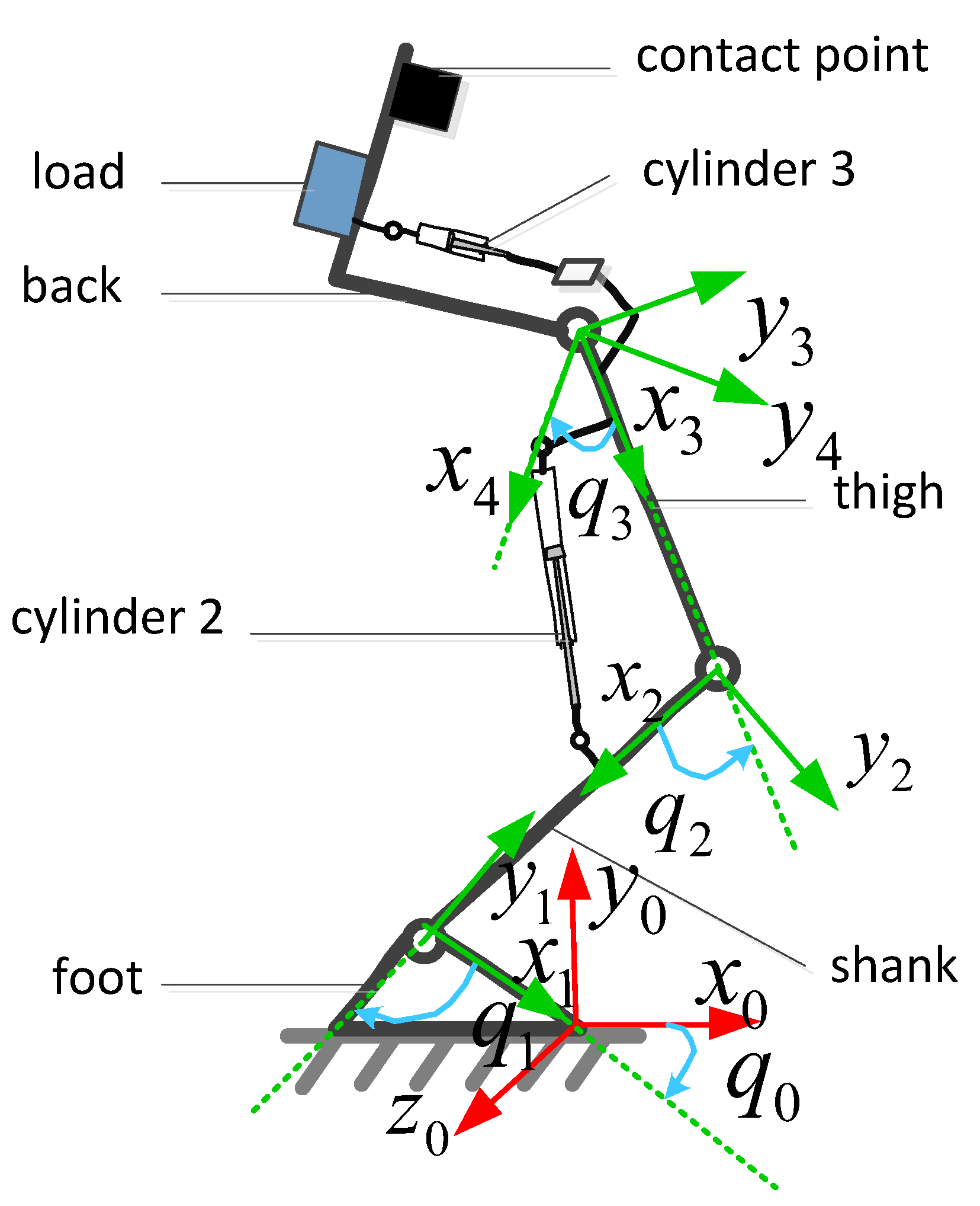
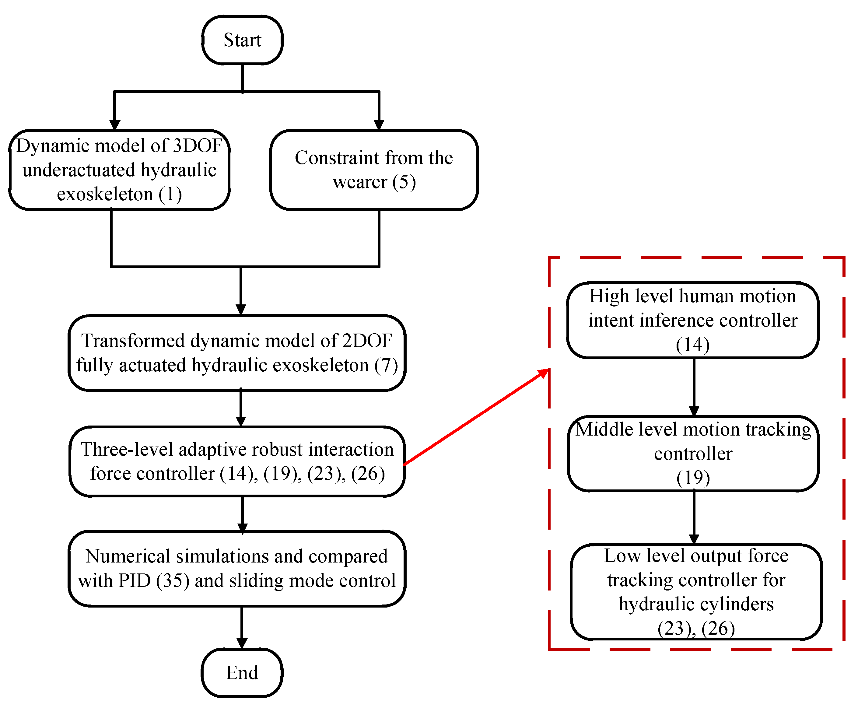
Considering the control effect of the wearer, a holonomic constraint from the wearer is added to system dynamics, which help transform the dynamics of a 3DOF underactuated exoskeleton in joint space into a 2-DOF fully actuated system in Cartesian space. Parameter uncertainties (such as stiffness of human machine interface, parameters of hydraulic actuator and load changes) and uncertain nonlinearities (such as external disturbance and unmodeled dynamics) are considered in the modeling.
(2)
A three level adaptive robust controller is proposed for an underactuated hydraulic stance exoskeleton to effectively deal with strong coupled high-order nonlinearities of a hydraulic system, various parameter uncertainties and modeling errors and precise interaction force control under various parameter uncertainties and uncertain nonlinearities is achieved.

2. System Dynamics

2.1. Dynamic Model

Figure 1 shows the schematic diagram of a 3DOF underactuated hydraulic stance leg exoskeleton, which includes a passive ankle joint, a hydraulic cylinder actuated hip joint and a hydraulic cylinder actuated knee joint. In this paper, we only consider walking on a flat terrain. Since human dynamics modeling is very complicated (including the skeletal-muscles model, human motion controller, etc.), it is difficult to model the human accurately. Considering the controller design, in our modeling, we do not establish the human model. The wearer is regarded to provide a desired motion trajectory. Then, a human machine interface dynamic model is established to describe the relationship between human–machine interaction force and the motion tracking error between human and exoskeleton. Thus, the dynamics of a single leg exoskeleton contains three parts: human machine interface dynamics, the mechanical structure dynamics and the hydraulic actuator dynamics. Considering only the main compliant properties in human machine interface modeling, a spring model with unknown stiffness is used to describe the main compliant property of the interface. As for other unmodeled uncertainties, we consider them in the lumped model uncertainties. In the later part, an adaptive robust controller is designed to deal with the model uncertainties in the human/robot attachment model. The system dynamic equations are given as:
d d t 0 t F hm d τ = K x h x e + D ˜ 1 q = i n v k i n e ( x e ) 0 τ act + J T q F hm = M sp 3 q q ¨ + C sp 3 q , q ˙ q ˙ + G sp 3 q + B q ˙ + D ˜ 2 τ act = τ 2 , τ 3 T τ i = ( P 1 i A 1 i P 2 i A 2 i ) x L i q i V 1 i β e P ˙ 1 i = A 1 i x L i q i q ˙ i + Q 1 i + D ˜ 31 i V 2 i β e P ˙ 2 i = A 2 i x L i q i q ˙ i + Q 2 i + D ˜ 32 i Q 1 i = k q 1 i x v i Δ P 1 i , Q 2 i = k q 2 i x v i Δ P 2 i Δ P 1 i = P s P 1 i i f x v i 0 P 1 i P r i f x v i < 0 Δ P 2 i = P 2 i P r i f x v i 0 P s P 2 i i f x v i < 0 x v i = u i , i = 2 , 3 ,
where F hm = F h m x F h m y τ e z T is the human-machine interaction force vector at back. K = d i a g { K x , K y , K z } is the stiffness of human–machine interface. x h = x h x x h y x h z T is the human position at the back. x e = x e x x e y x e z T is the exoskeleton position at the back. q = q 1 q 2 q 3 , T is the joint position. q can be computed from x e through inverse kinematics, that is q = i n v k i n e ( x e ) . τ act = τ 2 , τ 3 T is the joint torque at knee and hip joint. J = x e q is the Jacobian matrix. M sp 3 ( q ) is the inertial matrix. C sp 3 ( q , q ˙ ) q ˙ is centrifugal/Coriolis force. G sp 3 ( q ) is gravity force. B = d i a g { B 1 , B 2 , B 3 } is damping ratio in the system. Since it is hard to obtain an accurate friction model, in the paper we just consider the linear friction force at the joints. The unmodeled errors of friction force can be considered as lumped disturbances and will be attenuated through the proposed robust control. x L i is the position of the cylinder i. x L i q i is the partial derivative of x L i to q i . P 1 i and P 2 i are pressures of both chambers in cylinder i. A 1 i and A 2 i are areas of the both chambers in cylinder i. V 1 i = V h 1 i + A 1 i x L i and V 2 i = V h 2 i + A 2 i x L i are volumes of both chambers in cylinder i. V h 1 i , V h 2 i are two chamber volumes when q i = 0 . β e represents the effective bulk modulus. Q 1 i , Q 2 i are flows of both chamber in cylinder i. k q 1 i and k q 2 i represent the flow gain coefficients of cylinder i chambers. x v i represents the displacement of valve i. P s represents the supply pressure. P r is tank pressure. D ˜ 1 , D ˜ 2 , D ˜ 31 i and D ˜ 32 i are lumped disturbances. Since
x ˙ e = J q ˙ , x ¨ e = J ˙ q ˙ + J q ¨ ,
thus, the mechanical structure dynamics described in joint space can be transformed into Cartesian space which has the following form
J T 0 τ act + F hm = M x x ¨ e + C x x ˙ e + G x + B x x ˙ e + J T D ˜ 2 ,
where
M x = J T M sp 3 J 1 C x = J T C sp 3 J 1 J T M sp 3 J 1 J ˙ J 1 G x = J T G sp 3 , B x = J T B J 1 .
In a 3DOF underactuated exoskeleton system, there exist three independent joints but with only two hydraulic cylinders. Thus, there is one interaction force which is unable to be minimized by the hydraulic cylinders. Usually, for underactuated manipulator, there exist uncontrolled internal dynamics due to lacking control input [36,37]. However, as a human robot integrated system, the wearer participates in the control of the exoskeleton as well. As we know, the human brain is an excellent controller and there also exist various actuators and sensors in the human body. Thus, we can assume that the wearer can keep the balance of the exoskeleton and a torque ( τ e z ) can be provided by the wearer to make the exoskeleton back posture ( x e z ) be a desired trajectory. Based on this assumption, a holonomic constraint equation can be obtained
x e z = x e z d t ,
where x e z d is a desired trajectory. We can get the following equations by differentiating (5) while noting (3),
J T 0 τ act + F h m x F h m y τ e z = M x x ¨ e + C x x ˙ e + G x + B x x ˙ e + J T D ˜ 2 x ¨ e z = x ¨ e z d t .
Here, we have 4 unknown variables ( x ¨ e , τ ez ) and 4 equations Equation (6). Regarding τ act , F hmx and F hmy as inputs, we can compute x ¨ e and τ ez as follows:
x ¨ e z = x ¨ e z d ( t ) x ¨ ea = M ea 1 ( B ea τ act C ea x ˙ ea G ea B xea x ˙ ea u 1 J T D ˜ 2 u 1 C nst ) τ ez = M ea 2 x ¨ ea + C ea 2 x ˙ ea + G ea 2 + B xea 2 x ˙ ea + B ea 2 τ act + u 2 J T D ˜ 2 + u 2 C nst ,
where x ea = x e x x e y T , M ea = u 1 M x u 6 , B ea = u 1 J T u 3 , C ea = u 1 C x u 6 , G ea = u 1 G x , B xea = u 1 B x u 6 , M ea 2 = u 2 M x u 6 , C ea 2 = u 2 C x u 6 , G ea 2 = u 2 G x , B xea 2 = u 2 B x u 6 , B ea 2 = u 2 J T u 3 , C nst = M x u 7 x ¨ ezd ( t ) + C x u 7 x ˙ ezd ( t ) + B x u 7 x ˙ ezd ( t ) u 5 F hmx u 8 F hmy . u 1 = 1 0 0 0 1 0 , u 2 = 0 0 1 , u 3 = 0 0 1 0 0 1 , u 6 = 1 0 0 1 0 0 , u 7 = 0 0 1 , u 8 = 0 1 0 .
The dynamics described in (7) is a fully actuated system in which the second equation has the following properties
Property 1: M ea ( q ) is an s.p.d. matrix.
Property 2: M ˙ ea q 2 C ea q , q ˙ is a skew-symmetric matrix.
Property 3: M ea ( q ) , C ea ( q ) , G ea ( q ) satisfy,
M ea q x ¨ r + C ea q , q ˙ x ˙ r + G ea q = f 0 q , q ˙ , x ˙ r , x ¨ r + Y ( q , q ˙ , x ˙ r , x ¨ r ) β ,
where x ˙ r and x ¨ r are any assignable vectors. β represents the system parameter vector of exoskeleton.

2.2. State Space Equation

The lumped disturbances are defined as:
Δ ˜ 1 a = u 1 ( x h + K 1 D ˜ 1 ) , Δ ˜ 3 a = u 1 J T D ˜ 2 u 1 C nst Δ ˜ 4 a = D ˜ 312 β e A 12 V 12 D ˜ 322 β e A 22 V 22 D ˜ 313 β e A 13 V 13 D ˜ 323 β e A 23 V 23 T Δ ˜ i = Δ i n + Δ i , i = 1 a , 3 a , 4 a ,
where Δ i n is the constant part of Δ ˜ i while Δ i is the time-varying part. Because accurate parameters are impossible to be obtained, a set of system parameters can be defined as:
K θ a = 1 / K x 1 / K y T , Δ 1 an = Δ 1 a n x Δ 1 a n y T B θ = B 1 B 2 B 3 T , Δ 3 an = Δ 3 a n x Δ 3 a n y T Δ 4 an = Δ 4 a n 1 Δ 4 a n 2 T θ F = K θ a T Δ 1 a n T T , θ q = β T B θ T Δ 3 a n T T θ u = β e Δ 4 a n T T .
Assume the parameters and lumped disturbances are bounded. Define the following state variables:
F hmxy = F h m x F h m y T , K xy = d i a g { K x , K y } x 1 a = 0 t F hmxy d τ , x 2 a = x ea , x 3 a = x ˙ ea x 4 a = P 1 = P 12 P 13 T x 5 a = P 2 = P 22 P 23 T x = x 1 a x 2 a x 3 a x 4 a x 5 a T
the state space equations can finally be expressed as:
x ˙ 1 a = K xy x 2 a + K xy Δ 1 an + K xy Δ 1 a x ˙ 2 a = x 3 a x ˙ 3 a = M ea 1 ( B ea τ act C ea x 3 a G ea B xea x 3 a + Δ 3 an + Δ 3 a ) τ act = h F L F ˙ L = Q L β e q v x 3 a β e + Δ 4 an + Δ 4 a Q L = K q u ,
where
h = d i a g x L 2 q 2 , x L 3 q 3 A 1 = d i a g A 12 , A 13 A 2 = d i a g A 22 , A 23 F L = A 1 x 4 A 2 x 5 Q L = Q 12 A 12 V 12 + Q 22 A 22 V 22 Q 13 A 13 V 13 + Q 23 A 23 V 23 T q v 1 = ( A 12 2 V 11 + A 22 2 V 21 ) x L 1 q 1 J 1 q v 2 = ( A 13 2 V 11 + A 23 2 V 21 ) x L 1 q 1 J 1 q v = d i a g q v 1 , q v 2 K q 1 = K q 12 A 12 V 12 Δ P 12 + K q 22 A 22 V 22 Δ P 22 K q 2 = K q 13 A 13 V 13 Δ P 13 + K q 23 A 23 V 23 Δ P 23 K u = d i a g K q 1 , K q 2 .

2.3. Problem Statement

Since the wearer needs to provide a human machine interaction torque around Z axis ( τ e z ) to let the exoskeleton back posture x e z track the desired trajectory ( x e z d ), this interaction torque around Z axis cannot be minimized. However, for the rest two interaction force ( F h m x , F h m y ), we are able to make them small by controlling two hydraulic cylinders. Thus, based on (12), the control goal is to generate a valves control voltage u = u 2 u 3 T to minimizing the integral of interaction force at x and y axis ( x 1 a ).

3. Interaction Force Controller Design

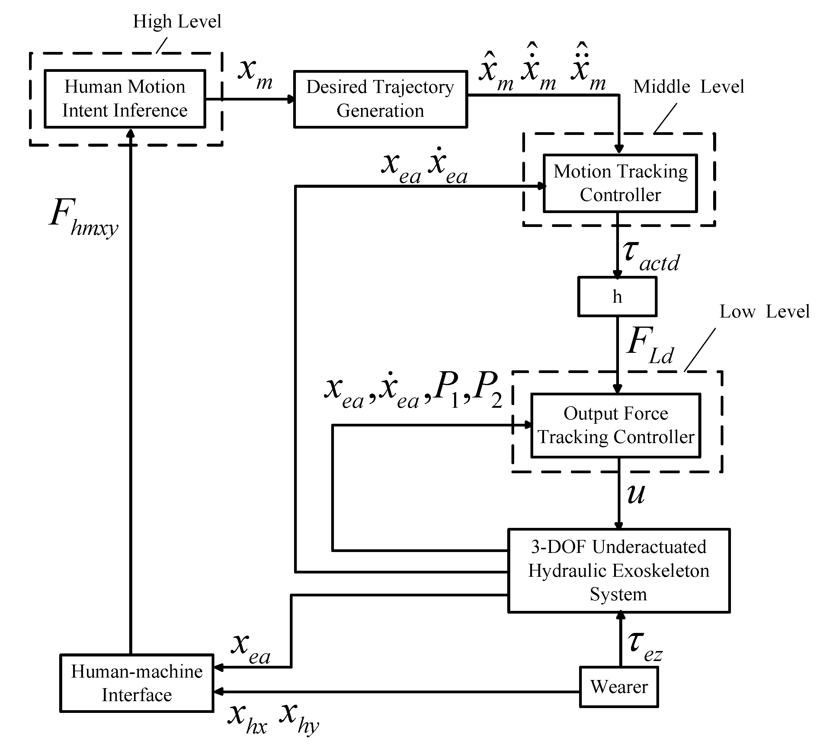
3.1. Overall Control Structure

Different from exoskeletons for rehabilitation, in which a predefined gait trajectory is known in advance, human motion trajectory of the healthy wearer cannot be known in advance in an exoskeleton for human performance augmentation. Thus, control algorithms should be designed to infer the human motion intent and track the human motion trajectory. The proposed interaction force controller includes three levels. The high level is to infer the human motion intent from measured human machine interaction force. Specifically, the exoskeleton position at contact point x 2 a is treated as a virtual control input and a control law x m is designed to make the integral of human–machine force converge to zero. In order to obtain the derivatives of the desired position, an output differential observer is also adopted. The middle controller is to track the desired motion trajectory generated from the high-level controller. Specifically, joint torque τ act is treated as a virtual control input and a control law τ actd is designed to minimize the motion tracking error. The low level is to do output force tracking for hydraulic cylinders so that the hydraulic cylinders can become a desired force output source. Specifically, the control voltage u is designed to minimize the output force tracking error. Adaptive robust control is an effective control algorithm to address both parametric uncertainties and uncertain nonlinearities with a number of successful applications, thus, it is applied in our proposed force controller design. The whole control structure is demonstrated in Figure 2.

3.2. High Level-Human Motion Intent Inference

In this part, the first Equation of (12) is used. The exoskeleton position at contact point x 2 a = x e x x e y T is treated as virtual control input. The control objective is to synthesize a control law x m for x 2 a making the force error z 1 a = x 1 a x 1 ad converges to zero or to be bounded. x m can be described as
x m = x ma + x ms x ma = K ^ f x ˙ 1 ad + Δ ^ 1 an = f θ F ( x 1 ad ) Y θ F ( x 1 ad ) θ ^ F x ms = K 1 z 1 a + x msn θ ^ ˙ F = P r o j ( Γ 1 Y θ F T z 1 a ) P r o j i ( i ) = 0 i f θ ^ F i = θ F max i a n d i > 0 0 i f θ ^ F i = θ F min i a n d i < 0 i o t h e r w i s e ,
where x ma is the adaptive model compensation term, x ms is the robust feedback item. K f = K xy 1 . f θ F and Y θ F are quantities which are known in advance. K 1 = d i a g K 1 x , K 1 y is the gain matrix for linear feedback. Γ 1 > 0 is the matrix for adaptation rate. The nonlinear feedback x msn is required to satisfy:
z 1 a T ( Δ 1 a + 1 2 K ˙ f z 1 a + Y θ F θ ˜ F x msn ) ε 1 z 1 a T x msn 0 ,
where ε 1 > 0 is a design parameter. θ ˜ F = θ ^ F θ F is the error for parameter estimation. Let z 2 h = x 2 a x m . Then the first error dynamics is given as:
K f z ˙ 1 a = K 1 z 1 a z 2 h + Δ 1 a + Y θ F θ ˜ F x msn .
It can be seen that the interaction force becomes 0 or bounded when x 2 a = x m . Thus x m is treated as the inferred human motion intention. In order to obtain the desired position and its derivatives for middle level controller design, similar to [27], an output differential observer is adopted.

3.3. Middle Level-Motion Tracking Controller

In middle level controller design, both second and third dynamic Equation of (12) are used. τ act is treated as control input in this part. The control goal is designing a virtual control law τ actd for τ act minimizing the position tracking error z 2 = x 2 a x ^ m .
First, a quantity z 3 is given as
z 3 = z ˙ 2 + K 2 z 2 = x 3 a x ˙ r , x ˙ r = Δ x ^ ˙ m K 2 z 2 ,
where K 2 is gain matrix for linear feedback. since it is a stable transfer function for G p s = z 2 s / z 3 s = d i a g 1 s + K 2 i , i = 1 , 2 , the following is making z 3 small. Let B xea x 3 a = Y B B θ . the dynamics of z 3 can be obtained by differentiating (17) while paying attention to property 3 and Equation (12):
M ea z ˙ 3 + C ea z 3 = B ea τ act f 0 Y β Y B B θ + Δ 3 an + Δ 3 a ,
the control law τ actd is given as follows:
τ actd = τ acta + τ acts τ actda = B ea 1 ( f 0 + Y β ^ + Y B B ^ θ Δ ^ 3 an ) τ actds = B ea 1 K 3 z 3 + τ actsn ϕ 3 = Y Y B I 2 × 2 T θ ^ ˙ q = P r o j ( Γ 2 ϕ 3 z 3 ) ,
where τ actda is a term for model compensation, τ actds is a term for robust feedback, K 3 is the gain matrix for linear feedback, K 3 > 0 . Γ 2 > 0 is the adaptive rate matrix. τ actdsn is a term for nonlinear robust feedback satisfying:
z 3 T ( ϕ 3 T θ ˜ q + Δ 3 a + B ea τ actdsn ) ε 3 z 3 T B ea τ actdsn 0 ,
where ε 3 > 0 is a small design parameter. θ ˜ q = θ ^ q θ q is the error for parameter estimation. Let F Ld = h 1 τ actd and z 4 = F L F Ld . Then τ act τ actd = hz 4 . Then the third error dynamics becomes:
M ea z ˙ 3 + C ea z 3 = K 3 z 3 + B ea τ actdsn + B ea hz 4 ϕ 3 T θ ˜ q + Δ 3 a .

3.4. Low Level-Output Force Tracking Controller

The low-level controller is to carry out the output force tracking of the hydraulic cylinders so that the hydraulic actuators can be transformed into a direct force output source. The control goal of this stage is designing a control voltage u for the valves such that the output force tracking error z 4 = F L F Ld converges to zero or bounded. According to the fifth and sixth equation of (12), an output force controller is designed.
Firstly, the flow Q L is regarded as the control input. The dynamics of z 4 is as follows:
z ˙ 4 = Q L β e q v x 3 a β e + Δ 4 an + Δ 4 a F ˙ Ld ,
a control law Q Ld is given as:
Q Ld = Q Lda + Q Lds Q Lda = 1 β ^ e ( ϕ 4 c θ u + F ˙ Ld ) Q Lds = 1 β e min ( K 4 z 4 ) + Q Ldsn ϕ 4 = Q Lda q v x 3 a θ ^ ˙ u = p r o j ( Γ 3 ϕ 4 z 4 ) ,
where Q Lda is a term for adaptive model compensation, Q Lds is a term for robust feedback, K 4 is a gain matrix for linear feedback. Γ 3 > 0 is the gain matrix for adaptive rate. Q Ldsn is a term for nonlinear robust feedback satisfying:
z 4 T ( ϕ 4 T θ ˜ u Δ 4 a + β e Q Ldsn ) ε 4 z 4 T β e Q Ldsn 0 ,
where ε 4 is a design parameter. θ ˜ u = θ u θ ^ u is the error for parameter estimation. The fourth error dynamics becomes:
z ˙ 4 = β e β e min K 4 z 4 + ( ϕ 4 T θ ˜ u + Δ 4 a + β e Q Ldsn ) .
Ultimately, the control voltage for two valves is obtained through:
u i = Q L d i k q 1 i A 1 i V 1 i Δ P 1 i + k q 2 i A 2 i V 2 i Δ P 2 i , i = { 2 , 3 } .

3.5. Main Results

Theorem 1.
For output force tracking of hydraulic cylinders in low level controller, bounded output force tracking errors can be guaranteed by the control law (23), which is described by
V s 4 ( t ) exp ( λ 3 t ) V s 4 ( 0 ) + ε 3 λ 3 [ 1 exp ( λ 3 t ) , ]
where V s 4 = ( 1 / 2 ) z 4 T z 4 , λ 3 = 2 min { β e β e min λ m i n ( K 4 ) } . Furthermore, if Δ 4 a = 0 after a finite time, zero final output force tracking error can be realized, that is, z 4 0 , as t .
Proof 
(Proof of Theorem 1). By deriving V s 4 and paying attention to (23) and (25), we can get the following results:
V ˙ s 4 = z 4 T z ˙ 4 = z 4 T β e β e min ( K 4 z 4 ) + ( ϕ 4 T θ ˜ u Δ 4 a + β e Q Ldsn ) = z 4 T β e β e min K 4 z 4 + z 4 T ( ϕ 4 T θ ˜ u Δ 4 a + β e Q Ldsn ) .
Noting (24) and rewrite (28):
V ˙ s 4 z 4 T β e β e min K 4 z 4 + ε 4 ,
which leads to (27). If, after a finite time, Δ 4 a = 0 , choose a function V a 4 = V s 4 + 1 2 θ ˜ u T Γ 3 1 θ ˜ u . Differentiate V a 4 while paying attention to the adaptive law, it can be obtained
V ˙ a 4 = V ˙ s 4 + θ ˜ u T Γ 3 1 θ ˜ ˙ u = z 4 T β e Q Ldsn z 4 T β e β e min K 4 z 4 + θ ˜ u T Γ 3 1 ( P r o j ( Γ 3 ϕ 4 z 4 ) Γ 3 ϕ 4 z 4 ) z 4 T β e β e min K 4 z 4 .
Therefore, z 4 L 2 . Also z ˙ 4 is bounded by the proof. So, z 4 0 as t by using barbalat’s lemma. □
Theorem 2.
For human motion tracking in middle level controller, if output force tracking error z 4 = 0 is realized in inner loop, bounded motion tracking errors can be guaranteed by the control law (19), which is described by
V s 3 ( t ) exp ( λ 2 t ) V s 3 ( 0 ) + ε λ 2 [ 1 exp ( λ 2 t ) , ]
where V s 3 = 1 / 2 z 3 T M ea z 3 , λ 2 = 2 m i n λ m i n K 3 s u p t λ m a x M ea ( t ) . Furthermore, if Δ 3 a = 0 after a finite time, zero final tracking error can be achieved, that is, z 2 0 , as t .
Theorem 3.
For human motion intent inference in a high level controller, if tracking error z 2 h = 0 is realized in the middle loop, a bounded human–machine interaction tracking error can be guaranteed by the control law (14), which is described by
V s 1 ( t ) exp ( λ 1 t ) V s 1 ( 0 ) + ε 1 λ 1 [ 1 exp ( λ 1 t ) , ]
where V s 1 = ( 1 / 2 ) z 1 a T K f z 1 a , λ 1 = 2 λ m i n ( K 1 ) sup t { λ m a x ( K f ( t ) ) } . Furthermore, if Δ 1 a = 0 and K ˙ f = 0 after a finite time, force tracking error is bounded with integral converging to zero asymptotically, that is, z 1 a 0 , as t .
Theorems 2 and 3 can be proved using the same techniques as in [25,27] and the detailed proof are omitted here for simplicity.

3.6. Gain Tuning Rules

In the proposed ARC force controller design, it is an important work to select the controller gains K 1 , K 2 , K 3 , K 4 and adaptive rates matrix Γ 1 , Γ 2 and Γ 3 .
In the controller implementation, the terms for nonlinear robust control can be implemented through selecting large linear feedback gains. What’s more, the model compensation errors and some unimportant terms can be put into lumped disturbances. Noting (16), (17), (21) and (25), the whole closed-loop error dynamic equations can be simplified as
K f z ˙ 1 a + K 1 z 1 a Y θ F Γ 1 Y θ F T 0 t z 1 a d τ = Y θ F θ ˜ F ( 0 ) + Δ 1 a z ˙ 2 + K 2 z 2 = z 3 M ea z ˙ 3 + K 3 z 3 ϕ 3 T Γ 2 ϕ 3 0 t z 3 d τ = ϕ 3 T θ ˜ q ( 0 ) + Δ 3 a z ˙ 4 + β e β e min K 4 z 4 ϕ 4 T Γ 3 ϕ 4 0 t z 4 d τ = ϕ 4 T θ ˜ q ( 0 ) + Δ 4 a .
According to the analyses in [38,39], the control gains and the matrices for the adaptive rate can be chosen as
β e β e min λ m i n ( K 4 ) = 2 ξ d 3 ω d 3 , sup t λ min ( ϕ 4 T Γ 3 ϕ 4 ) = ω d 3 2 K 2 = d i a g ω d 2 , ω d 2 , λ min ( K 3 ) sup t λ max ( M ea ( t ) ) = 2 ξ d 2 ω d 2 sup t λ min ( ϕ 3 T Γ 2 ϕ 3 ) sup t λ max ( M ea ( t ) ) = ω d 2 2 λ min ( K 1 ) sup t λ max ( K f ( t ) ) = 2 ξ d 1 ω d 1 , sup t λ min ( Y θ F Γ 1 Y θ F T ) sup t λ max ( K f ( t ) ) = ω d 1 2 ,
where ω 1 d , ω 2 d and ω 3 d correspond to the desired bandwidth of the outer loop, middle loop and inner loop. ξ d 1 , ξ d 2 and ξ d 2 are the desired damping ratios. To ensure the normal operation of the system, the following requirements on the bandwidth of the outer loop, middle loop and inner loop need to be meet: ω d 3 > ( 5 10 ) × ω d 2 and ω d 2 > ( 5 10 ) × ω d 1 .
The proposed control is a model based robust controller, thus, the gain tuning method above is just based on the performance analysis of the closed loop system. In order to further improve the performance, the optimization methods in [40,41] can be considered to obtain optimal controller gains.
As for the real implementation of the proposed controller, we should fix a six-axis force sensor at the exoskeleton’s back to measure the human machine interaction force at that contact point. Encoders should also be fixed at all the joints to measure the joint positions. Pressure sensors should be fixed at each chamber of hydraulic cylinders to measure the pressure. These measured signals will be used as feedback for the controller design. As for the control frequency, since the bandwidth of human motion is about several Hz to tens of Hz, the conventional control frequency such as 1000 Hz is sufficient.
Figure 3 is a flow chart of the design process for the proposed control algorithm, which can offer guidance for engineers to apply the control method in practice.

4. Simulation Result

4.1. Simulation Setup

Based on (12), a dynamics simulation model is established in Matlab/Simulink. The simulation parameters are referred from the human data in [42]. The sampling time is chosen as t s = 0.001 s, which corresponds to a control frequency of 1000 Hz. The value is set to be zero for the desired interaction force. In the paper, only the single stance leg exoskeleton is considered and the exoskeleton foot is assumed to be fixed. The task considered in this paper is to test whether the interaction force at the back contact point can be minimized under various model uncertainties and back trajectories. In the simulation, the following control algorithms are conducted:
L1: The proposed low level adaptive robust output force tracking controller. The desired inner loop bandwidth and the desired damping ratio are properly selected as ω d 3 = 500 rad/s, ξ d 3 = 1 . According to (34), λ min K 4 = 2 ξ d 3 ω d 3 β e min β e = 2 × 1 × 500 × 1 10 = 100 , we can choose K 4 = d i a g { 100 , 100 } . Since λ min Γ 3 = ω d 3 2 = 250,000, we can choose Γ 3 = d i a g { 250,000,0,250,000,0}.
C1: The middle level PID control with velocity feedforward: The control law is described as
u = K p z 2 K I 0 t z 2 d τ K d z ˙ 2 + V f x ˙ 2 ad .
In the simulation, a Z-N method with slight adjustments is used to obtain the control gains of the PID controller; finally, we choose K p = d i a g 14 , 400 , 1440 , K I = d i a g 2000 , 1000 , K d = d i a g 96 , 000 , 9600 , V f = d i a g 100 , 100 .
C2: The proposed middle level adaptive robust motion tracking controller. For C2, since the inner loop bandwidth needs to be five or ten times larger than the middle loop bandwidth; the desired middle loop bandwidth can be selected as ω d 2 = 60 rad/s. The desired damping ratio is selected as ξ d 2 = 1.414 . According to (34), we can choose K 2 = d i a g 60 , 60 . Since λ min ( K 3 ) = 2 ξ d 2 ω d 2 sup t λ max ( M ea ( t ) ) = 2 × 1.414 × 60 × 56 = 9502 , we can choose K 3 = d i a g { 9502 , 9502 } . Since λ min ( Γ 2 ) = ω d 2 2 sup t λ max ( M e a ( t ) ) sup t λ min ( ϕ 3 T ϕ 3 ) = 60 2 × 56 180 = 1120 , we can choose Γ 2 = d i a g { 1120 , 0 , 0 , 0 , 1120 , 0 , 0 , 0 , 0 , 0 , 1120 , 1120 } .
C3: The middle level sliding mode motion tracking controller. The control structure is the same as C2 but without using parameter adaptation. The controller gains are the same as C2.
FARC: The proposed high level adaptive robust force controller. The corresponding high level controller gains are different for different low-level controllers. For C1, the controller gains are selected through trial and error, finally we choose K 1 = d i a g 1 , 5 , Γ 1 = d i a g { 0 , 0 , 5 , 15 } . For C3, since the outer loop bandwidth needs to be five or ten times larger than the middle loop bandwidth, finally we can choose ω d 1 = 10 rad/s. Select the desired damping ratio as ξ d 1 = 1 . Since λ min ( K 1 ) = 2 ξ d 1 ω d 1 sup t λ max ( K f ( t ) ) = 2 × 1 × 10 × 1 = 20 , we can choose K 1 = d i a g 20 , 20 . Since λ min ( Γ 1 ) = ω d 1 2 sup t λ max ( K f ( t ) ) sup t λ min ( Y θ F Y θ F T ) = 10 2 × 1 1 = 100 , we can choose Γ 1 = d i a g { 0 , 0 , 100 , 100 } .
FSMC: The high level sliding mode force controller. The control structure is the same as FARC but without using parameter adaptation. The controller gains are the same as FARC that corresponds to C2.
In the simulation, for simplicity, the low-level output force tracking controller is fixed and we only change the high level and middle level control algorithm. As for the ablation study of incremental results for all the components of the controller, we can refer to [33] for a detailed performance comparison of different middle loop controllers and the combined performance of a high level plus a middle level controller. Due to the space limit, in this paper, we focus on the whole interaction force control performance of the proposed three-level controller. To show the superiorities of the proposed controllers, four sets are simulated:
Set 1: Interaction force control with the exoskeleton back posture x e z as constant.
Set 2: Interaction force control with a load added.
Set 3: Interaction force control with the exoskeleton back posture x e z as sinusoid trajectory.
Set 4: Interaction force control to human machine interface modeling errors.

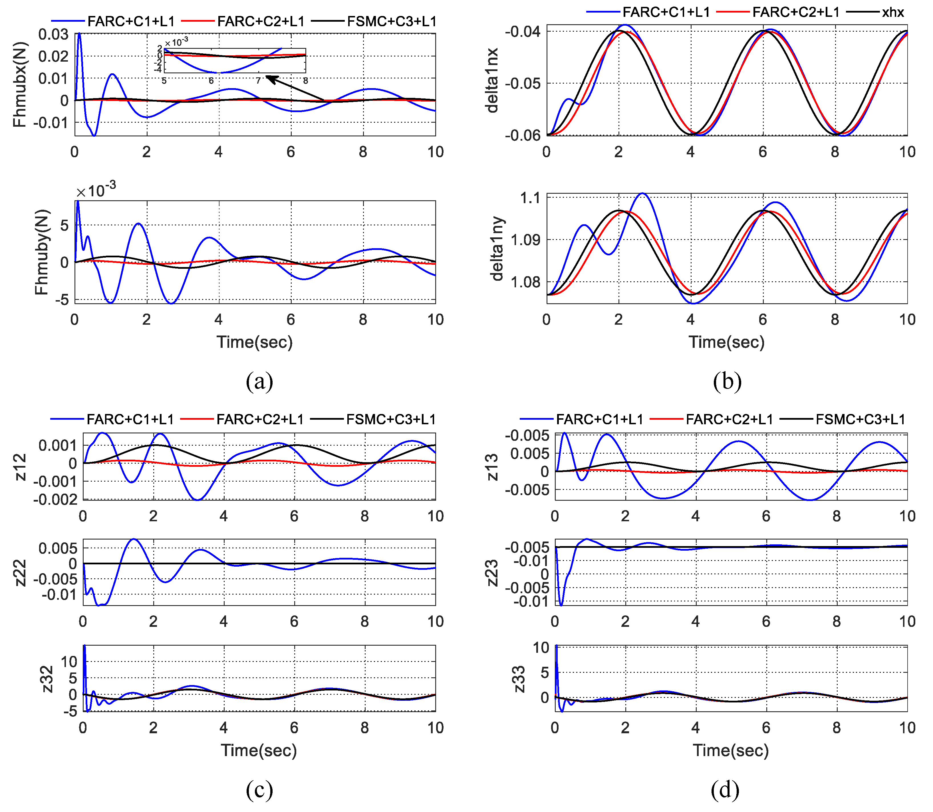
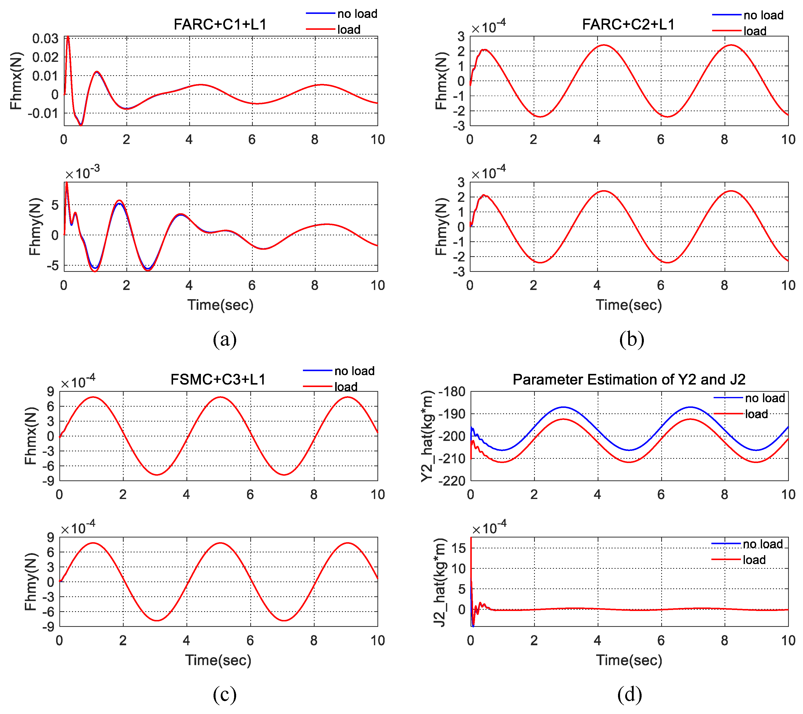
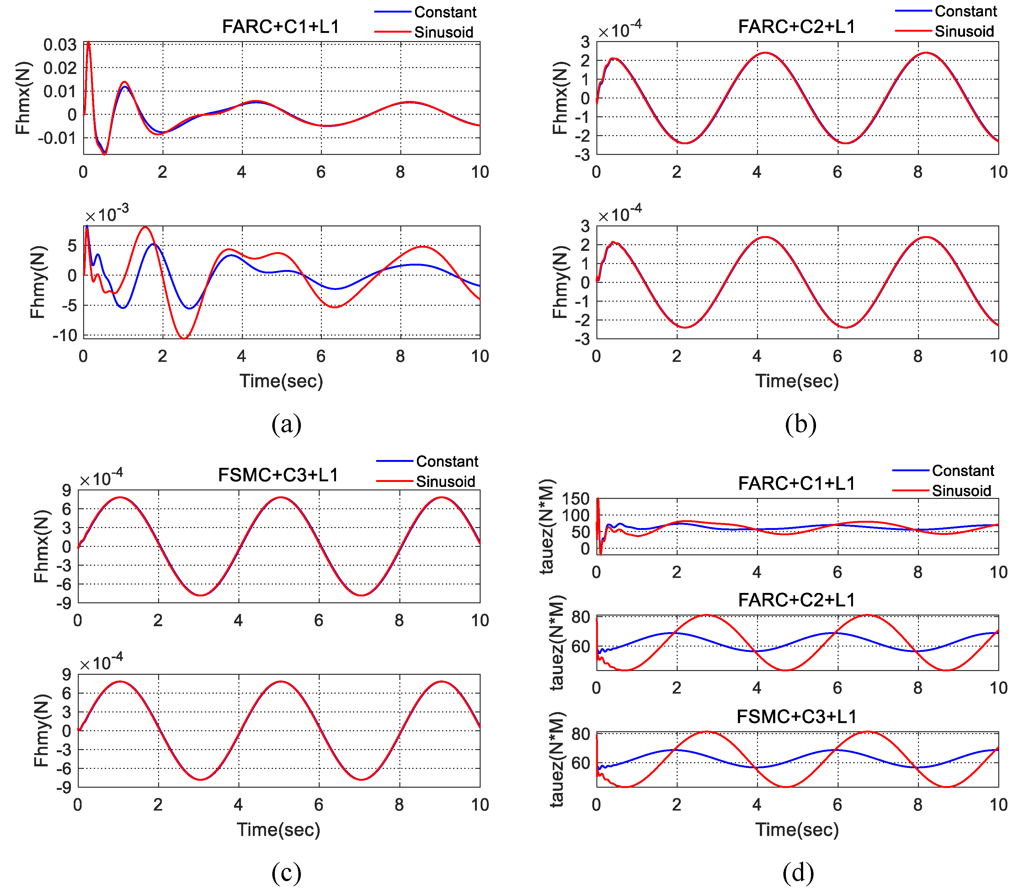
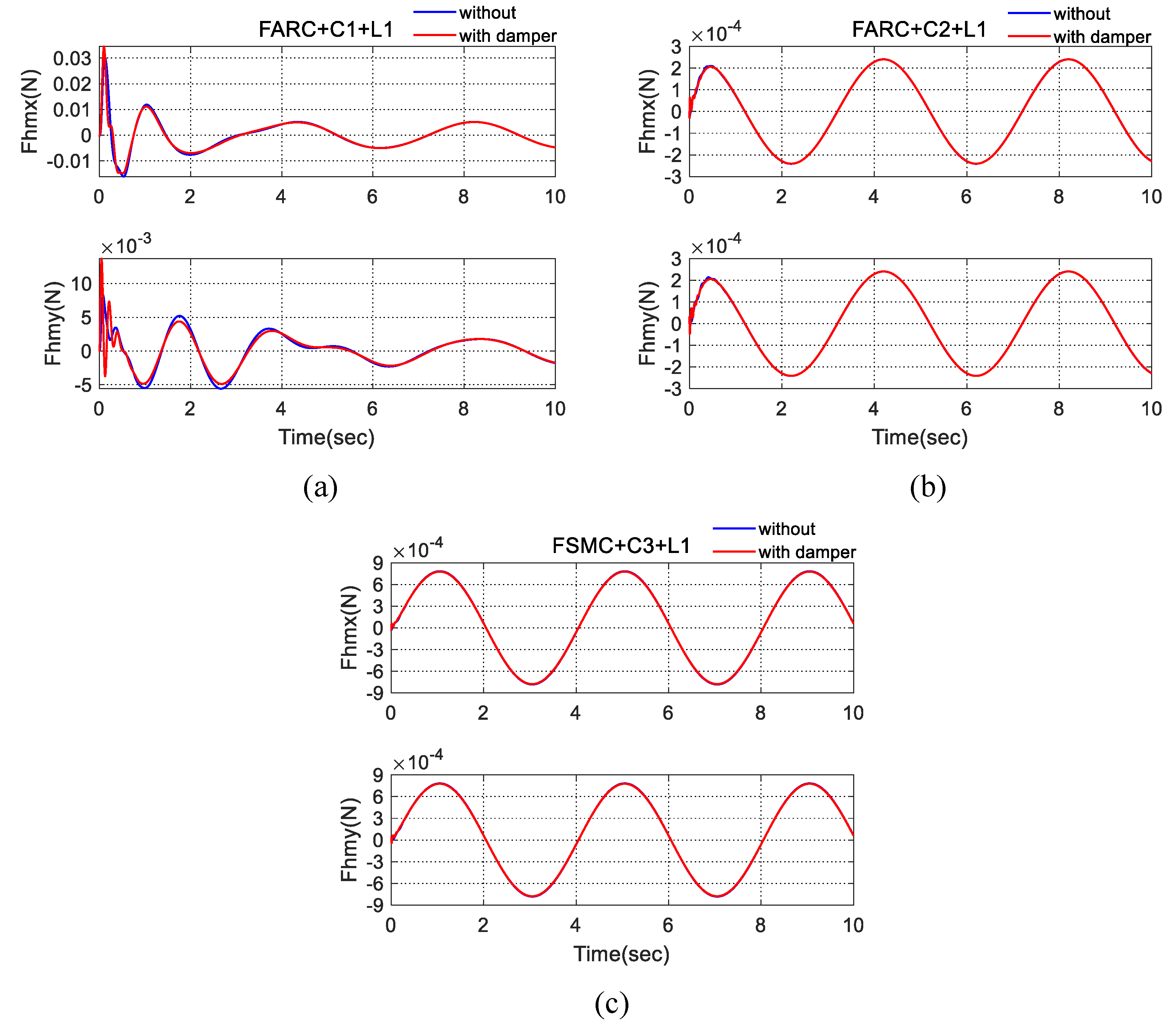
4.2. Simulation Result

In Set1, x e z is selected as x e z = 1.759 . The trajectory for human motion is chosen as x h = 0.0499 + 0.01 s i n π 2 t π 2 , 1.0869 + 0.01 s i n π 2 t π 2 . The human machine interaction force and the parameter estimates are shown in Figure 4. Table 1 represents the simulation results in terms of performance indexes, where [ F h m ] M , [ F h m ] F , L 2 [ F h m ] and u M represent maximal value, final value, the L 2 norm value of interaction force and maximal value for control input, respectively. From Figure 4a, it can be seen that our three level interaction force controller (FARC + C2 + L1) and the sliding mode interaction force controller (FSMC + C3 + L1) can achieve a smaller human machine interaction force at x and y axis than PID interaction force controller (FARC + C1 + L1). It is because the middle level PID motion tracking controller (C1) can only achieve a limited bandwidth due to neglecting the multi-joint coupling and various model uncertainties. In comparison, the proposed middle level adaptive robust motion tracking controller (C2) and middle level sliding mode controller (C3) is a model-based controller which considers the strong coupled dynamics, various parameter uncertainties and modeling errors in the controller design, leading to a higher closed loop bandwidth and better motion tracking performance. With a higher middle loop bandwidth, larger controller gains can be selected in the high-level controller. All these lead to a smaller human–machine interaction force achieved by our interaction force controller (FARC + C2 + L1) and the sliding mode interaction force controller (FSMC + C3 + L1). Compared to sliding mode interaction force controller (FSMC + C3 + L1), the proposed three level interaction force controller (FARC + C2 + L1) adopts online parameter adaptation both in high level and middle level controller. Parameter uncertainties can be learned and compensated more precisely, as shown in Figure 4b, which makes human interaction force become smaller. Figure 4c,d demonstrate the tracking errors in three loops.
In Set2, a 2.72 kg load is added, resulting in parameter uncertainties in θ q . Specifically, the first element of θ q named as Y 2 and the fifth element of θ q named as J 2 change. Table 2 shows the simulation results in terms of performance indexes. Figure 5a–c show that our proposed method (FARC + C2 + L1) and the sliding mode interaction force controller (FSMC + C3 + L1) are both insensitive to load change and can achieve a more consistent force control performance than that of PID interaction force control (FARC + C1 + L1). The reason is that parameter uncertainties (such as stiffness of human machine interface, parameters of hydraulic actuator and load changes, see θ F , θ q , and θ u in (10)) are explicitly considered in the dynamic modeling and can be effectively addressed by robust control. Besides, from Figure 5d, we can see that the online parameter adaptation makes the parameter variation be learned quickly and then be compensated effectively, which helps the proposed three level adaptive robust interaction force controller (FARC + C2 + L1) achieve a smaller human–machine interaction force than that of sliding mode interaction force controller (FSMC + C3 + L1).
In Set3, the angle of exoskeleton back x e z is changed into a sinusoid trajectory x e z = 1.559 + 0.2 s i n π 2 t π 2 . Table 3 shows the simulation results in terms of performance indexes. From Figure 6a–c, it can be seen when a posture trajectory x e z changes, the interaction force in PID controller (FARC + C1 + L1) change a lot while there is little difference for both proposed three level adaptive robust interaction force controller (FARC + C2 + L1) and sliding mode interaction force controller (FSMC + C3 + L1). It is because that the unknown trajectory of exoskeleton back has been explicitly considered in the dynamic modeling (see Δ ˜ 3 a in (9)) and can be effectively addressed by robust control, which leads to a better robust performance for disturbance and modeling errors. Thus, the proposed three level interaction force controller can adapt to different trajectories of x e z and is effective in practical situations. Due to less control input (the ankle joint is passive), the wearer has to provide an additional interaction torque τ e z to make the position of the exoskeleton back be bounded, as shown in Figure 6d. Thus the human machine interaction force around the Z axis cannot be minimized.
In Set4, the human machine interface dynamics is described as a spring-damper model, which means in Equation (1), the modeling errors is described as D ˜ 1 = B hm ( x ˙ h x ˙ e ) where B hm is the damping ratio at the human machine interface. In the simulation, B hm = d i a g { 0.07 , 0.07 } . Table 4 shows the simulation results in terms of performance indexes. From Figure 7, it can be seen that a consistent performance can be achieved for both the proposed three level adaptive robust interaction force controller (FARC + C2 + L1) and the sliding mode interaction force controller (FSMC + C3 + L1) when a human machine interface modeling error is added. For a PID interaction force controller (FARC + C1 + L1), the human interaction force becomes chattering in transient. The reason is that the human–machine interface modeling error has been explicitly considered in the dynamic modeling (see Δ ˜ 1 a in (9)) and can be effectively addressed by robust control while the closed loop bandwidth and parameter adaptation rate of the PID interaction force controller are limited, leading to a poor disturbance rejection performance.

5. Conclusions

In this paper, a three-level high accuracy interaction force controller for a 3DOF underactuated exoskeleton driven by hydraulic cylinders is developed. The system dynamics is changed from a 3DOF underactuated system in joint space to a 2DOF fully actuated system in Cartesian space with holonomic constraint from the wearer. An adaptive robust control algorithm is applied in the three-level interaction force controller design to effectively address the high order nonlinearities of the hydraulic system, various parameter uncertainties as well as modeling errors. Comparative simulation results demonstrate that the principal human–machine interaction force components are minimized and good robust performance to load change and modeling errors can be achieved. The proposed interaction force control algorithm can be applied to single leg exoskeletons for human performance augmentation with passive ankle joint. It can also be used for the control of a fully actuated single leg exoskeleton when the ankle joint actuator fails or be damaged. In the future, we will consider carrying out experiments on a real underactuated exoskeleton platform to further validate the performance of the proposed interaction force controller. We will also extend the proposed interaction force control algorithm to a lower limb hydraulic exoskeleton. Multi-phase dynamic modeling and interaction force control for different walking phases (such as single leg support and double leg support walking phase) will be conducted.

Author Contributions

Conceptualization, S.C. and F.D.; Funding acquisition, S.C.; Investigation, T.H.; Methodology, T.H. and F.D.; Project administration, J.H.; Software, T.H.; Supervision, S.C.; Validation, L.L. and X.T.; Writing—original draft, S.C. and H.L. All authors have read and agreed to the published version of the manuscript.

Funding

This work was supported by National Natural Science Foundation of China under Grant 61803141 and Grant 51905140; and the Fundamental Research Funds for the Central Universities of China under Grant No.PA2020GDSK0090.

Institutional Review Board Statement

Not applicable.

Informed Consent Statement

Not applicable.

Data Availability Statement

The data that support the findings of this study are available from the corresponding author upon reasonable request.

Conflicts of Interest

The authors declare that they have no conflict of interest.

References

  1. Roveda, L.; Savani, L.; Arlati, S.; Dinon, T.; Legnani, G.; Tosatti, L.M. Design methodology of an active back-support exoskeleton with adaptable backbone-based kinematics. Int. J. Ind. Ergon. 2020, 79, 102991. [Google Scholar] [CrossRef]
  2. Ebrahimi, A. Stuttgart Exo-Jacket: An exoskeleton for industrial upper body applications. In Proceedings of the 2017 10th International Conference on Human System Interactions (HSI), Ulsan, Korea, 17–19 July 2017; pp. 258–263. [Google Scholar]
  3. Verdel, D.; Bastide, S.; Vignais, N.; Bruneau, O.; Berret, B. An Identification-Based Method Improving the Transparency of a Robotic Upper Limb Exoskeleton. Robotica 2021, 1–18. [Google Scholar] [CrossRef]
  4. Mauri, A.; Lettori, J.; Fusi, G.; Fausti, D.; Mor, M.; Braghin, F.; Legnani, G.; Roveda, L. Mechanical and control design of an industrial exoskeleton for advanced human empowering in heavy parts manipulation tasks. Robotics 2019, 8, 65. [Google Scholar] [CrossRef] [Green Version]
  5. Copilusi, C.; Ceccarelli, M.; Carbone, G. Design and numerical characterization of a new leg exoskeleton for motion assistance. Robotica 2015, 33, 1147. [Google Scholar] [CrossRef]
  6. Bao, G.; Pan, L.; Fang, H.; Wu, X.; Yu, H.; Cai, S.; Yu, B.; Wan, Y. Academic Review and Perspectives on Robotic Exoskeletons. IEEE Trans. Neural Syst. Rehabil. Eng. 2019, 27, 2294–2304. [Google Scholar] [CrossRef]
  7. Chen, B.; Zi, B.; Qin, L.; Pan, Q. State-of-the-art research in robotic hip exoskeletons: A general review. J. Orthop. Transl. 2020, 20, 4–13. [Google Scholar] [CrossRef]
  8. Aliman, N.; Ramli, R.; Haris, S.M. Design and development of lower limb exoskeletons: A survey. Robot. Auton. Syst. 2017, 95, 102–116. [Google Scholar] [CrossRef]
  9. Hyun, D.J.; Park, H.; Ha, T.; Park, S.; Jung, K. Biomechanical design of an agile, electricity-powered lower-limb exoskeleton for weight-bearing assistance. Robot. Auton. Syst. 2017, 95, 181–195. [Google Scholar] [CrossRef]
  10. Kim, J.Y.; Cho, B.K. Development of a lower limb exoskeleton worn on the front of a human. J. Intell. Robot. Syst. 2019, 96, 49–64. [Google Scholar] [CrossRef]
  11. Liu, Y.; Gao, Y.; Zhu, Y. A Novel Cable-Pulley Underactuated Lower Limb Exoskeleton for Human Load-Carrying Walking. J. Mech. Med. Biol. 2017, 17, 1740042. [Google Scholar] [CrossRef]
  12. Long, Y.; Du, Z.; Chen, C.; Wang, W.; He, L.; Mao, X.; Xu, G.; Zhao, G.; Li, X.; Dong, W. Development and analysis of an electrically actuated lower extremity assistive exoskeleton. J. Bionic Eng. 2017, 14, 272–283. [Google Scholar] [CrossRef]
  13. Kim, H.; Shin, Y.J.; Kim, J. Design and locomotion control of a hydraulic lower extremity exoskeleton for mobility augmentation. Mechatronics 2017, 46, 32–45. [Google Scholar] [CrossRef]
  14. Chaparro-Rico, B.; Castillo-Castañeda, E. Design of a 2DOF parallel mechanism to assist therapies for knee rehabilitation. Ing. E Investig. 2016, 36, 98–104. [Google Scholar] [CrossRef] [Green Version]
  15. Islam, M.R.; Rahmani, M.; Rahman, M.H. A novel exoskeleton with fractional sliding mode control for upper limb rehabilitation. Robotica 2020, 38, 2099–2120. [Google Scholar] [CrossRef]
  16. Lu, R.; Li, Z.; Su, C.Y.; Xue, A. Development and learning control of a human limb with a rehabilitation exoskeleton. IEEE Trans. Ind. Electron. 2013, 61, 3776–3785. [Google Scholar] [CrossRef]
  17. Wang, L.; Du, Z.; Dong, W.; Shen, Y.; Zhao, G. Probabilistic sensitivity amplification control for lower extremity exoskeleton. Appl. Sci. 2018, 8, 525. [Google Scholar] [CrossRef] [Green Version]
  18. Huo, W.; Alouane, M.A.; Amirat, Y.; Mohammed, S. Force control of SEA-based exoskeletons for multimode human–robot interactions. IEEE Trans. Robot. 2019, 36, 570–577. [Google Scholar] [CrossRef]
  19. Chen, L.; Wang, C.; Song, X.; Wang, J.; Zhang, T.; Li, X. Dynamic trajectory adjustment of lower limb exoskeleton in swing phase based on impedance control strategy. Proc. Inst. Mech. Eng. Part I J. Syst. Control Eng. 2020, 234, 1120–1132. [Google Scholar] [CrossRef]
  20. Roveda, L.; Maskani, J.; Franceschi, P.; Abdi, A.; Braghin, F.; Tosatti, L.M.; Pedrocchi, N. Model-based reinforcement learning variable impedance control for human-robot collaboration. J. Intell. Robot. Syst. 2020, 100, 1–17. [Google Scholar] [CrossRef]
  21. Roveda, L.; Haghshenas, S.; Caimmi, M.; Pedrocchi, N.; Molinari Tosatti, L. Assisting operators in heavy industrial tasks: On the design of an optimized cooperative impedance fuzzy-controller with embedded safety rules. Front. Robot. AI 2019, 6, 75. [Google Scholar] [CrossRef] [Green Version]
  22. Zhang, X.; Yin, G.; Li, H.; Dong, R.; Hu, H. An adaptive seamless assist-as-needed control scheme for lower extremity rehabilitation robots. Proc. Inst. Mech. Eng. Part I J. Syst. Control Eng. 2020. [Google Scholar] [CrossRef]
  23. Rosales Luengas, Y.; López-Gutiérrez, R.; Salazar, S.; Lozano, R. Robust controls for upper limb exoskeleton, real-time results. Proc. Inst. Mech. Eng. Part I J. Syst. Control Eng. 2018, 232, 797–806. [Google Scholar] [CrossRef]
  24. Yao, B.; Tomizuka, M. Adaptive robust control of SISO nonlinear systems in a semi-strict feedback form. Automatica 1997, 33, 893–900. [Google Scholar] [CrossRef]
  25. Yao, B.; Tomizuka, M. Adaptive robust control of MIMO nonlinear systems in semi-strict feedback forms. Automatica 2001, 37, 1305–1321. [Google Scholar] [CrossRef]
  26. Chen, S.; Chen, Z.; Yao, B.; Zhu, X.; Zhu, S.; Wang, Q.; Song, Y. Adaptive robust cascade force control of 1-DOF hydraulic exoskeleton for human performance augmentation. IEEE/ASME Trans. Mechatron. 2016, 22, 589–600. [Google Scholar] [CrossRef]
  27. Chen, S.; Chen, Z.; Yao, B. Precision cascade force control of multi-DOF hydraulic leg exoskeleton. IEEE Access 2018, 6, 8574–8583. [Google Scholar] [CrossRef]
  28. Zhu, S.; Jin, X.; Yao, B.; Chen, Q.; Pei, X.; Pan, Z. Non-linear sliding mode control of the lower extremity exoskeleton based on human-robot cooperation. Int. J. Adv. Robot. Syst. 2016, 13. [Google Scholar] [CrossRef]
  29. Liang, C.; Hsiao, T. Admittance Control of Powered Exoskeletons Based on Joint Torque Estimation. IEEE Access 2020, 8, 94404–94414. [Google Scholar] [CrossRef]
  30. Huo, W.; Mohammed, S.; Amirat, Y.; Kong, K. Fast Gait Mode Detection and Assistive Torque Control of an Exoskeletal Robotic Orthosis for Walking Assistance. IEEE Trans. Robot. 2018, 34, 1035–1052. [Google Scholar] [CrossRef]
  31. Choi, B.; Seo, C.; Lee, S.; Kim, B. Control of power-augmenting lower extremity exoskeleton while walking with heavy payload. Int. J. Adv. Robot. Syst. 2019, 16. [Google Scholar] [CrossRef] [Green Version]
  32. Ka, D.M.; Hong, C.; Toan, T.H.; Qiu, J. Minimizing human-exoskeleton interaction force by using global fast sliding mode control. Int. J. Control Autom. Syst. 2016, 14, 1064–1072. [Google Scholar] [CrossRef]
  33. Chen, S.; Han, T.; Dong, F.; Han, J.; Lu, L.; Liu, H. Adaptive Robust Force Control of an Underactuated Stance Leg Exoskeleton for Human Performance Augmentation. In Proceedings of the 2021 IEEE International Conference on Mechatronics (ICM), Kashiwa, Japan, 7–9 March 2021; pp. 1–6. [Google Scholar] [CrossRef]
  34. Deng, W.; Yao, J.; Wang, Y.; Yang, X.; Chen, J. Output feedback backstepping control of hydraulic actuators with valve dynamics compensation. Mech. Syst. Signal Process. 2021, 158, 107769. [Google Scholar] [CrossRef]
  35. Yang, X.; Yao, J.; Deng, W. Output feedback adaptive super-twisting sliding mode control of hydraulic systems with disturbance compensation. ISA Trans. 2021, 109, 175–185. [Google Scholar] [CrossRef] [PubMed]
  36. Lai, X.; Wang, Y.; Wu, M.; Cao, W. Stable control strategy for planar three-link underactuated mechanical system. IEEE/ASME Trans. Mechatron. 2016, 21, 1345–1356. [Google Scholar] [CrossRef]
  37. Zhang, P.; Lai, X.; Wang, Y.; Wu, M. Motion planning and adaptive neural sliding mode tracking control for positioning of uncertain planar underactuated manipulator. Neurocomputing 2019, 334, 197–205. [Google Scholar] [CrossRef]
  38. Yao, B.; Jiang, C. Advanced motion control: From classical PID to nonlinear adaptive robust control. In Proceedings of the 2010 11th IEEE International Workshop on Advanced Motion Control (AMC), Nagaoka, Japan, 21–24 March 2010; pp. 815–829. [Google Scholar]
  39. Li, C.; Chen, Z.; Yao, B. Identification and adaptive robust precision motion control of systems with nonlinear friction. Nonlinear Dyn. 2019, 95, 995–1007. [Google Scholar] [CrossRef]
  40. Roveda, L.; Forgione, M.; Piga, D. Robot control parameters auto-tuning in trajectory tracking applications. Control Eng. Pract. 2020, 101, 104488. [Google Scholar] [CrossRef]
  41. Roveda, L.; Magni, M.; Cantoni, M.; Piga, D.; Bucca, G. Human–robot collaboration in sensorless assembly task learning enhanced by uncertainties adaptation via Bayesian Optimization. Robot. Auton. Syst. 2021, 136, 103711. [Google Scholar] [CrossRef]
  42. Winter, D.A. Biomechanics and Motor Control of Human Movement; John Wiley and Sons: Hoboken, NJ, USA, 2009. [Google Scholar]
Figure 1. 3-DOF underactuated hydraulic exoskeleton.
Machines 09 00096 g001
Figure 2. Overall Control Structure.
Machines 09 00096 g002
Figure 3. The design process of the proposed control.
Machines 09 00096 g003
Figure 4. Simulation results for Set1: (a) human machine interaction force at x and y axis, (b) parameter estimation of Δ 1 a n , (c) three loop tracking errors for knee joint, (d) three loop tracking errors for hip joint.
Machines 09 00096 g004
Figure 5. Simulation results for Set2: (a) human machine interaction force at x and y axis for FARC + C1 + L1, (b) human machine interaction force at x and y axis for FARC + C2 + L1, (c) human machine interaction force at x and y axis for FSMC + C3 + L1, (d) parameter estimation of Y2 and J2.
Machines 09 00096 g005
Figure 6. Simulation results for Set3: (a) human machine interaction force at x and y axis for FARC + C1 + L1, (b) human machine interaction force at x and y axis for FARC + C2 + L1, (c) human machine interaction force at x and y axis for FSMC + C3 + L1, (d) torque provided by the wearer around z axis ( τ e z ).
Machines 09 00096 g006
Figure 7. Simulation results for Set4: (a) human machine interaction force at x and y axis for FARC + C1 + L1, (b) human machine interaction force at x and y axis for FARC + C2 + L1, (c) human machine interaction force at x and y axis for FSMC + C3 + L1.
Machines 09 00096 g007
Table 1. Quantitative Force Control Performance in Set1.
Controller [ F hm ] M ( N ) [ F hm ] F ( N ) L 2 [ F hm ] ( N ) u M ( V )
FARC + C1 + L1 3.04 × 10 2 5.10 × 10 3 5.8 × 10 3 16.15
x axisFARC + C2 + L1 2.41 × 10 4 2.41 × 10 4 1.66 × 10 4 1.52
FSMC + C3 + L1 7.83 × 10 4 7.83 × 10 4 5.54 × 10 4 1.64
FARC + C1 + L1 8.3 × 10 3 8.30 × 10 3 2.5 × 10 3 15.72
y axisFARC + C2 + L1 2.41 × 10 4 2.41 × 10 4 1.66 × 10 4 4.42
FSMC + C3 + L1 7.83 × 10 4 7.83 × 10 4 5.54 × 10 4 4.75
Table 2. Quantitative Force Control Performance in Set2.
Controller [ F hm ] M ( N ) [ F hm ] F ( N ) L 2 [ F hm ] ( N ) u M ( V )
FARC + C1 + L1 3.11 × 10 2 3.11 × 10 3 5.90 × 10 3 16.15
x axisFARC + C2 + L1 2.41 × 10 4 2.41 × 10 4 1.66 × 10 4 0.98
FSMC + C3 + L1 7.83 × 10 4 7.83 × 10 4 5.54 × 10 4 1.11
FARC + C1 + L1 8.7 × 10 3 8.7 × 10 3 2.7 × 10 3 15.72
y axisFARC + C2 + L1 2.41 × 10 4 2.41 × 10 4 1.66 × 10 4 2.97
FSMC + C3 + L1 7.83 × 10 4 7.83 × 10 4 5.54 × 10 4 3.30
Table 3. Quantitative Force Control Performance in Set3.
Controller [ F hm ] M ( N ) [ F hm ] F ( N ) L 2 [ F hm ] ( N ) u M ( V )
FARC + C1 + L1 3.12 × 10 2 3.12 × 10 2 6.2 × 10 3 16.15
x axisFARC + C2 + L1 2.41 × 10 4 2.41 × 10 4 1.66 × 10 4 1.69
FSMC + C3 + L1 7.84 × 10 4 7.84 × 10 4 5.54 × 10 4 1.82
FARC + C1 + L1 1.06 × 10 2 1.06 × 10 2 4.2 × 10 3 15.72
y axisFARC + C2 + L1 2.41 × 10 4 2.41 × 10 4 1.66 × 10 4 5.19
FSMC + C3 + L1 7.84 × 10 4 7.84 × 10 4 5.54 × 10 4 5.52
Table 4. Quantitative Force Control Performance in Set4.
Controller [ F hm ] M ( N ) [ F hm ] F ( N ) L 2 [ F hm ] ( N ) u M ( V )
FARC + C1 + L1 3.45 × 10 2 3.45 × 10 2 5.6 × 10 3 16.15
x axisFARC + C2 + L1 2.41 × 10 4 2.41 × 10 4 1.66 × 10 4 1.52
FSMC + C3 + L1 7.78 × 10 4 7.78 × 10 4 5.50 × 10 4 1.64
FARC + C1 + L1 1.37 × 10 2 1.37 × 10 2 2.4 × 10 3 15.72
y axisFARC + C2 + L1 2.41 × 10 4 2.41 × 10 4 1.66 × 10 4 4.42
FSMC + C3 + L1 7.78 × 10 4 7.78 × 10 4 5.50 × 10 4 4.75
Publisher’s Note: MDPI stays neutral with regard to jurisdictional claims in published maps and institutional affiliations.

