
PFC-Based Control of Friction-Induced Instabilities in Drive Systems

1
Institute for Automation Engineering, Otto von Guericke University Magdeburg, 39106 Magdeburg, Germany
2
Department of Electric Power Systems, National Research University “Moscow Power Engineering Institute”, 111250 Moscow, Russia
*
Author to whom correspondence should be addressed.
Machines 2021, 9(7), 134; https://0-doi-org.brum.beds.ac.uk/10.3390/machines9070134
Submission received: 22 June 2021
/
Revised: 9 July 2021
/
Accepted: 13 July 2021
/
Published: 16 July 2021
(This article belongs to the Special Issue Advances in Electric Machines and Associated Drives for More Electric Transportation (Aircraft, Automotive, Rail and Marine))
Abstract
:This paper is concerned with control-based damping of friction-induced self-excited oscillations that appear in electromechanical systems with an elastic shaft. This approach does not demand additional oscillations measurements or an observer design. The control system provides the angular velocity and damping control via the combination of a parallel feed-forward compensator (PFC) and adaptive -tracking feedback control. The PFC is designed to stabilize the zero dynamics of an augmented system and renders it almost strict positive real (ASPR). The proposed control approach is tested in simulations.
1. Introduction
A number of friction effects appear in different machines and mechanisms driven by automated electric drive systems. It is well known that friction may deteriorate performance of feedback control loops. This may also result in oscillatory dynamics and large steady-state errors during closed-loop operation and typically leads to increased mechanical wear [1,2,3,4]. Friction characteristics with dropping regions are particularly negative, i.e., negative slope regions of friction torque-velocity characteristics. Here, by operation in these regions, friction-induced stick-slip or self-excited oscillations may appear. This problem is common for various areas: cranes, rolling mills, industrial robots, railways, vehicles, aircraft engines, rolling element bearings, drilling systems, etc. [5,6,7,8,9,10,11,12]. To solve the problem of these nonlinear oscillations, a number of control-based approaches have been presented in the literature, e.g., PD control [13,14], linear robust control [15], indirect adaptive control [16], feedback linearization [17], sliding-mode control [18], and backstepping control [19]. In the majority of the works, it is considered that oscillations in a working element of the mechanism or machine can be measured or estimated.
In this paper, a new approach for damping the friction-induced self-excited oscillations is proposed. This approach does not require an additional measurement system on the working element side and can be easily integrated in classical motion control systems without their full redesign. This makes this method valuable from a practical point of view. The proposed control system is based on a combination of a parallel feed-forward compensator (PFC) and -tracking controller. Its effectiveness is verified using the simulation model. The problem of friction-induced self-excited vibrations is studied on the example of a two-mass electromechanical system with an elastic shaft. The system is considered to be driven by an electric drive. It will be shown that, during operation in the negative slope region, not only the system dynamics becomes unstable, but its zero dynamics becomes unstable too, i.e., the nonminimum phase. From a theoretical point of view, application of feedback control to this class of systems is a challenging task, as they are known to be unstable under high controller gains. In order to provide stability of the closed-loop system, at first, parallel feed-forward interconnection of a plant and compensator [20,21,22,23,24] is applied, which results in an augmented system with a redefined output and stable zero dynamics. After this, the augmented system dynamics is stabilized applying adaptive -tracking control [25]. It should be mentioned that the proposed PFC design also renders the augmented plant almost strict positive real (ASPR) [23,24], hence the basis for other control approaches as well.
Section 2 presents the distributed parameter mathematical model of the two-mass electromechanical system with an elastic shaft and its discretization. In Section 3, the problem of occurrence of friction-induced self-excited vibrations is shown. Section 4 introduces the design of a PFC and control law. In Section 5, the proposed control system is evaluated in a simulation study. Section 6 summarizes the results presented in this paper and gives an outlook for future work.
2. Modeling
2.1. Mathematical Model
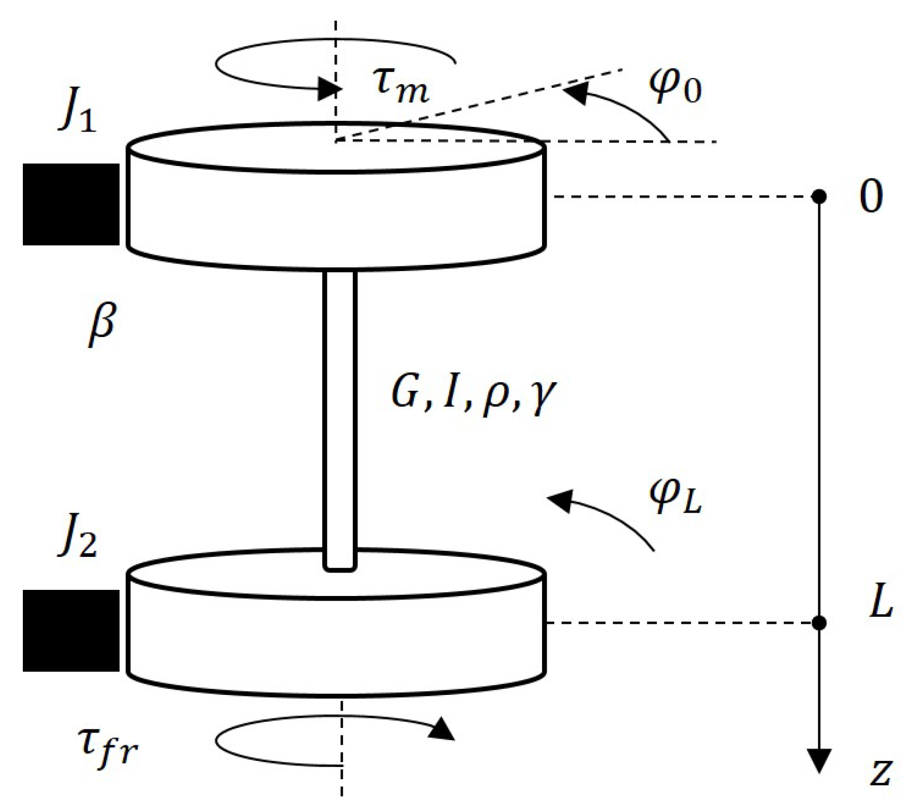
In this contribution, a prototypic rotatory two-mass electromechanical system with an elastic shaft, as illustrated in Figure 1, is considered [12,26]. Here, the drive torque actuates the first mass and the load friction torque is subjected to the second mass. The electromechanical system can be described by the following hyperbolic partial differential equation (PDE)
with two boundary conditions
Here, is the rotational angle of the shaft, which depends on the spatial coordinate and time t, is the rotational angle of the first mass, i.e., the motor, is the rotational angle of the second mass, and are the first and second masses’ moments of inertia, is the coefficient of viscous friction subjected to the first mass, G and I are the shear modulus and the moment of inertia of the shaft, and and are the density and structural damping of the shaft. The prime and dot symbols denote the spatial and time derivatives, respectively.
In this contribution, friction load curves possessing a negative slope region are of particular interest as they may cause instability and the occurrence of limit cycles. Therefore, the following friction model is utilized [1]
where is the Coulomb friction torque, is the viscous dissipation torque, is the static friction torque, is the empirical parameter characterizing the Stribeck effect, is the adjustable parameter of the slope in the region of zero velocity.
It is assumed that the electric drive operates in the current (torque) control mode. Its fast closed-loop dynamics can be typically neglected, and, thus, the motor torque can be considered as a control input .
2.2. Model Discretization
For simulation and control design, the presented infinite-dimensional electromechanical model is discretized. Here, the method of lines has been applied [27]. Therefore, the spatial coordinate of the PDE (1) is discretized by applying a finite difference approximation with grid points
where is the distance between two grid points and is the value of at grid node i.
Substituting the approximations (5) and (6) into (1)–(3) and solving the equations with respect to their highest time derivatives, the following matrix equation results
Here, the stiffness , damping , control input , and friction torque matrices are calculated as follows:
where
By defining the additional angular velocity vector and the state vector , the electromechanical system can be represented in state-space as follows:
where , , are the associated system matrices, and is the identity matrix.
Considering the angular velocity of the first mass as the measured output signal , the output equation yields
where is the corresponding output matrix.
In order to perform linear analysis and control design, the high-order nonlinear model (8) and (9) can be linearized for a fixed slope of the friction curve as follows:
Here, the system matrix comprises a new damping matrix , which replaces R. This matrix is calculated in the same way as R with a new boundary damping coefficient
The model parameters used for simulations are summarized in Table 1. The presented dynamic models are implemented in Matlab and calculated using the variable-step solver.
3. Friction-Induced Self-Excited Oscillations
3.1. Stability and Zero Dynamics
The relative degree and zero dynamics of a system are important properties for control design. For the single-input single-output linear time-invariant system
the relative degree can be obtained as the difference between the denominator and numerator polynomials orders of the transfer function
or as the smallest positive number which satisfies
The concept of zero dynamics for a linear system is equivalent to the zeros of the associated transfer function [28]. The location of the zeros in the complex plane determines the stability of the zero dynamics. The system is known to be (strictly) minimum phase if the zeros of are in the left-half plane (LHP) ().
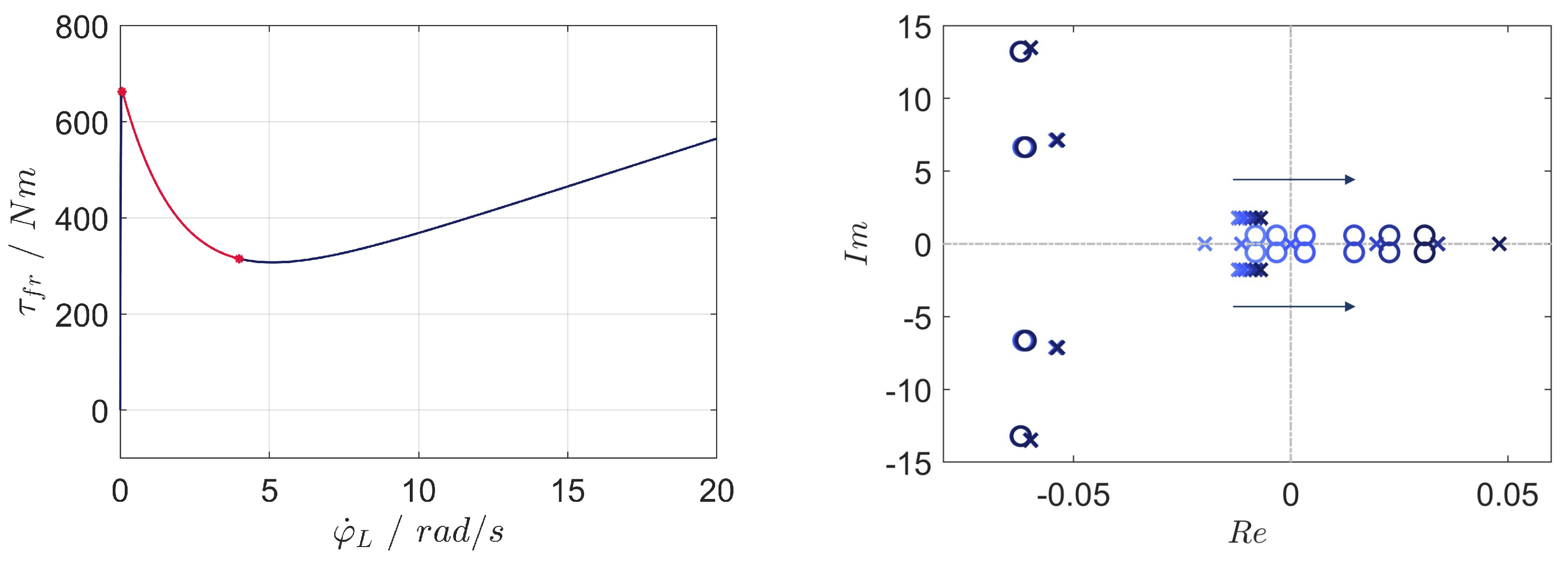
From a theoretical point of view, the source of instability and nonminimum phase in the model (10) and (11) is the appearance of a negative slope coefficient for certain regions of the friction loading curve. In Figure 2 (left), the friction curve with Stribeck effect (4) is illustrated. Here, the negative slope region can be seen for small angular velocities up to 5 rad/s.
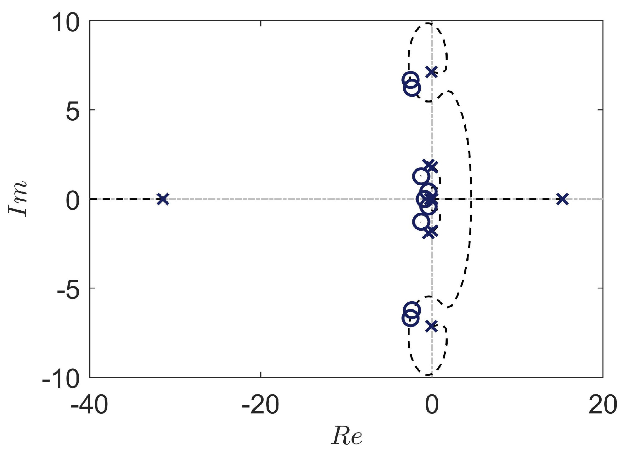
To analyze the stability of the open-loop linear plant and its zero dynamics (10) and (11), the pole-zero maps for varying slope coefficients are obtained and represented in Figure 2 (right). Here, it can be seen that the slope variation has a strong impact on the location of one real pole and one low-frequency complex conjugated pair of poles and zeros, while the dynamics of the higher-frequency modes is not affected. The low-frequency complex zero pair moves into the right-half plane (RHP), i.e., the system becomes nonminimum phase, for small slopes coefficients . It can be also seen that the real pole moves into the RHP for resulting in unstable system dynamics. As depicted in Figure 2 (left, red), the region of unstable operating points is rad/s.
3.2. Conventional Velocity Control
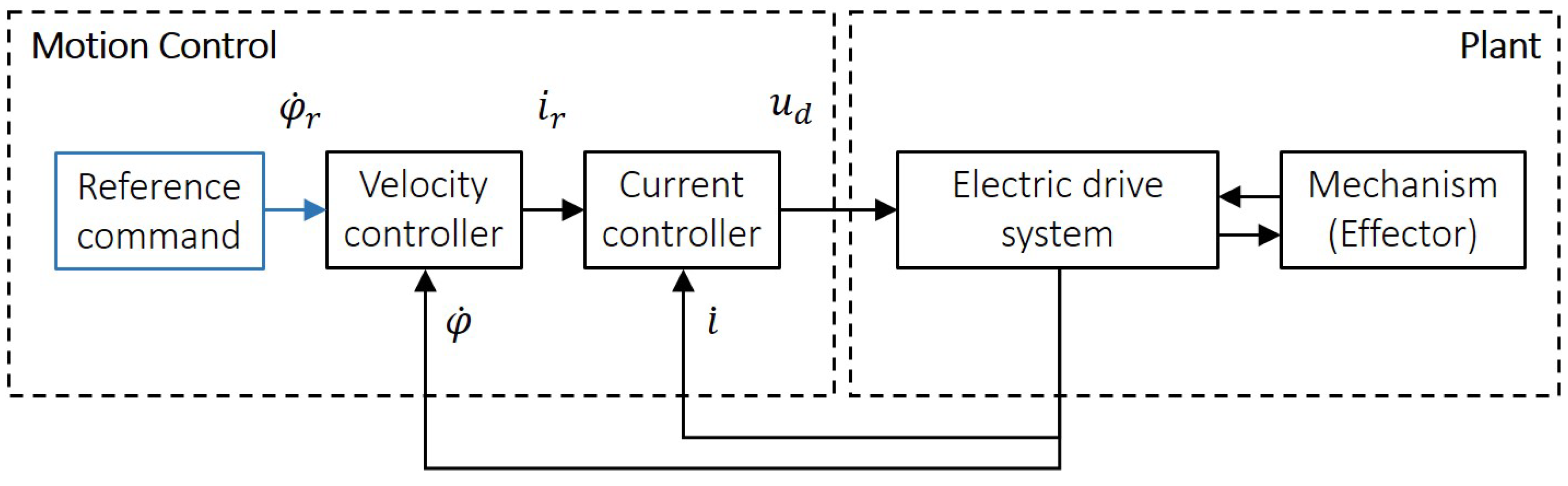
Currently, most modern mechanisms and machines are equipped with automated electric drive systems. Manufacturers of those systems typically offer a complex product with an individual software solution, e.g., a power converter with a fully parameterizable motion control system. Velocity control is one of the typical tasks for industrial systems. Due to simplicity in design and high robustness, the cascade control scheme with -controllers, depicted in Figure 3, have found wide practical application. Direct velocity measurements on the effector of the mechanism are often complicated and involve additional costs. Alternatively, they can be provided on the motor shaft via incremental or optical sensors. Therefore, for the presented system it means that only the first mass angular velocity is measured. From a theoretical point of view, this choice of system output for systems with more than one masses and distributed states induces zero dynamics [28]. As has been illustrated in Figure 2 (right), for systems operating in the negative slope region of a friction curve problems of unstable zero dynamics may occur.
To show the significance of the zero dynamics problem, the stability properties of the linearized system (10) and (11) with conventional velocity -controller
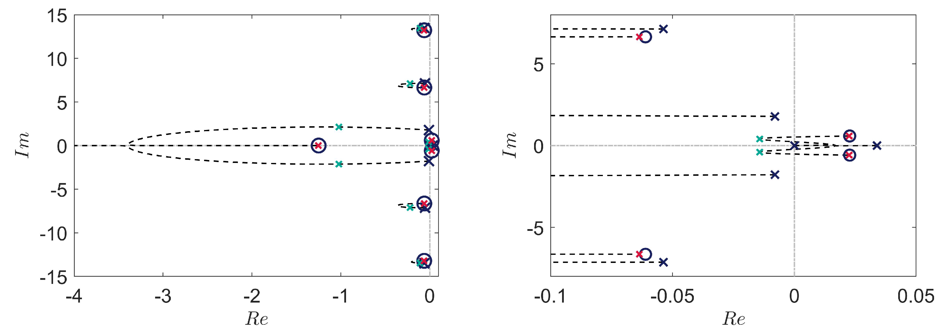
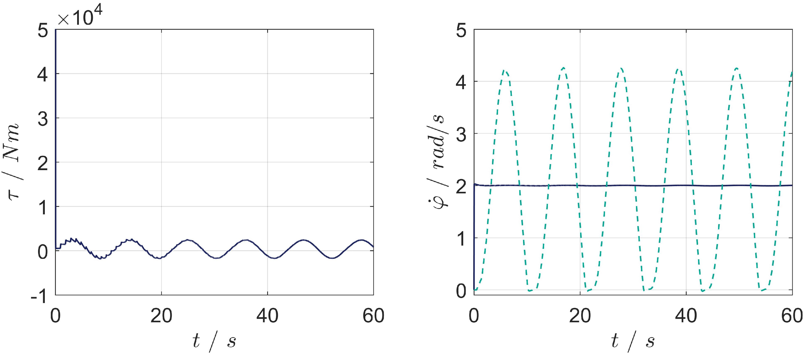
has been studied. Here, the electromechanical system is assumed to be operated at a operating velocity rad/s with a slope coefficient . The open-loop system in this configuration has a relative degree . In Figure 4, the low-frequency part of the root locus for fixed integral time constant s and varying gain is illustrated. Here, from Figure 4 (right), it can be seen that the angular velocity output and internal system dynamics can be asymptotically stabilized for a range of gains . However, this gain tuning yields poor closed-loop dynamics, as shown via simulations of the nonlinear system (Figure 5) for (Figure 4, green poles). For higher gains, e.g., , the system poles are further attracted to the system zeros (Figure 4, red poles) resulting in unstable system dynamics. This instability is a local property for the linearized system, resulting more globally in a limit cycle, i.e., nonlinear oscillations. These friction-induced self-excited oscillations can be seen in Figure 6. Here, application of a high gain leads to an approximate poles-zero pairs cancellation, which results in a stabilized angular velocity for the first mass . However, due to presence of the unstable zero dynamics, the oscillations of the second mass velocity occur.
4. PFC-Based Control
4.1. Motivation
As has been discussed above, friction loads in electromechanical systems may cause significant problems for conventional motion control systems, which can result in instabilities and the occurrence of undesired nonlinear oscillations. This is due to their nonminimum phase behavior or the unstable zero dynamics, which are invariant to feedback and introduce limitations to the achievable closed-loop behavior.
Classical solution approaches to overcome this problem are the redesigning of the control scheme, to find another input–output configuration or to apply observer-based state feedback. In this contribution, a different solution based on a PFC is proposed. This approach is based on an output redefinition and it does not require additional measurements nor an observer design.
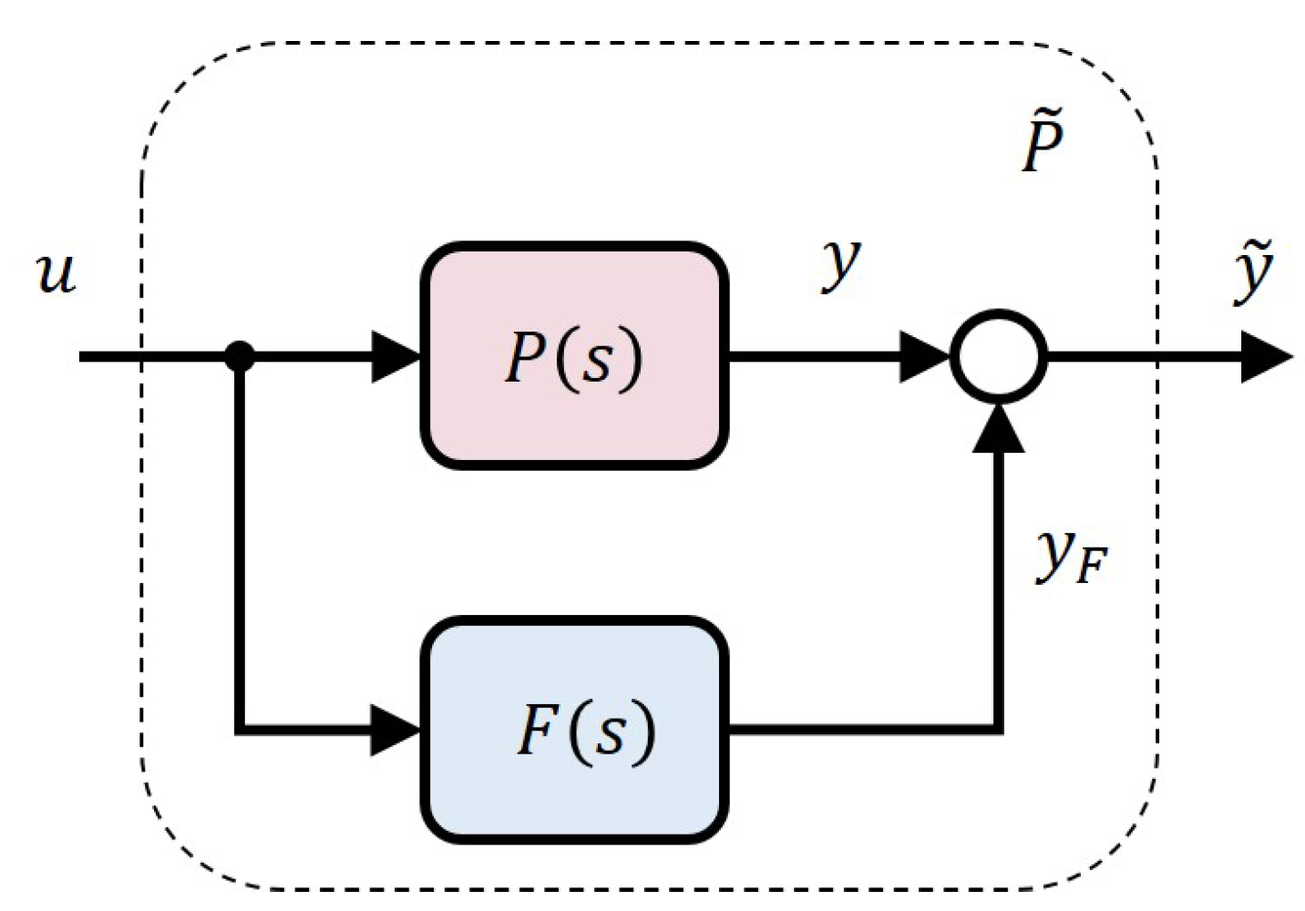
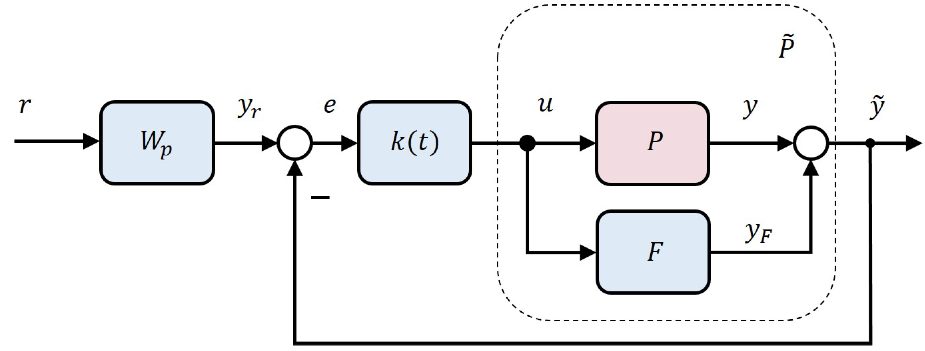
The idea of PFC-based control is to extend the plant of interest P with a PFC F, which achieves desired properties for the augmented plant , e.g., full relative degree, passivity, ASPR. This combination yields a new output (Figure 7), which is considered for further output feedback control design.
In this work, the PFC is designed to achieve ASPR properties [23,24] for the augmented system. Here, for the extended system transfer function , the following conditions should hold:
- is strictly the minimum phase, i.e., zeros of are in the LHP ;
- the relative degree of the system is 0 or 1.
It should be emphasized that the extended plant transfer function can be unstable. However, due to the ASPR properties, it is always stabilizable by proportional output feedback with a sufficiently high gain. This concept is particularly useful for non-identifier-based adaptive control methods, e.g., -tracking control, where the stable zero dynamics plays a key role.
4.2. PFC Design
Consider the following single-input single-output linear time-invariant plant, which is a nonminimum phase and unstable
where is a polynomial of degree d and is a polynomial of degree .
To place the system zeros for the augmented system with the output , an appropriate PFC , as illustrated in Figure 7, has to be designed. In addition, the PFC should not introduce a static contribution in this output.
Consider the following PFC transfer function
where is a polynomial of degree d and is a polynomial of degree , which contains the derivative to achieve a vanishing static contribution.
A parallel feed-forward interconnection of the plant and PFC results in
Here, stability of the system zeros for the extended system is obtained if and only if the numerator polynomial has roots only in LHP. This problem can be directly solved by equating the numerator polynomial to a desired polynomial of a suitable degree
and finding the corresponding coefficients of and . The linear Diophantine Equation (20) can be solved, e.g., by applying Sylvester’s matrix approach [29].
The specific choice of is a degree of freedom in this design. Generally, it should contain only LHP roots with a desired location in the complex plane. The degree of should be selected based on the relative degree of the transfer function , i.e.,
It can be seen that this design achieves for the augmented plant the following relative degree
4.3. Stability of the Augmented Plant
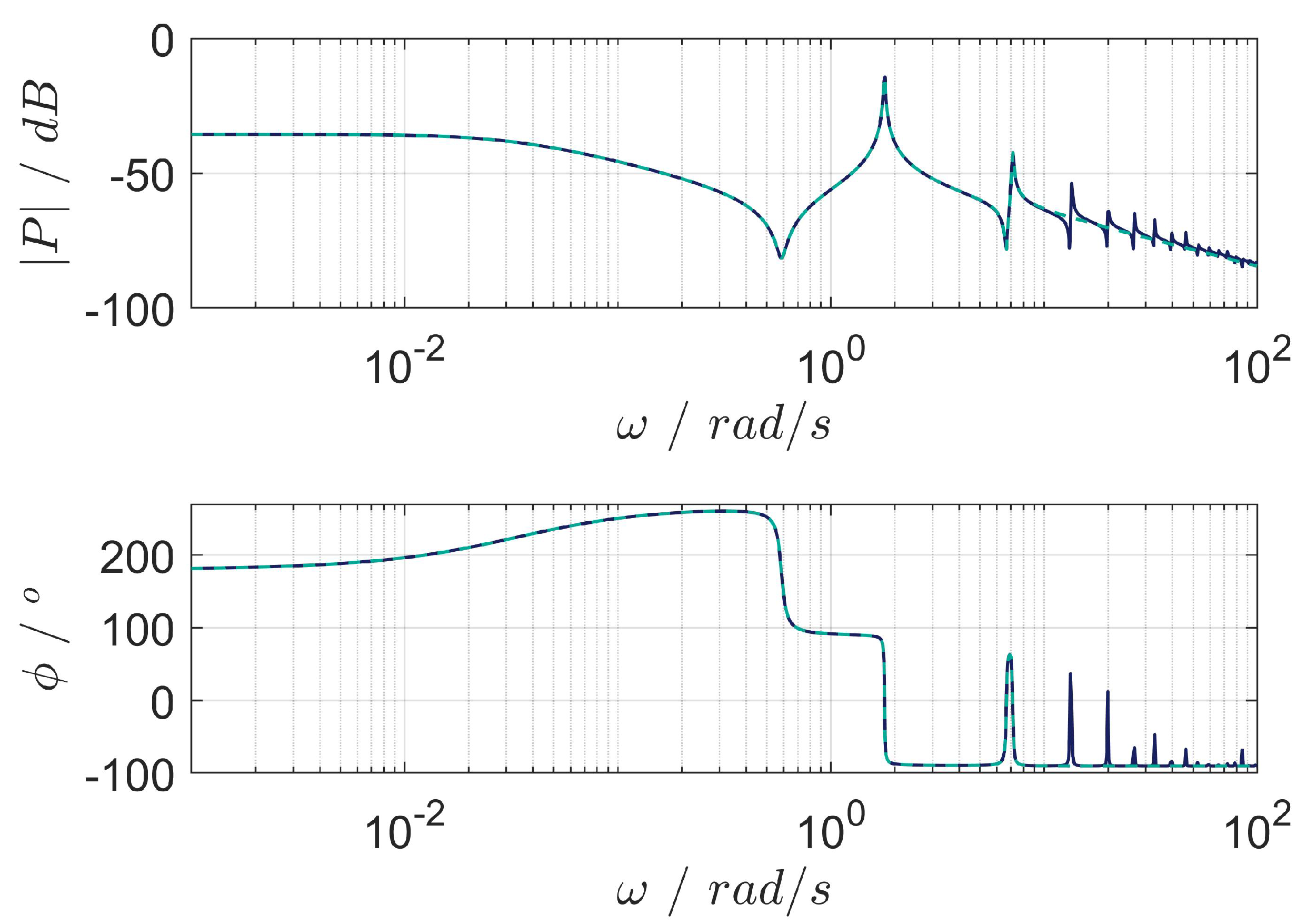
Applying the proposed design procedure yields a PFC of the same order as the plant. The order of the linearized system (10) and (11) depends directly on the number of discretization points n and is typically high. This makes computation and further practical implementation difficult. To overcome this problem, the order of the system or PFC has to be reduced. In this work, the modal truncation procedure has been applied to the high-order plant model [30]. The reduction order selection always depends on the specific application case and can be motivated using the frequency domain. In Figure 8, the Bode diagram of the linearized system is presented (blue). Here, it can be seen that mainly one unstable real pole and two low-frequency eigen-modes have a dominant impact on the system dynamics. Assuming that the higher-frequency modes are not excited by the drive system or external disturbances, a fifth-order model approximation is chosen (green).
To design an appropriate PFC, according to (21), a desired polynomial of degree 9 should be assigned. The numerator polynomial contains the plant polynomials and . Thus, the choice of the desired roots can be motivated physically. Here, the frequencies of and have been left unchanged. However, additional damping for the complex conjugated roots has been added. Additionally, a new location for the real root in LHP has been assigned.
Then, according to (20), the following PFC is obtained
To analyze the linear system properties of and stability of the closed-loop system, the root locus for varying gain is calculated and depicted in Figure 9. It can be seen that applying high gains results in stable closed-loop dynamics. It should be emphasized that the leading coefficient of the resulting augmented plant is negative, and for the root locus and further adaptive control an additional negative sign as multiplier for and is used, respectively.
4.4. PFC-Based Adaptive Feedback Control
To provide stability of the augmented system, an adaptive -tracking control law is used in this work. This approach is not based on a model and requires only minimal information about the system, in particular its DC gain. However, it is only applicable for certain classes of systems, including ASPR systems [20,25].
In Figure 10, the overall control scheme is presented. Here, the tracking error considering the augmented output is
To control the augmented system, the following adaptive control law is applied to the augmented plant
where the time-varying gain is given by the parameter adaptation law
Here, defines the adaptation dead-zone, i.e., the control gain is adapted only if , is the adaptation rate parameter and is the initial value of .
To reduce overshoots in the angular velocities , an additional first order precompensator is utilized
where is a time constant.
5. Results
In this section, the presented PFC-based adaptive -tracking control is evaluated in a simulation study. To verify in particular its robustness with respect to measurement noise and parameter uncertainties, the following simulation scenarios are considered
- Scenario 1: adaptation, angular velocity reference tracking and disturbance rejection of the closed-loop system;
- Scenario 2: adaptation and angular velocity reference tracking of the closed-loop system in the presence of measurement noise;
- Scenario 3: adaptation and angular velocity reference tracking of the closed-loop system in the presence of parameters variation.
The PFC (24) and the following parameters of the feedback control law ((26)), (27) have been utilized and applied to the discretized high-order nonlinear model ((8), (9))
- is chosen as from the reference value rad/s;
- is chosen to provide a reasonable adaptation rate;
- ;
- s for the reference tracking ( s for the adaptation).
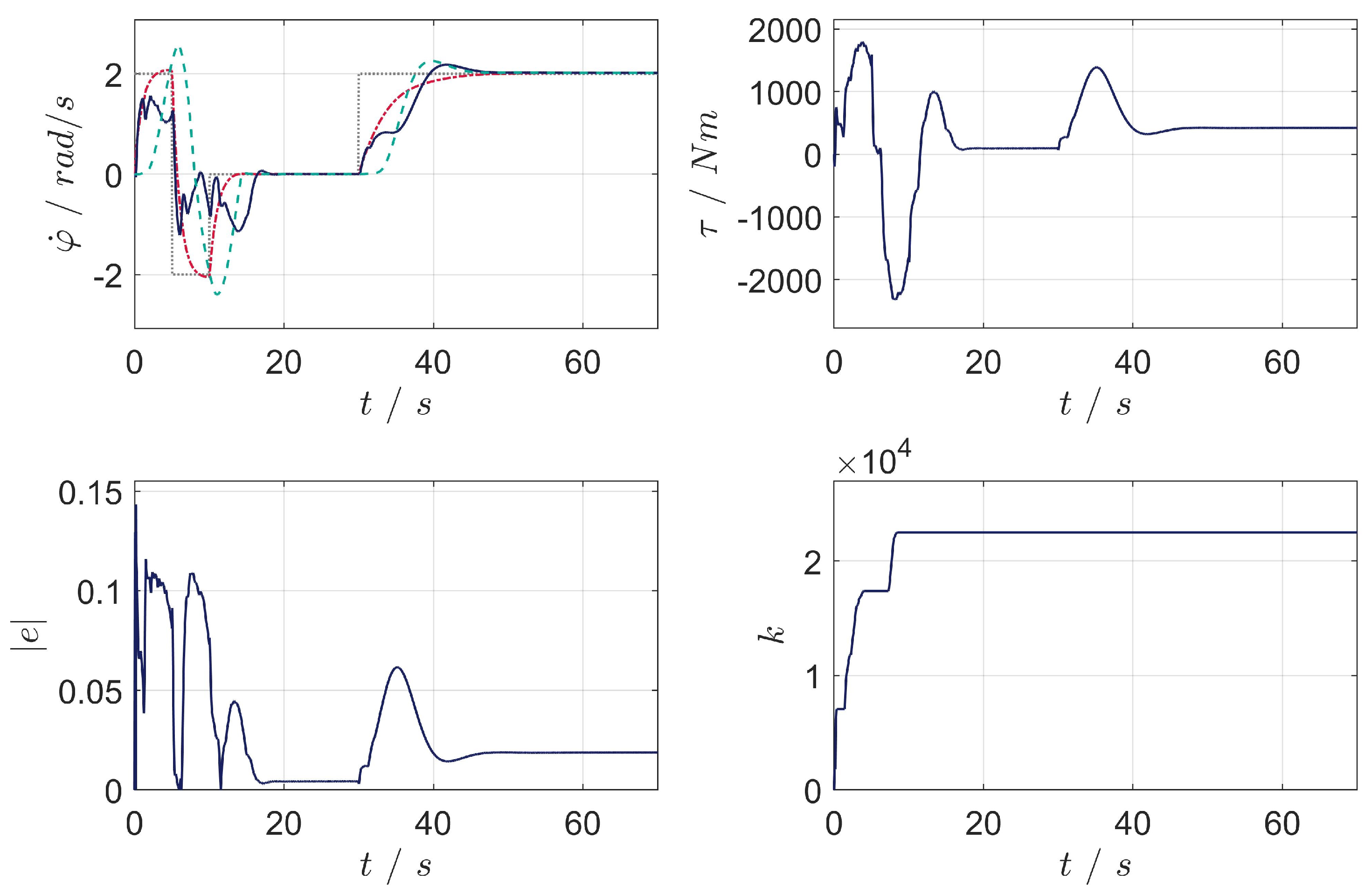
To perform the adaptation and reference tracking, the reference signal r depicted in Figure 11 (dotted gray) has been utilized for all scenarios. Initially, two pulse signals with an amplitude of 2 rad/s and width 5 s are applied to allow for an adaptation of the control gain ( s). After that, at time 30 s, a step signal is applied to evaluate the reference tracking of the closed-loop system ( s).
The following performance measures are considered to evaluate transients during the reference tracking: rise time to 98% of the reference value, settling time with accuracy 2% and relative overshoot. These measures are applied to the angular velocities of the first and second masses.
5.1. Scenario 1
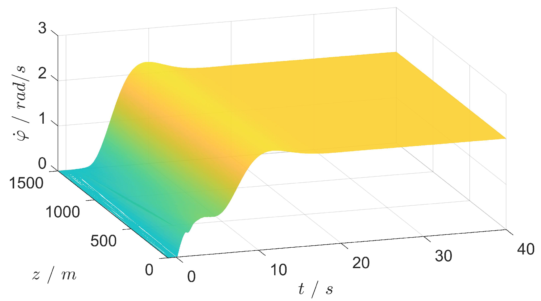
The obtained simulation results are illustrated in Figure 11, Figure 12 and Figure 13. From Figure 11, it can be seen that the absolute value of the control error converges to the prescribed after about 8.5 s resulting in an adapted control gain . The augmented output reaches the reference angular velocity value 14.2 s after the step and settles without overshoot. The performance measures of the reference tracking are summarized in Table 2 and Table 3 (Case 1). From Figure 12 it can be seen that not only the angular velocities on the boundaries and are stabilized, but also the distributed state itself.
5.2. Scenario 2
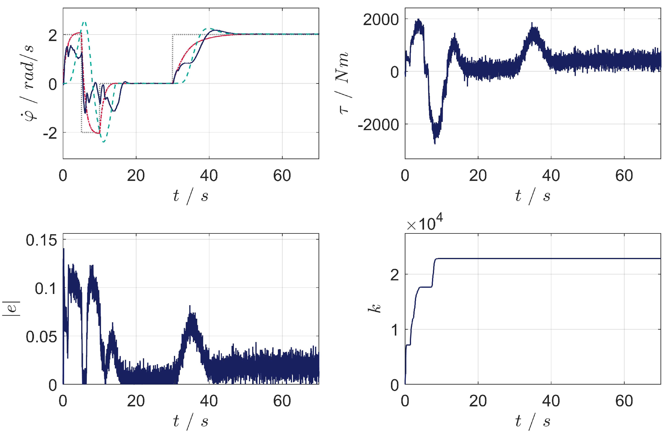
In this scenario, the control law adaptation and reference tracking in the presence of measurement noise are shown. To introduce the measurement noise, a Gaussian distributed random signal with variance of is utilized. The noise is applied to the measured angular velocity on the first mass . The obtained results are illustrated in Figure 14. Here, it can be seen that application of the noise does not deteriorate the adaptation of the control gain . In general, the measurement noise is evaluated from the transient response of and the corresponding parameter is chosen. It should be also emphasized that the high control gains boost the measurement noise considerable. This typically results in faster wear of the actuator and reduced performance [31]. To overcome this problem, an additional low-pass filter for noise signals with a larger variances is needed.
5.3. Scenario 3
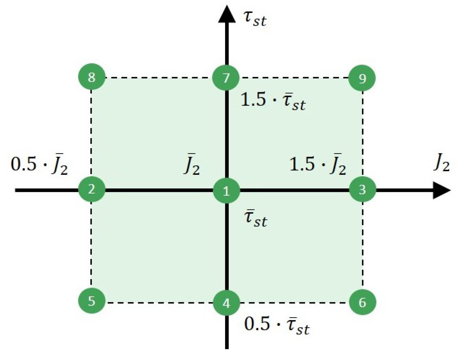
In this scenario, evaluation of the robustness with respect to parameter uncertainties is shown. To introduce the parameter uncertainties, the following parameters variation are considered:
- The static friction torque from (4) is varied in a range of ±50% from its nominal value resulting in a different slope of the friction curve in the operating point of interest;
- The moment of inertia of the second mass is varied in a range of ±50% from its nominal value.
The domain of uncertain parameters is illustrated in Figure 15. Here, the nominal and worst cases of parameter variations are denoted with numbers. The nominal case 1 and following worst cases 2–9 have been used for the simulation study.
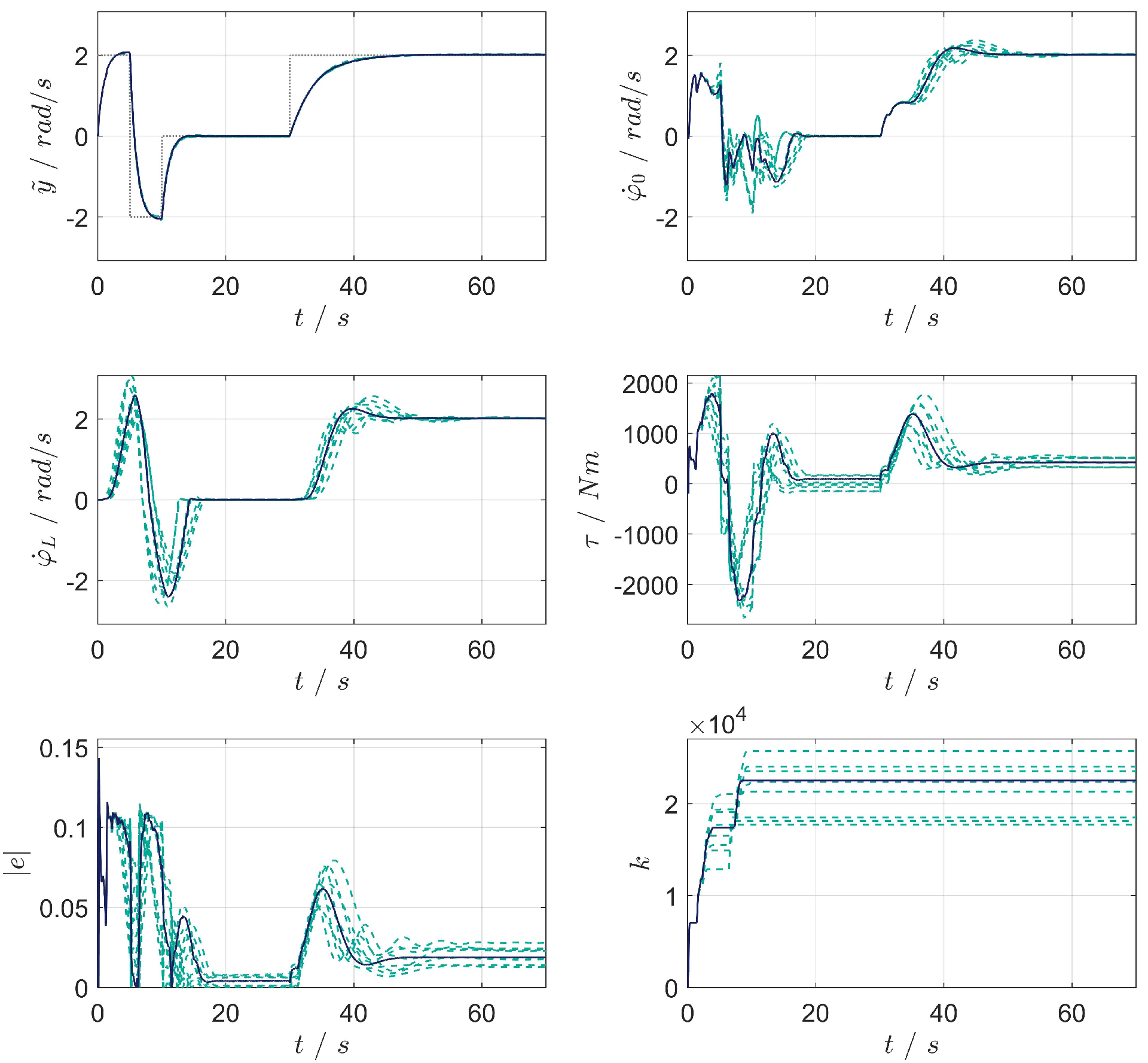
Assuming the model parameters are varying according to cases 2–9 and the control system parameters designed for the nominal case 1 remain constant, the following results are obtained and depicted Figure 16. Here, it can be seen that although in certain cases the performance of the transients has slightly deteriorated, the closed-loop system is always stable. From a theoretical point of view, this means that the designed PFC provides stability of the zero dynamics even for these worst case variations and, hence, the overall control system is robust to these parameter variations. The performance measures of the reference tracking for all cases are summarized in Table 2 and Table 3.
6. Conclusions
In this contribution, the PFC-based adaptive -tracking control is proposed for velocity control of an electromechanical system with friction load. The mathematical model of a two-mass electromechanical system with an elastic shaft and a friction load with the Stribeck effect has been studied. It has been shown that under certain conditions the system becomes a nonminimum phase and unstable. Practically, applying a conventional control system may result in the occurrence of friction-induced self-excited oscillations. To overcome this problem without additional measurements nor observers, an alternative approach based on a PFC has been introduced. The proposed PFC design renders the augmented plant ASPR, i.e., stable zero dynamics and a relative degree of one. Further application of the adaptive -tracking controller results in stable closed-loop system dynamics. The performance of the proposed control system has been successfully evaluated in a simulation study.
In this work, the robustness of the proposed approach is analyzed in the simulation study. For further applications, a robust PFC design that takes into account model uncertainties will be proposed. In addition, the future work will be concerned with a practical verification of the proposed approach.
Author Contributions
Conceptualization, S.P.; methodology, S.P.; software, I.G.; validation, I.G. and S.P.; formal analysis, I.G. and S.P.; investigation, I.G. and S.P.; data curation, I.G.; writing—original draft preparation, I.G.; writing—review and editing, S.P.; visualization, I.G.; supervision, S.P. All authors have read and agreed to the published version of the manuscript.
Funding
This research received no external funding.
Data Availability Statement
Not applicable.
Conflicts of Interest
The authors declare no conflict of interest.
Abbreviations
The following abbreviations are used in this manuscript:
| PFC | Parallel feed-forward compensator |
| ASPR | Almost strictly positive real |
| PDE | Partial differential equation |
| RHP | Right-half plane |
| LHP | Left-half plane |
References
- Armstrong-Hélouvry, B.; Dupont, P.; De Wit, C.C. A survey of models, analysis tools and compensation methods for the control of machines with friction. Automatica 1994, 30, 1083–1138. [Google Scholar] [CrossRef]
- Olsson, H.; Åström, K.J.; Gafvert, M.; Lischinsky, P.; Canudas de Wit, C. Friction Models and Friction Compensation. Eur. J. Control 1998, 4, 176–195. [Google Scholar] [CrossRef] [Green Version]
- Keck, A.; Zimmermann, J.; Sawodny, O. Friction parameter identification and compensation using the ElastoPlastic friction model. Mechatronics 2017, 47, 168–182. [Google Scholar] [CrossRef]
- Nechak, L. Nonlinear state observer for estimating and controlling of friction-induced vibrations. Mech. Syst. Signal Process. 2020, 139, 106588. [Google Scholar] [CrossRef]
- Klepikov, V. Dynamics of Electromechanical Systems with Nonlinear Friction (in Russian); NTU “KhPI”: Kharkiv, Ukraine, 2014. [Google Scholar]
- Mihajlović, N. Torsional and Lateral Vibrations in Flexible Rotor Systems with Friction. Ph.D. Thesis, Technische Universiteit Eindhoven, Eindhoven, The Netherlands, 2005. [Google Scholar]
- Cui, X.; Huang, B.; Du, Z.; Yang, H.; Jiang, G. Study on the Mechanism of the Abnormal Phenomenon of Rail Corrugation in the Curve Interval of a Mountain City Metro. Tribol. Trans. 2020, 63, 996–1007. [Google Scholar] [CrossRef]
- Wang, C.; Ayalew, B.; Adcox, J.; Dailliez, B.; Rhyne, T.; Cron, S. Self-excited torsional oscillations under locked-wheel braking: Analysis and experiments. Tire Sci. Technol. 2015, 43, 276–296. [Google Scholar] [CrossRef]
- Berthold, C.; Gross, J.; Frey, C.; Krack, M. Development of a fully-coupled harmonic balance method and a refined energy method for the computation of flutter-induced Limit Cycle Oscillations of bladed disks with nonlinear friction contacts. J. Fluids Struct. 2021, 102, 103233. [Google Scholar] [CrossRef]
- Papangelo, A.; Putignano, C.; Hoffmann, N. Self-excited vibrations due to viscoelastic interactions. Mech. Syst. Signal Process. 2020, 144, 106894. [Google Scholar] [CrossRef]
- Liu, J.; Xu, Y.; Pan, G. A combined acoustic and dynamic model of a defective ball bearing. J. Sound Vib. 2021, 501, 116029. [Google Scholar] [CrossRef]
- Marquez, M.B.S.; Boussaada, I.; Mounier, H.; Niculescu, S.I. Analysis and Control of Oilwell Drilling Vibrations: A Time-Delay Systems Approach; Springer: Heidelberg, Germany, 2015. [Google Scholar]
- Lin, W.; Liu, Y. Proportional-Derivative Control of Stick-Slip Oscillations in Drill-Strings. MATEC Web Conf. 2018, 148, 16005. [Google Scholar] [CrossRef] [Green Version]
- Ritto, T.; Ghandchi-Tehrani, M. Active control of stick-slip torsional vibrations in drill-strings. J. Vib. Control 2019, 25, 194–202. [Google Scholar] [CrossRef]
- Puebla, H.; Alvarez-Ramirez, J. Suppression of stick-slip in drillstrings: A control approach based on modeling error compensation. J. Sound Vib. 2008, 310, 881–901. [Google Scholar] [CrossRef]
- Wasilewski, M.; Pisarski, D.; Konowrocki, R.; Bajer, C.I. A New Efficient Adaptive Control of Torsional Vibrations Induced by Switched Nonlinear Disturbances. Int. J. Appl. Math. Comput. Sci. 2019, 29, 285–303. [Google Scholar] [CrossRef] [Green Version]
- Chomette, B.; Sinou, J.J. On the Use of Linear and Nonlinear Controls for Mechanical Systems Subjected to Friction-Induced Vibration. Appl. Sci. 2020, 10, 2085. [Google Scholar] [CrossRef] [Green Version]
- Sadeghimehr, R.; Nikoofard, A.; Sedigh, A.K. Predictive-based sliding mode control for mitigating torsional vibration of drill string in the presence of input delay and external disturbance. J. Vib. Control 2020. [Google Scholar] [CrossRef]
- Ullah, F.K.; Duarte, F.; Bohn, C. A novel backstepping approach for the attenuation of torsional oscillations in drill strings. In Solid State Phenomena; Trans Tech Publications Ltd.: Freienbach, Switzerland, 2016; pp. 85–92. [Google Scholar]
- Bar-Kana, I. Parallel feedforward and simplified adaptive control. Int. J. Adapt. Control. Signal Process. 1987, 1, 95–109. [Google Scholar] [CrossRef]
- Palis, S.; Kienle, A. Discrepancy based control of particulate processes. J. Process Control 2014, 24, 33–46. [Google Scholar] [CrossRef]
- Kim, H.; Kim, S.; Back, J.; Shim, H.; Seo, J.H. Design of stable parallel feedforward compensator and its application to synchronization problem. Automatica 2016, 64, 208–216. [Google Scholar] [CrossRef]
- Barkana, I. Positive-realness in discrete-time adaptive control systems. Int. J. Syst. Sci. 1986, 17, 1001–1006. [Google Scholar] [CrossRef]
- Iwai, Z.; Mizumoto, I.; Mingcong, D. A parallel feedforward compensator virtually realizing almost strictly positive real plant. In Proceedings of the 1994 33rd IEEE Conference on Decision and Control, Lake Buena Vista, FL, USA, 14–16 December 1994; Volume 3, pp. 2827–2832. [Google Scholar]
- Hackl, C. Non-Identifier Based Adaptive Control in Mechatronics; Springer: Berlin/Heidelberg, Germany, 2017. [Google Scholar]
- Koser, K.; Pasin, F. Torsional Vibrations of the Drive Shafts of Mechanisms. J. Sound Vib. 1997, 199, 559–565. [Google Scholar] [CrossRef]
- Schiesser, W.E.; Griffiths, G.W. A Compendium of Partial Differential Equation Models: Method of Lines Analysis with Matlab; Cambridge University Press: Cambridge, UK, 2009. [Google Scholar]
- Isidori, A. The zero dynamics of a nonlinear system: From the origin to the latest progresses of a long successful story. Eur. J. Control 2013, 19, 369–378. [Google Scholar] [CrossRef]
- Goodwin, G.C.; Graebe, S.F.; Salgado, M.E. Control System Design, 1st ed.; Prentice Hall PTR: Hoboken, NJ, USA, 2000. [Google Scholar]
- Golovin, I.; Palis, S. Robust control for active damping of elastic gantry crane vibrations. Mech. Syst. Signal Process. 2019, 121, 264–278. [Google Scholar] [CrossRef]
- Segovia, V.R.; Hägglund, T.; Åström, K. Measurement noise filtering for PID controllers. J. Process Control 2014, 24, 299–313. [Google Scholar] [CrossRef]
Figure 1.
Electromechanical system.

Figure 2.
Friction curve (left): region of unstable operating points (red). Low-frequency part of pole-zero map of linearized systems (right).
Figure 2.
Friction curve (left): region of unstable operating points (red). Low-frequency part of pole-zero map of linearized systems (right).

Figure 3.
Conventional velocity control system.

Figure 4.
Low-frequency part of root locus of closed-loop system (left) and its zoomed-in view for the 4 low-frequency modes (right). Poles of the open-loop system (blue), poles of the closed-loop system with (green), poles of the closed loop system with (red).
Figure 4.
Low-frequency part of root locus of closed-loop system (left) and its zoomed-in view for the 4 low-frequency modes (right). Poles of the open-loop system (blue), poles of the closed-loop system with (green), poles of the closed loop system with (red).

Figure 5.
Step responses of the closed-loop nonlinear system applying velocity -controller with gain : first mass (solid blue) and second mass (dotted green).
Figure 5.
Step responses of the closed-loop nonlinear system applying velocity -controller with gain : first mass (solid blue) and second mass (dotted green).

Figure 6.
Step responses of the closed-loop nonlinear system applying velocity -controller with gain : first mass (solid blue) and second mass (dotted green).
Figure 6.
Step responses of the closed-loop nonlinear system applying velocity -controller with gain : first mass (solid blue) and second mass (dotted green).

Figure 7.
Parallel feed-forward interconnection: plant , PFC and extended plant .

Figure 8.
The Bode diagram of the linearized system. High-order model (solid blue); reduced order model (dashed green).
Figure 8.
The Bode diagram of the linearized system. High-order model (solid blue); reduced order model (dashed green).

Figure 9.
Root locus of the .

Figure 10.
Overall control scheme: plant P, PFC F, precompensator and adaptive -tracking controller .
Figure 10.
Overall control scheme: plant P, PFC F, precompensator and adaptive -tracking controller .

Figure 11.
Transient responses of the closed-loop system. Adaptation and angular velocity reference tracking: (solid blue), (dashed green), (dash-dot red) and r (dotted gray).
Figure 11.
Transient responses of the closed-loop system. Adaptation and angular velocity reference tracking: (solid blue), (dashed green), (dash-dot red) and r (dotted gray).

Figure 12.
Transient responses of the closed-loop system. Angular velocity reference tracking: distributed .
Figure 12.
Transient responses of the closed-loop system. Angular velocity reference tracking: distributed .

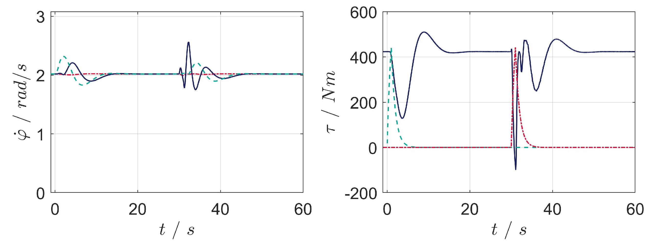
Figure 13.
Transient responses of the closed-loop system. Disturbance rejection: (solid blue), (dashed green) and (dash-dot red). Impulse torques are applied to the second mass at time s (dashed green) and to the first mass s (dash-dot red).
Figure 13.
Transient responses of the closed-loop system. Disturbance rejection: (solid blue), (dashed green) and (dash-dot red). Impulse torques are applied to the second mass at time s (dashed green) and to the first mass s (dash-dot red).

Figure 14.
Transient responses of the closed-loop system. Adaptation and angular velocity reference tracking in presence of the measurement noise: (solid blue), (dashed green), (dash-dot red) and r (dotted gray).
Figure 14.
Transient responses of the closed-loop system. Adaptation and angular velocity reference tracking in presence of the measurement noise: (solid blue), (dashed green), (dash-dot red) and r (dotted gray).

Figure 15.
Domain of parameters variation and simulation cases.

Figure 16.
Transient responses of the closed-loop system. Adaptation and angular velocity reference tracking in presence of parameter uncertainties: nominal parameter model (solid blue) and uncertain parameter model (dashed green).
Figure 16.
Transient responses of the closed-loop system. Adaptation and angular velocity reference tracking in presence of parameter uncertainties: nominal parameter model (solid blue) and uncertain parameter model (dashed green).


Table 1.
Model parameters.
| Name | Symbol | Value | Unit |
|---|---|---|---|
| Density of the motor shaft | 8000 | [kg/m] | |
| Shear modulus of the motor shaft | G | 79.3 | [N/m] |
| Structural damping of the motor shaft | [Nms] | ||
| Length of the motor shaft | L | 1500 | [m] |
| Moment of inertia of the motor shaft | I | [m] | |
| Moments of inertia of the first mass | 150 | [kg m] | |
| Moments of inertia of the second mass | 1500 | [kg m] | |
| Viscous friction on the first mass | 2000 | [Nms] | |
| Coulomb friction torque | 165 | [Nm] | |
| Viscous dissipation torque | 20 | [Nms] | |
| Static friction torque | 515 | [Nm] | |
| Stribeck parameter | [−] | ||
| Slope in the region of zero velocity | [−] |
Table 2.
Performance measures for .
| Cases | 1 | 2 | 3 | 4 | 5 | 6 | 7 | 8 | 9 |
|---|---|---|---|---|---|---|---|---|---|
| 9.27 | 8.22 | 10.46 | 9 | 12.25 | 9.92 | 9.80 | 8.68 | 11.15 | |
| 16.62 | 21.15 | 20.64 | 16.11 | 13.94 | 20.15 | 17.12 | 28.07 | 21.25 | |
| 8.97 | 4.32 | 15.08 | 5.53 | 2.04 | 12.01 | 12.96 | 9.48 | 18.52 |
Table 3.
Performance measures for .
| Cases | 1 | 2 | 3 | 4 | 5 | 6 | 7 | 8 | 9 |
|---|---|---|---|---|---|---|---|---|---|
| 7.44 | 6.40 | 8.62 | 7.26 | 10.46 | 8.12 | 7.91 | 6.71 | 9.28 | |
| 15 | 19.26 | 23.03 | 14.90 | 14.18 | 18.51 | 15.22 | 26.26 | 34.05 | |
| 12.74 | 5.38 | 22.79 | 7.44 | 1.92 | 18 | 19.03 | 11.57 | 28.19 |
Publisher’s Note: MDPI stays neutral with regard to jurisdictional claims in published maps and institutional affiliations. |
© 2021 by the authors. Licensee MDPI, Basel, Switzerland. This article is an open access article distributed under the terms and conditions of the Creative Commons Attribution (CC BY) license (https://creativecommons.org/licenses/by/4.0/).
Share and Cite
MDPI and ACS Style
Golovin, I.; Palis, S. PFC-Based Control of Friction-Induced Instabilities in Drive Systems. Machines 2021, 9, 134. https://0-doi-org.brum.beds.ac.uk/10.3390/machines9070134
AMA Style
Golovin I, Palis S. PFC-Based Control of Friction-Induced Instabilities in Drive Systems. Machines. 2021; 9(7):134. https://0-doi-org.brum.beds.ac.uk/10.3390/machines9070134
Chicago/Turabian StyleGolovin, Ievgen, and Stefan Palis. 2021. "PFC-Based Control of Friction-Induced Instabilities in Drive Systems" Machines 9, no. 7: 134. https://0-doi-org.brum.beds.ac.uk/10.3390/machines9070134
Note that from the first issue of 2016, this journal uses article numbers instead of page numbers. See further details here.