
Online Nonlinear Error Compensation Circuit Based on Neural Networks


1
Engineering Research Center for Navigation Technology, Department of Precision Instrument, Tsinghua University, Beijing 100084, China
2
Weapon and Control Department, Army Academy of Armored Forces, Beijing 100084, China
*
Author to whom correspondence should be addressed.
Machines 2021, 9(8), 151; https://0-doi-org.brum.beds.ac.uk/10.3390/machines9080151
Submission received: 17 June 2021
/
Revised: 22 July 2021
/
Accepted: 26 July 2021
/
Published: 31 July 2021
(This article belongs to the Section Micro/Nano Electromechanical Systems (MEMS/NEMS))
Abstract
:Nonlinear errors of sensor output signals are common in the field of inertial measurement and can be compensated with statistical models or machine learning models. Machine learning solutions with large computational complexity are generally offline or implemented on additional hardware platforms, which are difficult to meet the high integration requirements of microelectromechanical system inertial sensors. This paper explored the feasibility of an online compensation scheme based on neural networks. In the designed solution, a simplified small-scale network is used for modeling, and the peak-to-peak value and standard deviation of the error after compensation are reduced to 17.00% and 16.95%, respectively. Additionally, a compensation circuit is designed based on the simplified modeling scheme. The results show that the circuit compensation effect is consistent with the results of the algorithm experiment. Under SMIC 180 nm complementary metal-oxide semiconductor (CMOS) technology, the circuit has a maximum operating frequency of 96 MHz and an area of 0.19 mm2. When the sampling signal frequency is 800 kHz, the power consumption is only 1.12 mW. This circuit can be used as a component of the measurement and control system on chip (SoC), which meets real-time application scenarios with low power consumption requirements.
1. Introduction
Microelectromechanical system (MEMS) inertial sensors, such as gyroscopes, acceleration meters, angular position sensors (APS), are manufactured by the MEMS process. MEMS inertial sensors have the characteristics of small size, low cost, and low power consumption, and are widely used in the fields of aerospace, intelligent robots, vehicles, mobile equipment, etc. [1,2]. Compared with mechanical gyros or accelerometers, fiber gyros, laser gyros, APS under the printed circuit board (PCB) process, etc., the accuracy of MEMS inertial sensors needs to be further improved to expand the application field [3]. For accuracy improvement, the MEMS inertial sensors realization can be optimized from the structural design, MEMS process, signal processing circuit, error compensation scheme, and measurement and control algorithm. In terms of the error compensation scheme, the stability of output signal amplitude is an important indicator for the accuracy of inertial devices [4,5], which is affected by different kinds of error components.
Relevant works about MEMS inertial sensor measurement errors mainly focus on the deterministic error and nondeterministic error [6]. The deterministic error includes direct-current (DC) bias, misalignment, scale factor error, etc., which can be compensated by calibration [7]. The nondeterministic error, generated by mechanical noise, electrical noise, etc., includes complex nonlinear error components. This type of error directly affects the stability of the output signals and is difficult to be processed directly through device calibration [8]. Therefore, the modeling and compensation schemes of the nonlinear error components are widely studied and two mainstream research schemes [9,10,11,12,13,14,15,16,17,18,19,20,21,22,23,24,25,26] are formed, namely, (1) establishing a statistical model and performing error compensating and (2) error compensation schemes based on machine learning or deep learning.
Statistical methods can be used to analyze and suppress error components. The literature [9] reported the use of multilevel wavelet decomposition to process gyroscope and accelerometer measurement values, in which the high-frequency noise is removed. In the literature [10], Allan variance analysis is used to analyze and estimate the error component. The combined method of Allan variance analysis and wavelet threshold denoising algorithm is introduced in [11] to separate random drift and high-frequency white noise and establish an accurate error compensation model. Through power spectral density function analysis [12], the nondeterministic error can be modeled as Gaussian white noise or colored noise, and error compensated methods are analyzed [13]. In order to improve the accuracy of modeling, the empirical model decomposition [14], and autoregressive-moving-average (ARMA) time series model [15,16,17] are introduced into the error compensation schemes. Based on the Kalman filtering algorithm, the error compensation scheme can achieve better results and improve the accuracy of the statistical model [18,19].
The accuracy improvement of statistical methods requires accurate analysis and modeling of error components, while another research idea is to obtain model structure and model parameters with machine learning schemes. The researchers use multilayer perception machines [20,21], recurrent neural networks [22,23,24], mixed deep learning networks [25,26], etc. to establish error models. By training the collected data, the model parameters are calculated, and the error compensation results on the test dataset can have better accuracy improvement than statistical models. These methods obtain the network structure through the learned parameter values, reducing the requirements for accurate modeling. In practical applications, the trained model is used for error prediction, and error compensation of the output signal is performed. However, the complexity of calculations makes these solutions generally applied offline on platforms such as laptops, or on additional computing platforms such as digital signal processors (DSPs), which are inferior to the online compensation solutions of statistical models in terms of real-time performance.
The signal sampling frequency involved in the field of inertial measurement is generally tens to hundreds of kHz, and there are application requirements for low power consumption. Machine learning or deep learning solutions are easier to obtain high-precision models but have greater computational complexity and are difficult to meet the real-time application requirement. One solution is to analyze and design a simplified network model through model complexity analysis and optimization [24]. Another solution is to refer to artificial intelligence chips [27] widely used in neural network acceleration, performing circuit-level parallel processing solutions to solve real-time problems. Based on the above two points, the topic discussed in this article is the feasibility of an online nonlinear error circuit for MEMS inertial sensors based on neural networks. There are two issues analyzed in this paper, one is whether the simplest neural network, the multilayer perceptron (MLP), is sufficient for error model fitting; the other is whether the circuit-level implementation meets inertial measurement applications in terms of speed and power consumption.
The article is organized as follows: Section 2 discusses the problems to be solved and analyzes the feasibility and complexity of a nonlinear error compensation scheme based on the MLP algorithm. The design and simulation of digital circuits based on the implemented compensation algorithm are presented in Section 3. The performance evaluation is presented in Section 4. Finally, Section 5 provides conclusions and future research plans.
2. Problem Description and Introduction of Error Compensation Scheme
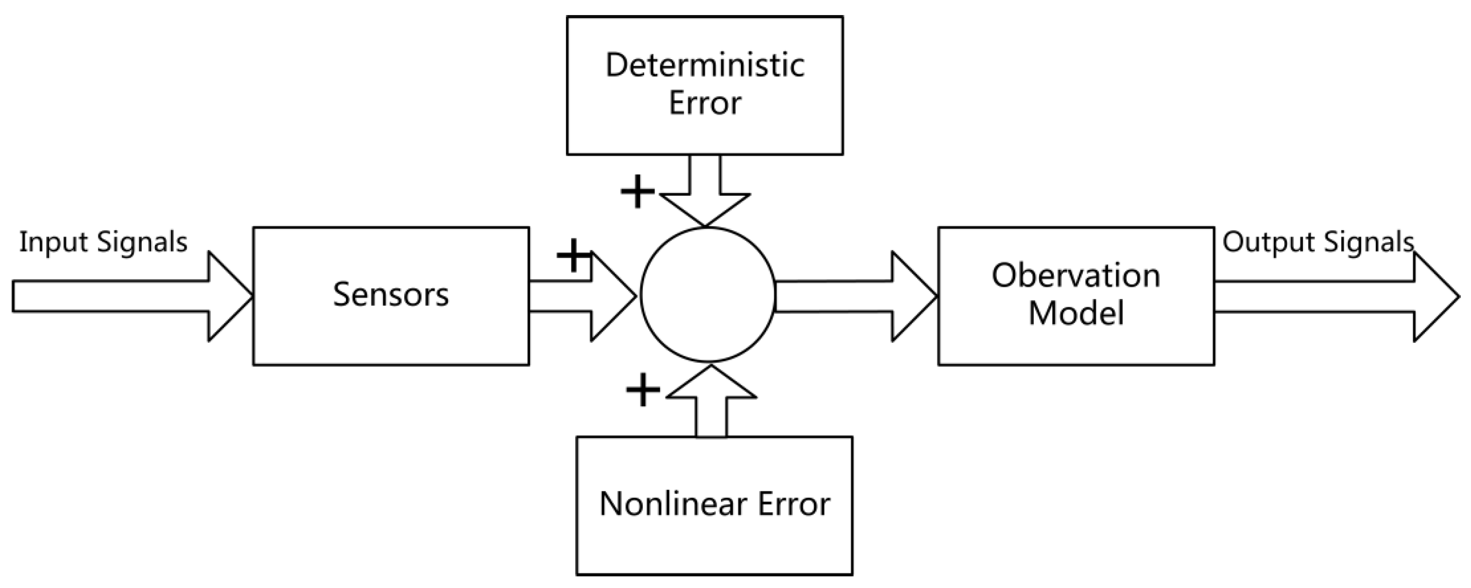
The output model of the MEMS inertial sensors is shown in Figure 1. After detecting the input signal, the sensor outputs the measurement signal according to the observation model. The output results are affected by deterministic factors and nonlinear errors. The deterministic factors include sensor deterministic error (bias, scale factor errors, etc.) and environmental error. The actual output model is as follows:
where represents the measurement output of the sensor, represents the true output of the sensor, represents the deterministic error of the sensor, represents the error caused by the environment, and represents the nonlinear error.
The nonlinear error in the composition of measurement error is discussed. In related research studies [9,10,11,12,13,14,15,16,17,18,19,20,21,22,23,24,25,26], the nonlinear error is modeled as a time series model, in which the error at the current moment is related to the observation values at previous moments. The error compensation scheme discussed in this paper is also based on the analysis of the time series model.
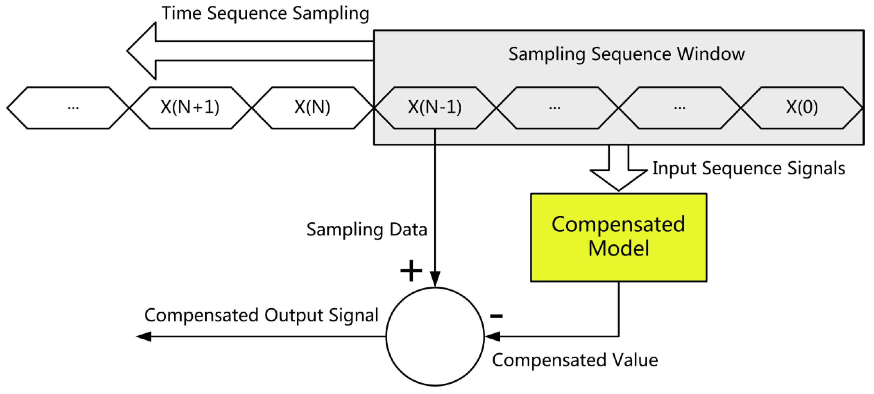
Figure 2 shows the schematic of the error compensation scheme. continuous data () are selected and preprocessed through the sliding window and sent to the compensation model, in which is the sampled value at the current moment, and the other data are the sampled value of previous moments. The compensation scheme uses the sampled data of the previous moments to compensate for the data of the current moment. The compensation model outputs the compensated value, and the output compensated signal of the current time is equal to the difference between and the compensation value.
The signal preprocessing process entails using the moving average filtering [24] to reduce the impact of white noise on the robustness of model fitting. The filtering process is as follows:
where represents one sample time, represents the length of the filtered sequence and represents the filtered data. The sampled data are filtered and sent to the compensation model to output the compensated value.
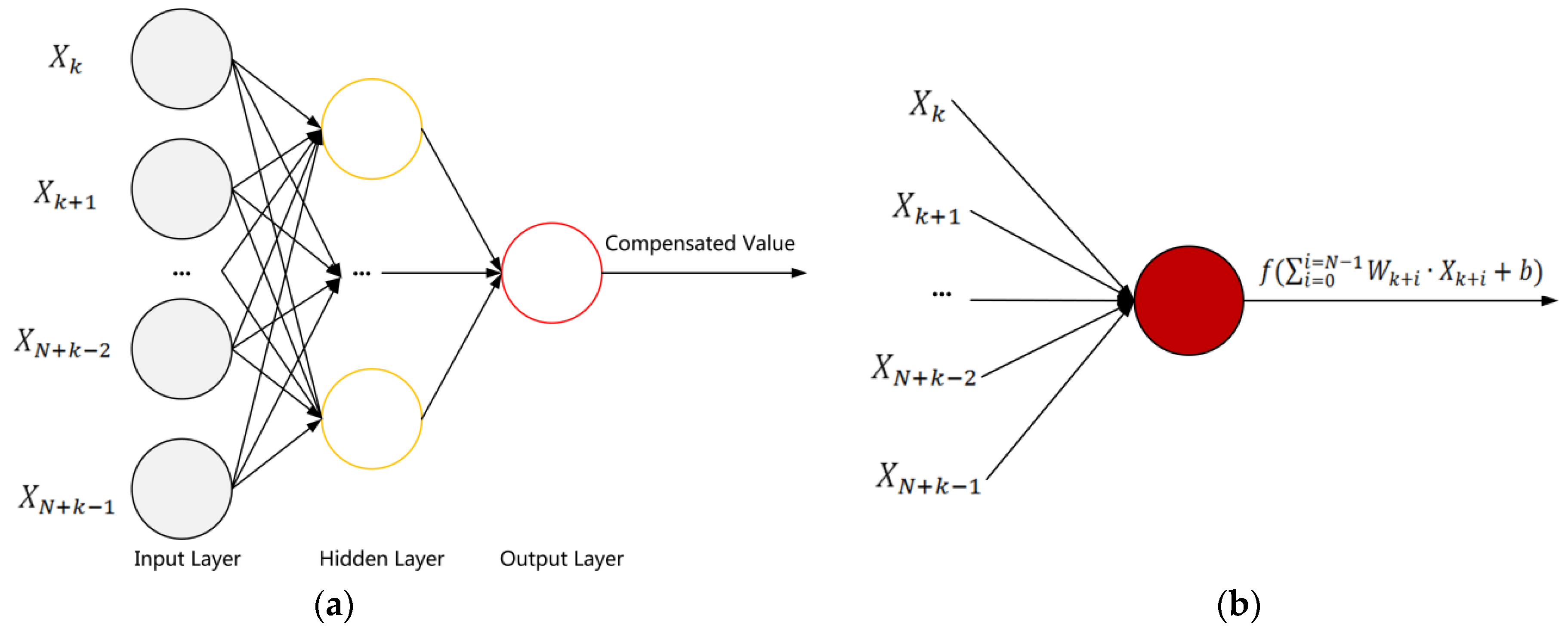
The compensation model used in the scheme is described in Figure 3. The compensated value is output through the MLP model, which is a simple neural network that includes an input layer, a hidden layer, and an output layer. The sampled continuous data are sent into the input layer, processed through the hidden layer with neuron model shown in Figure 3b, and then the compensation value is output. The output of a neuron can be expressed as , in which is the input vector, and are the weight and output bias to be trained and obtained, and is the activation function.
The key part of a neural network for nonlinear error fitting is the activation function, and the sigmoid activation function is commonly used in related works, which has the following expressions [20,21,22,23,24]:
where is the input value, and is the output activated value. The exponential calculation in the above function is complicated, and an activation function named leaky rectified linear units (ReLUs) [28] is used in the scheme to replace it. The expression is as follows:
where is a constant in the interval (1, ). This function is simple to be calculated and easy to be implemented at the circuit level.
3. Implementation Details and Experimental Results
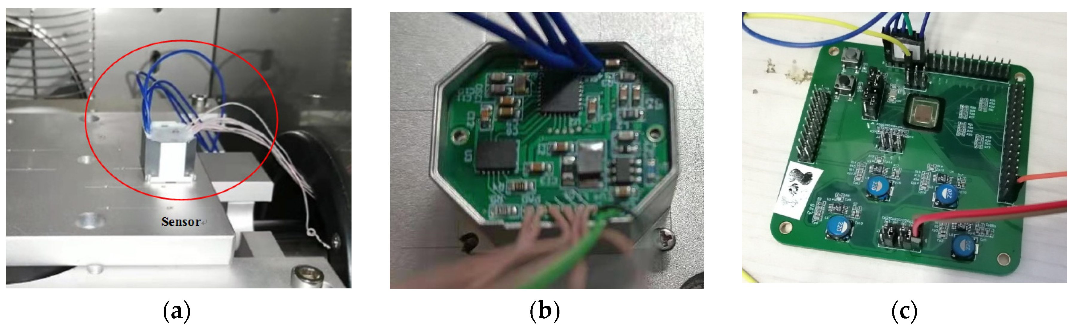
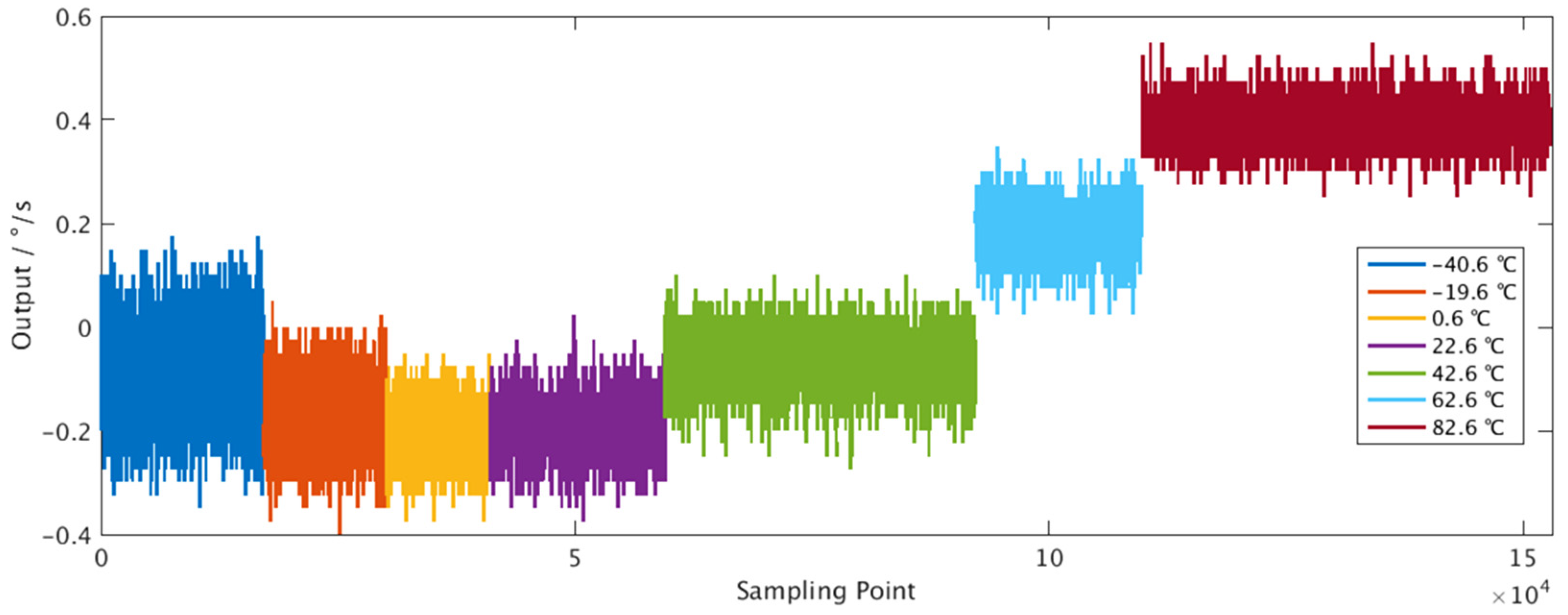
This section introduces the experimental results based on the above algorithm. The influence of network parameter scale and temperature on the results is also analyzed. As shown in Figure 4, the experimental device includes the inertial sensor ADIS16475 [29] and the data acquisition circuit [30]. The output data of the angular velocity under zero input in the X-axis direction of the sensor were collected and analyzed. Since the nonlinear error of the sensor is related to the temperature [31], the output data at a temperature of −40.6 °C, −19.6 °C, 0.6 °C, 22.6 °C, 42.6 °C, 62.6 °C, and 82.6 °C were collected in the experiment. A total of 152840 sets of data were analyzed, and the performance of the compensation scheme was analyzed at different temperatures.
The collected data are shown in Figure 5, which shows that temperature has an effect on the zero-bias output. The proposed solution works at a fixed temperature, while the error compensation effects at different temperatures are also carried out to show the solution effectiveness at different temperatures and the potential for error compensation in the full temperature range. The following analysis was carried out at a temperature of 22.6 °C, and the results were compared with related works. The data sets were divided into training sets and test sets in accordance with the proportion of 6:4. The first 60% of the collected data were used for training, and the remaining 40% of the data were used for scheme evaluation.
Before the data were further processed, the Kolmogorov–Smirnov (KS) test [32] was used to verify whether the training data and the test data set conform to the same distribution. After calculation, the p-value of the training data and the test data is 0.70, which is greater than 0.05, and the null hypothesis is not rejected. The results of the KS test show that it is reasonable to use neural network fitting models to suppress errors in short-term sampling data.
In the experiment, the window size of the moving average filter is a constant. Referring to Equation (2), is equal to 6. The MLP model was trained using the Adam optimizer [32]. The value of in Equation (4) is 5, and other parameters that need to be set include the number of neurons in the input layer and the hidden layer, which are defined as and , respectively. When and the signal output bias before and after compensation is shown in Table 1. From the experimental results, the peak-to-peak value and the standard deviation of the output bias are reduced by 17.00% and 16.95%, respectively, which reduce the fluctuation range of the output bias and improve the signal stability.
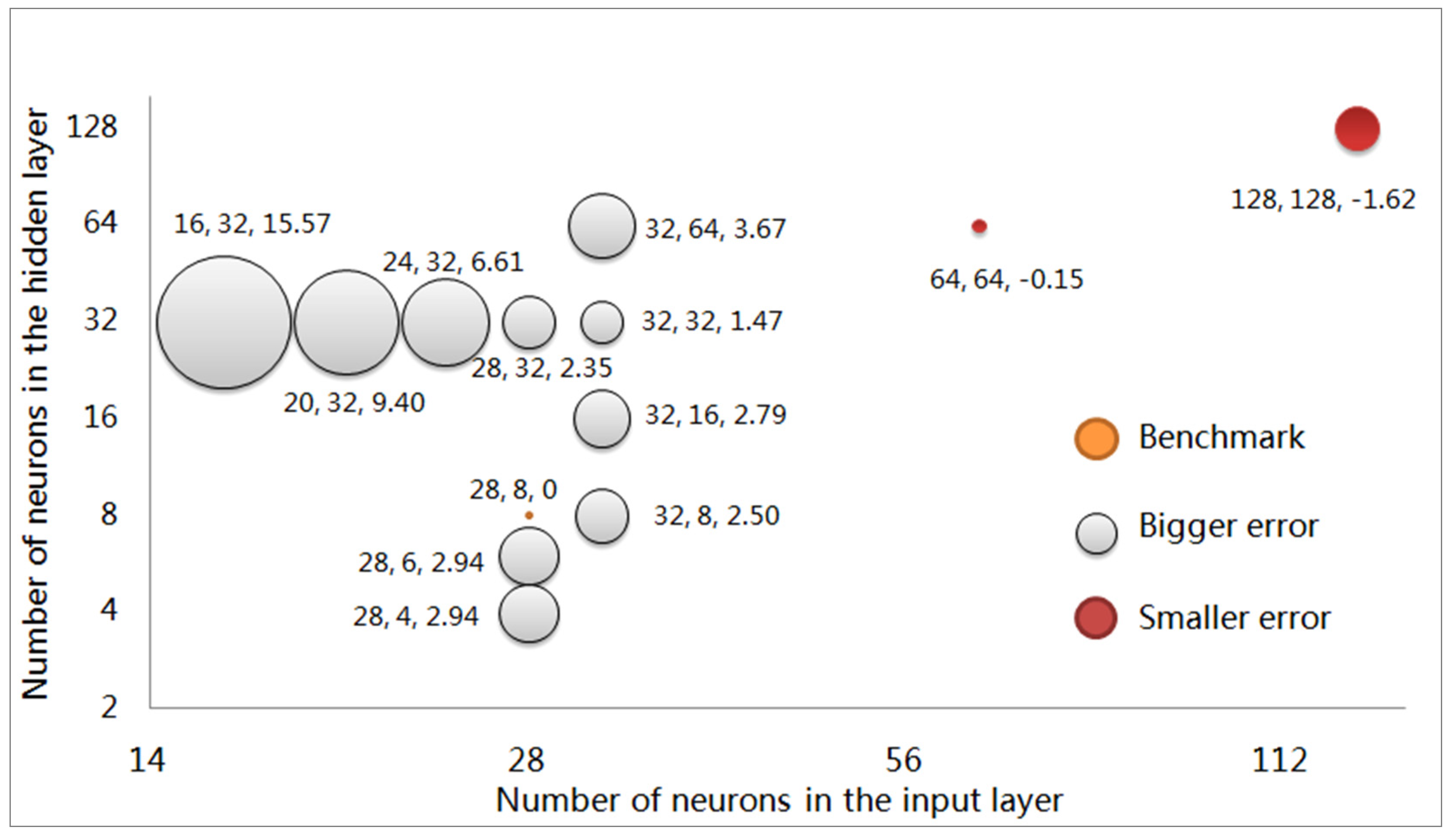
For the influence of the network parameter scale on the results, the parameter settings of the model were changed, and the error peak-to-peak value was used as an indicator to test the fitting effect. The compensated peak-to-peak value of and is taken as the comparison benchmark, and the increased ratio of the values, compared to the benchmark value under different parameters, is displayed in the bubble chart shown in Figure 6.
The yellow bubble in the figure represents the benchmark, red bubbles indicate that the error suppression effect is better than the benchmark, and the white bubbles indicate that the error suppression effect is worse than the benchmark. In Figure 6, there are three numbers next to the bubble, indicating the value of , and the peak-to-peak value growth percentage after error suppression compared to the benchmark.
The results shown in Figure 6 show that, compared with the selected benchmark value, when the parameter scale is enlarged, the proportion of further reduction of the error peak-to-peak value is limited. In the test process, a faster convergence speed of the model parameters occurs with larger values of and , while such a phenomenon does not exist when the values of and are greater than 128. For subsequent analysis and circuit design, and in the benchmark are set as network parameters.
In addition, the reduction ratios of error standard variance, compared with other machine-learning-based or deep-learning-based error suppression schemes are summarized in Table 2. The first column describes the various error suppression schemes, the second column lists the error suppression effects of the schemes, and the third column shows the performance improvement compared with the scheme adopted in this article. The percentage less than 100% indicates that the results presented in related works are better than the scheme adopted in this article, and the percentage greater than 100% indicates that the results are worse than the results of this article. Taking the scheme adopted in this article as a benchmark, for related works, a smaller percentage indicates better performance, while a greater percentage indicates worse performance.
All the related works in Table 2 are implemented offline. For real-time online signal processing, the results of the proposed scheme are compared with small-scale networks, and the use of MLP network and leaky ReLU activation function with simple calculations are sufficient to achieve the corresponding error suppression effect. From Table 2, when small-scale recurrent neural networks are used [23,24], the error suppression effect obtained is similar to that of the MLP network used in this article, and with large-scale networks [22,26], the error suppression effect obtained is better than that of the proposed method. The result of the comparison shows that the compensation effect of the adopted scheme at the algorithm level is effective and reasonable.
For the influence of the temperature on the results, the model fitting was performed on the data at different temperatures under the same network scale, and the error suppression effect was evaluated and summarized in Table 3. From the experimental results, the error suppression effect is similar at different temperatures. The discussed application scenario in this paper is the error suppression at a fixed temperature, and the error compensation model must be refitted at different temperatures. Taking the temperature as an input variable [31], the adopted method has the potential of error compensation in the full temperature range.
The experimental results in this section show that the adopted scheme has a simple calculation paradigm, and the compensation effect achieved under a small-scale network is even better than related works. The influence of different network scale parameters on the results is also analyzed and the network parameters with and are determined. The analysis of the compensation results at different temperatures shows that the scheme has the potential to suppress nonlinear errors in the full temperature range.
4. Circuit-Level Realization and Analysis of the Error Compensation Scheme
The computational complexity of the error compensation scheme based on neural networks is large, which is a challenge for real-time online applications. Compared with related works [22,23,24,25,26], the network model and activation function used in this paper are simpler and less complex. When the number of neurons in the input layer and the number of neurons in the hidden layer are and , the shape of the input vector is (1, ), the shape of the hidden layer parameter matrix is (, ), and the shape of the hidden layer feature matrix is (1,). Finally, a total of at least ) multiplication and addition operations, activation operations are required, which means at least machine cycles are required when the algorithm is running in the CPU. In the proposed design, and , and a low-power processor with a master clock frequency of 100 MHz is considered to implement the design, which can process at most 7.96 kHz sampling signals, which does not meet the requirements of tens to hundreds of kHz sampling signals required for inertial measurement.
Even for a simple network model adopted in this design, the above analysis illustrates the necessity of circuit-level implementation and acceleration of the algorithm. Circuit design and analysis based on the above scheme are presented in the following section.
4.1. Details of the Implemented Circuits
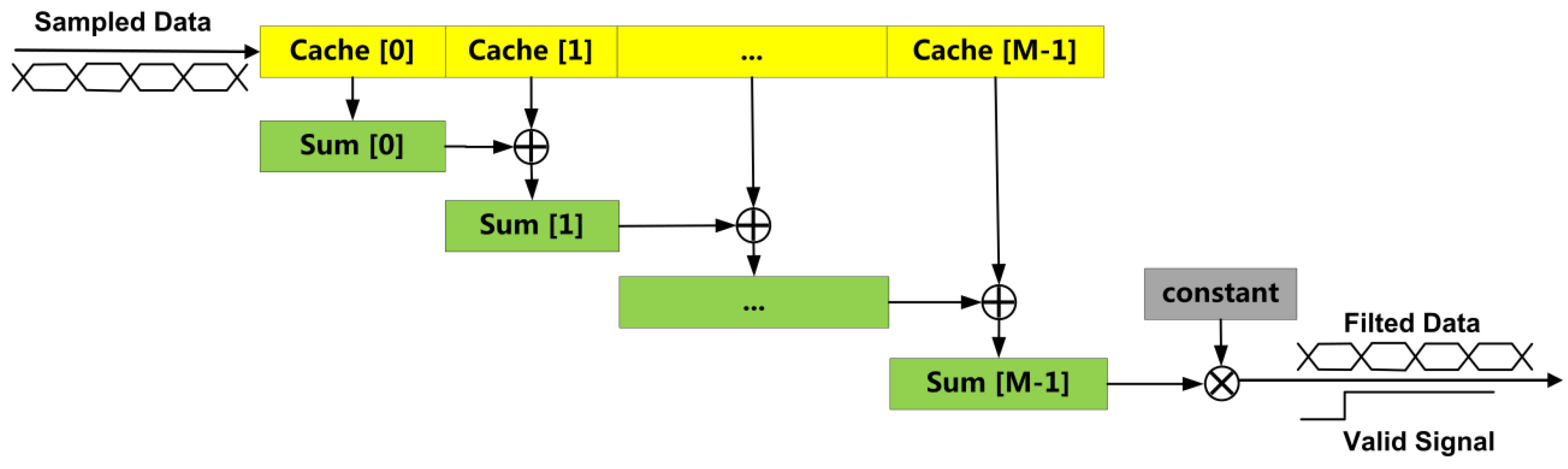
The collected signal from the sensor is 16-bit signed integers, which are expanded to 32 bits to reduce the effect of rounding errors in the calculation of fixed-point number multiplication. The sampled data are preprocessed by the moving average filtering circuit, and the implementation scheme is shown in Figure 7. The length of the filtered sequence is , and registers are contained in the circuit, in which the sampled data and the intermediate value of the summation calculation are cached, respectively. After the new data are sampled, the original cached data are stored at the next address, in turn, the last data no longer need to be stored, and the sampled data at this time are stored in the first position of the register array. The results of the summation calculation are updated at each sampling time.
The average operation after summation is a division by a constant, which is equivalent to the operation of multiplying by a constant. An -stage pipeline is adopted in the circuit, the signal is the output after a delay of clock cycles, and a valid signal is an output to indicate that the filtered signal is available. Finally, the filtered data with a valid signal will be updated with one clock cycle and be further processed by the MLP processing circuit.
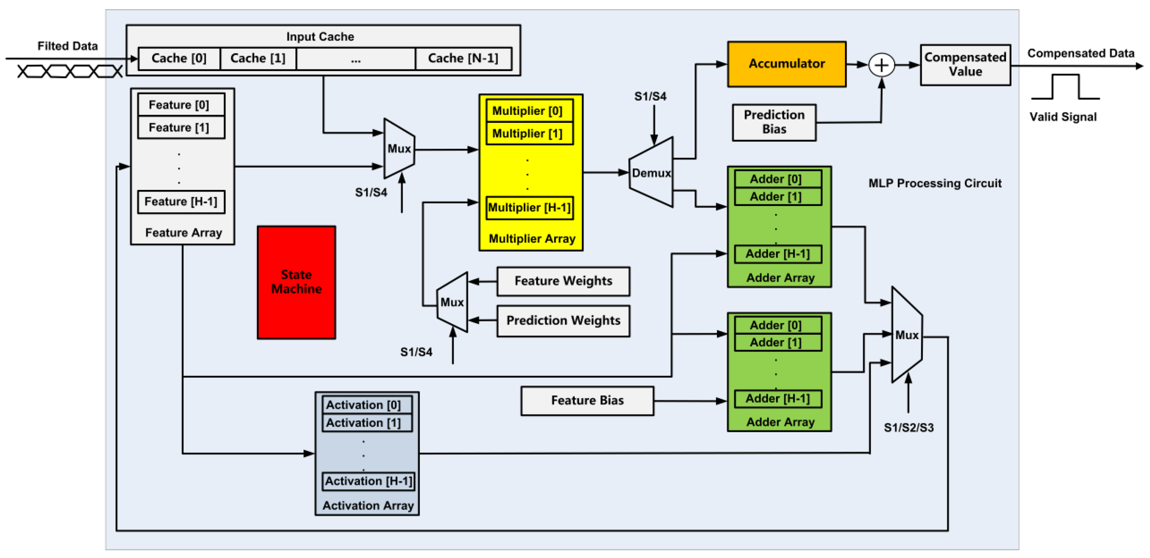
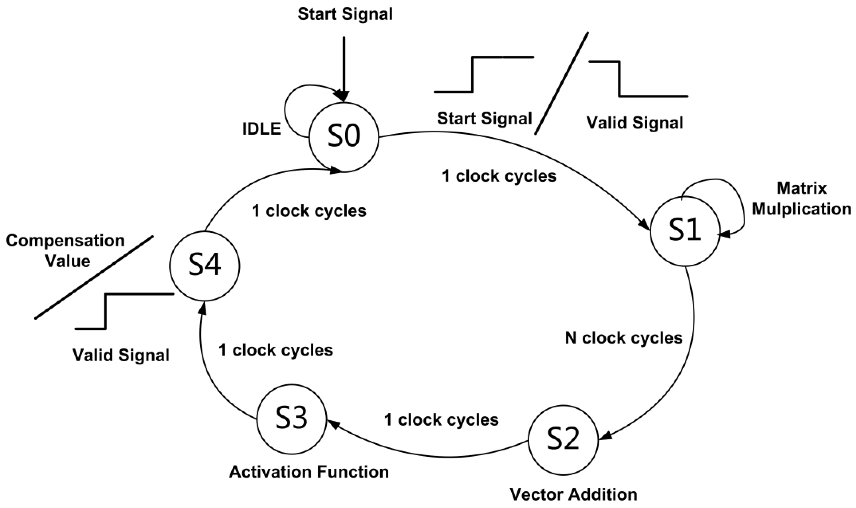
The data path and the control path of the MLP processing circuit are shown in Figure 8 and Figure 9, respectively. A finite state machine is used to process five states (S0, S1, S2, S3, and S4) in the calculation process. The cached data from the moving average filtering circuit are read in the S0 state, the matrix multiplication and the summation of the output bias of the hidden layer is performed in S1 and S2 states, respectively, the output activation of the hidden layer is performed in the S3 state, and the calculation of the compensation data of the output layer is performed in the S4 state. The multiplier array is multiplexed during hidden layer calculation and output calculation, and its input operands are selected by a multiplexer, and the selection signal is determined according to the current state from the finite state machine. The data of the feature matrix are updated through a multiplexer. The data derive from hidden layer matrix multiplication, bias addition, and activation function, and the selection signal is determined according to the current state.
multiplication operations, addition operations, and activation operations are required in the hidden layer, and the output layer requires multiplication operations and 1 addition operation. The most time-consuming operation is multiplication, and with multiple multipliers to process at the same time, the circuit processing time can be effectively reduced while the additional overhead of hardware resources is brought. In the circuit, multipliers are used to process calculations in the hidden layer neurons at the same time. The matrix multiplication of the hidden layer is completed in clock cycles, and the operation of the output layer is completed in one clock cycle.
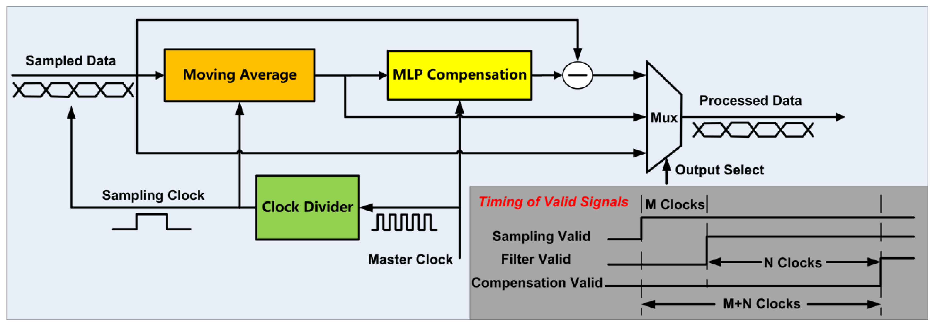
A start signal is needed to enable the MLP processing circuit. A total of + 4 clock cycles is needed to complete a compensation output, and a high-level effective valid signal is output when the compensated data are valid. The brief data path of the whole compensation circuit is shown in Figure 10. The continuous sampling signal passes through the moving average filter circuit and the MLP compensation circuit to obtain the compensation value, and the difference between the current sampling value and the compensation value is obtained as the compensated output data. The compensation circuit can select and output the uncompensated signal, the filtered signal, and the compensated signal through the multiplexer.
The frequency of the sampling clock and the master clock of the circuit are denoted by and , respectively. In order to streamline the compensation processing of the sampled data, the moving average circuit and MLP processing circuit need to complete data processing and data output in each sampling period. According to the above requirement, the required clock frequencies of the moving average filtering circuit and the MLP processing circuit are and , respectively. The following relationship between the sampling clock and the master clock is established:
The clock configuration relationship in Equation (4) enables the moving average filtering and MLP compensation to be completed once in each sampling clock cycle. The moving average filtering circuit has an output delay of , and the MLP circuit starts working when filtered data are cached, resulting in an output delay of . The output delay of the entire compensation circuit is . In the experiment, , , and , the number of multipliers consumed is 8, , and the output delay of the circuit is .
4.2. Analysis of the Implemented Results
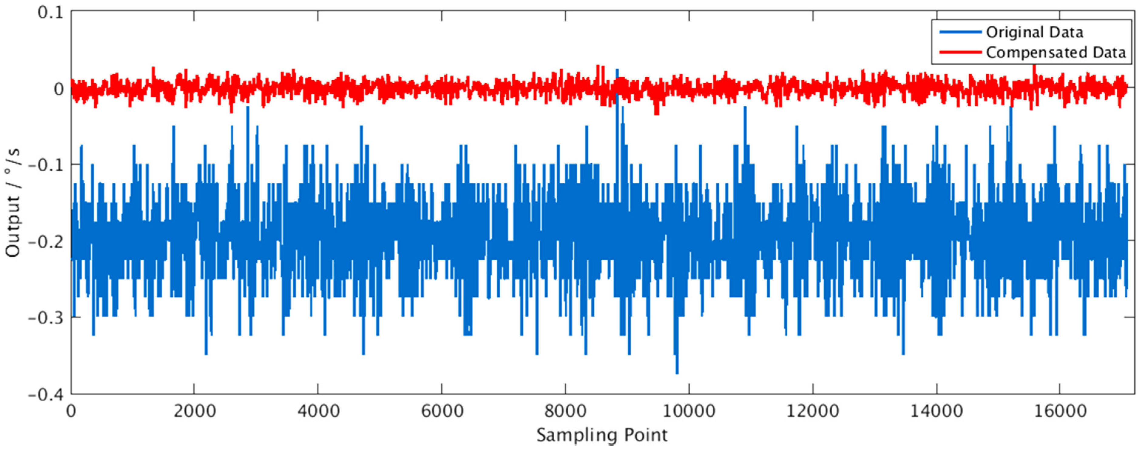
According to the design scheme of the compensation circuit, the Verilog hardware description language was used to realize the circuit, and the circuit-level error compensation experiment was carried out in VCS, a digital circuit analysis platform from Synopsys. The output data after compensation are 32-bit integers, multiplied by to obtain the real results, and were analyzed in MATLAB software. The signal waveforms before and after compensation are shown in Figure 11, and the signal information is shown in Table 4. The results of Table 1 and Table 4 are compared, indicating that the compensation of the circuit-level has no loss of precision.
The designed circuit is implemented and analyzed under the SMIC 180 nm complementary metal-oxide semiconductor (CMOS) process. Synthesis in Design Compiler and static timing analysis in Primetime were performed at three process corners—slow process (SS), typical process (TT), and fast process (FF). The maximum operating frequency of the system master clock is 96 MHz, corresponding to the sampling frequency of 3.2 MHz, which meets the requirements of inertial measurement.
Under the process corner TT (1.8 V voltage, 25 °C working temperature), when the frequency of the master clock is 96MHz and the sampling frequency is 3.2 MHz, the dynamic power consumption of the circuit obtained by Power Compiler is 4.22 mW. The dynamic power consumption of the circuit is positively related to the clock frequency. When the sampling signal is 800 kHz [2], the main clock frequency is 25.6 MHz, and the dynamic power consumption of the circuit is 1.12 mW, which meets the needs of low-power applications. In addition, the total cell area obtained from the area report is , in which the multiplier consumes more combinational area, which is a direction for resource optimization. The above analysis of power consumption and chip area is based on the results of digital front-end implementation. A more complete and accurate report needs to be obtained in conjunction with SoC and digital back-end implementation, and it is not discussed here.
5. Discussions and Conclusions
For the nonlinear error of the inertial sensors, a small-scale MLP network and the leaky ReLU activation function with simple calculations were used for error suppression, in which the error peak-to-peak value and standard variance are reduced to 17.00% and 16.95%, respectively. The experimental results confirm the effectiveness of the adopted scheme in the short-term, constant temperature working condition. For the real-time, online, and low-power requirements of edge devices, a digital processing circuit based on the developed method was designed, and the error suppression effect of the compensation circuit is consistent with the results in the algorithm verification experiments. For the circuit performance evaluation results, the supported maximum signal sampling frequency is 3.2 MHz, and the area of the circuit under the SMIC 180 process is . When the frequency of the master clock is 25.6 MHz, the total power consumption is only 1.12 mW, which meets the demand for low-power application scenarios. Circuit-level design and experiments confirm the feasibility of the on-chip solution for real-time and online applications.
In the experiment, the compensation effects with networks of the same parameter scale under different temperatures were analyzed. Although the compensation schemes still have similar error suppression effects, the trained parameters have different values and the assumed working condition should be a constant temperature. Temperature compensation of nonlinear error should be studied and processed in future research. In addition, the output signals of inertial sensors are affected by bias drift after working for a long time, and the statistical characteristics and distribution functions of the error may also change, which brings challenges to the robustness of the machine learning series of error compensation solutions. In terms of circuit design, the multiple frequency processing clock of the MLP compensation circuit limits the increase in the maximum sampling frequency. In addition to providing more on-chip computing resources, the optimization of the circuit data path and control path is also worth exploring.
In the collected experimental data, the working temperature has a major influence on the zero offsets. For future research, temperature information should be considered for compensation of nonlinear errors, and the coprocessor circuit of the compensation scheme will be integrated with the SoC to realize sensor drive, demodulation, and compensation of detected signals on a single processing chip.
Author Contributions
Conceptualization, R.Z. and B.Z.; methodology, Q.W.; software, C.J.; validation, X.Z. and Z.G.; formal analysis, Z.G.; investigation, Z.G.; resources, R.Z.; data curation, Z.G.; writing—original draft preparation, Z.G.; writing—review and editing, B.Z., Q.W. and C.J.; visualization, X.Z.; supervision, R.Z.; project administration, B.Z. and Q.W.; funding acquisition, B.Z. and Q.W. All authors have read and agreed to the published version of the manuscript.
Funding
This project is supported by the National Key R&D Program of China under (grant No.2018YFB1702500).
Institutional Review Board Statement
Not applicable.
Informed Consent Statement
Not applicable.
Data Availability Statement
Data sharing is not applicable.
Conflicts of Interest
The authors declare no conflict of interest.
References
- Tamazin, M.; Noureldin, A.; Korenberg, M. Nonlinear modeling of the stochastic errors of MEMS inertial sensors utilized in smart phones. In Proceedings of the 2013 1st International Conference on Communications, Signal Processing, and Their Applications (ICCSPA), Sharjah, United Arab Emirates, 12–14 February 2013. [Google Scholar]
- Gao, Z.; Zhou, B.; Li, X.; Yang, L.; Wei, Q.; Zhang, R. A Digital-Analog Hybrid System-on-Chip for Capacitive Sensor Measurement and Control. Sensors 2021, 21, 431. [Google Scholar] [CrossRef] [PubMed]
- Han, S.; Meng, Z.; Omisore, O.; Akinyemi, T.; Yan, Y. Random Error Reduction Algorithms for MEMS Inertial Sensor Accuracy Improvement. Micromachines 2020, 11, 1021. [Google Scholar] [CrossRef] [PubMed]
- Bhardwaj, R. Errors in micro-electro-mechanical systems inertial measurement and a review on present practices of error modelling. Trans. Inst. Meas. Control. 2018, 40, 2843–2854. [Google Scholar] [CrossRef]
- Tang, P.; Tan, T.; Trinh, C. Characterizing Stochastic Errors of MEMS—Based Inertial Sensors. VNU J. Sci. Math. Phys. 2016, 32, 34–42. [Google Scholar]
- Radi, A.; Sheta, B.; Nassar, S.; Arafa, I.; Youssef, A.; El-Sheimy, N. Accurate Identification and Implementation of Complicated Stochastic Error Models for Low-Cost MEMS Inertial Sensors. In Proceedings of the 2020 12th International Conference on Electrical Engineering (ICEENG), Cairo, Egypt, 7–9 July 2020. [Google Scholar]
- Lin, X.; Zhang, X. Random Error Compensation of MEMS Gyroscope Based on Adaptive Kalman Filter. In Proceedings of the 2020 Chinese Control and Decision Conference (CCDC), Hefei, China, 22–24 August 2020; pp. 1206–1210. [Google Scholar]
- Bai, Y.; Wang, X.; Jin, X.; Su, T.; Kong, J.; Zhang, B. Adaptive filtering for MEMS gyroscope with dynamic noise model. ISA Trans. 2020, 101, 430–441. [Google Scholar] [CrossRef]
- El-Sheimy, N.; Nassar, S.; Noureldin, A. Wavelet de-noising for IMU alignment. IEEE Aerosp. Electron. Syst. Mag. 2004, 19, 32–39. [Google Scholar] [CrossRef]
- Vaccaro, R.J.; Zaki, A.S. Statistical Modeling of Rate Gyros. IEEE Trans. Instrum. Meas. 2012, 61, 673–681. [Google Scholar] [CrossRef]
- Zhang, R.; Gao, S.; Cai, X. Modeling of MEMS gyro drift based on wavelet threshold denoising and improved Elman neural network. In Proceedings of the 2019 14th IEEE International Conference on Electronic Measurement & Instruments (ICEMI), Changsha, China, 1–3 November 2019. [Google Scholar]
- Han, S.; Wang, J. Quantization and Colored Noises Error Modeling for Inertial Sensors for GPS/INS Integration. IEEE Sens. J. 2010, 11, 1493–1503. [Google Scholar] [CrossRef]
- Lv, P.; Lai, J.; Liu, J.; Nie, M. The Compensation Effects of Gyros’ Stochastic Errors in a Rotational Inertial Navigation System. J. Navig. 2014, 67, 1069–1088. [Google Scholar] [CrossRef]
- Xu, G.; Tian, W.; Qian, L. EMD- and SVM-based temperature drift modeling and compensation for a dynamically tuned gyroscope (DTG). Mech. Syst. Signal Process. 2007, 21, 3182–3188. [Google Scholar] [CrossRef]
- Wang, K.; Wu, Y.; Gao, Y.; Li, Y. New methods to estimate the observed noise variance for an ARMA model. Measurement 2017, 99, 164–170. [Google Scholar] [CrossRef]
- Song, J.; Shi, Z.; Wang, L.; Wang, H. Improved Virtual Gyroscope Technology Based on the ARMA Model. Micromachines 2018, 9, 348. [Google Scholar] [CrossRef] [PubMed] [Green Version]
- Li, L. Random Error Recognition and Noise Reduction Technology of MEMS Gyro. In Proceedings of the 2019 International Conference on Artificial Intelligence and Computer Science, Xalapa, Mexico, 27 October–2 November 2019; pp. 713–716. [Google Scholar] [CrossRef]
- Narasimhappa, M.; Nayak, J.; Terra, M.H.; Sabat, S.L. ARMA model based adaptive unscented fading Kalman filter for reducing drift of fiber optic gyroscope. Sens. Actuators A Phys. 2016, 251, 42–51. [Google Scholar] [CrossRef]
- Xue, L.; Jiang, C.; Wang, L.; Liu, J.; Yuan, W. Noise Reduction of MEMS Gyroscope Based on Direct Modeling for an Angular Rate Signal. Micromachines 2015, 6, 266–280. [Google Scholar] [CrossRef]
- Xia, D.; Chen, S.; Wang, S.; Li, H. Microgyroscope Temperature Effects and Compensation-Control Methods. Sensors 2009, 9, 8349–8376. [Google Scholar] [CrossRef]
- Zhang, R.; Xu, B.; Shi, P. Output Feedback Control of Micromechanical Gyroscopes Using Neural Networks and Disturbance Observer. IEEE Trans. Neural Netw. Learn. Syst. 2020. [Google Scholar] [CrossRef]
- Jiang, C.; Chen, S.; Chen, Y.; Bo, Y.; Han, L.; Guo, J.; Feng, Z.; Zhou, H. Performance Analysis of a Deep Simple Recurrent Unit Recurrent Neural Network (SRU-RNN) in MEMS Gyroscope De-Noising. Sensors 2018, 18, 4471. [Google Scholar] [CrossRef] [PubMed] [Green Version]
- Zhu, C.; Cai, S.; Yang, Y.; Xu, W.; Shen, H.; Chu, H. A Combined Method for MEMS Gyroscope Error Compensation Using a Long Short-Term Memory Network and Kalman Filter in Random Vibration Environments. Sensors 2021, 21, 1181. [Google Scholar] [CrossRef]
- Li, D.; Zhou, J.; Liu, Y. Recurrent-neural-network-based unscented Kalman filter for estimating and compensating the random drift of MEMS gyroscopes in real time—ScienceDirect. Mech. Syst. Signal Process. 2021, 147, 107057. [Google Scholar] [CrossRef]
- Jiang, C.; Chen, Y.; Chen, S.; Bo, Y.; Li, W.; Tian, W.; Guo, J. A Mixed Deep Recurrent Neural Network for MEMS Gyroscope Noise Suppressing. Electronics 2019, 8, 181. [Google Scholar] [CrossRef] [Green Version]
- Han, S.; Meng, Z.; Zhang, X.; Yan, Y. Hybrid Deep Recurrent Neural Networks for Noise Reduction of MEMS-IMU with Static and Dynamic Conditions. Micromachines 2021, 12, 214. [Google Scholar] [CrossRef] [PubMed]
- Latotzke, C.; Gemmeke, T. Efficiency Versus Accuracy: A Review of Design Techniques for DNN Hardware Accelerators. IEEE Access 2021, 9, 9785–9799. [Google Scholar] [CrossRef]
- Lee, J.-H.; Marzelli, M.; Jolesz, F.A.; Yoo, S.-S. Automated classification of fMRI data employing trial-based imagery tasks. Med. Image Anal. 2009, 13, 392–404. [Google Scholar] [CrossRef] [Green Version]
- ADIS16475. Available online: https://www.analog.com/media/en/technical-documentation/data-sheets/ADIS16475.pdf (accessed on 5 November 2019).
- Gao, Z.; Zhou, B.; Li, Y.; Yang, L.; Li, X.; Wei, Q.; Chu, H.; Zhang, R. Design and Implementation of an On-Chip Low-Power and High-Flexibility System for Data Acquisition and Processing of an Inertial Measurement Unit. Sensors 2020, 20, 462. [Google Scholar] [CrossRef] [PubMed] [Green Version]
- El-Diasty, M.; Pagiatakis, S. A Rigorous Temperature-Dependent Stochastic Modelling and Testing for MEMS-Based Inertial Sensor Errors. Sensors 2009, 9, 8473. [Google Scholar] [CrossRef] [PubMed] [Green Version]
- Berger, V.W.; Zhou, Y.Y. Kolmogorov–Smirnov Test: Overview; John Wiley & Sons, Ltd.: Hoboken, NJ, USA, 2014. [Google Scholar]
Figure 1.
Measurement model of a MEMS inertial sensor.

Figure 2.
Schematic of the error compensation scheme.

Figure 3.
Output model of compensated value based on MLP: (a) structure of the output model; (b) mathematical model of a neuron in MLP.
Figure 3.
Output model of compensated value based on MLP: (a) structure of the output model; (b) mathematical model of a neuron in MLP.

Figure 4.
Experimental equipment for data collection: (a) the sensor in a thermostat; (b) signal preprocessing circuit; (c) circuit for digital signal acquisition and output.
Figure 4.
Experimental equipment for data collection: (a) the sensor in a thermostat; (b) signal preprocessing circuit; (c) circuit for digital signal acquisition and output.

Figure 5.
The collected output bias data at different temperatures.

Figure 6.
Error compensation effect under different parameter scales.

Figure 7.
The data path of the moving average filtering circuit.

Figure 8.
The data path of the MLP processing circuit.

Figure 9.
Description of the state machine in MLP processing circuit.

Figure 10.
The brief data path of the compensation circuit.

Figure 11.
Signal waveforms of original data and compensated data.


Table 1.
Summary of signal output bias before and after compensation.
| Category | Standard Deviation | Maximum Value | Minimum Value | Average Value | Peak-to-Peak Value |
|---|---|---|---|---|---|
| Before compensation | 0.059 °/s | 0.025 °/s | −0.375 °/s | −0.193 °/s | 0.400 °/s |
| After compensation | 0.010 °/s | 0.031 °/s | −0.037 °/s | −0.001 °/s | 0.068 °/s |
| Ratio | 16.95% | 124.00% | 9.87% | 0.52% | 17.00% |
Table 2.
Comparison of different error suppression solutions.
| Category | Reduction Ratio of Standard Deviation | Percentage |
|---|---|---|
| Adopted method | 16.95% | / |
| SRU-RNN [22] | 12.5% | 73.75% |
| BiLSTM [23] | 53.19% | 313.81% |
| BiLSTM-ARMA-KF [23] | 48.17% | 284.19% |
| BiLSTM-EM-KF [23] | 25.75% | 151.92% |
| RNN-based UKF [24] | 32.77% | 193.33% |
| LSTM-LSTM [26] | 4.05% | 23.89% |
| GRU-GRU [26] | 2.47% | 14.57% |
| LSTM-GRU [26] | 2.21% | 13.04% |
| GRU-LSTM [26] | 1.61% | 9.50% |
Table 3.
Error compensated effect under different temperatures.
| Temperature | Original Peak-to-Peak Value | Compensated Peak-to-Peak Value | Ratio |
|---|---|---|---|
| −40.6 °C | 0.525 °/s | 0.104 °/s | 19.81% |
| −19.6 °C | 0.450 °/s | 0.082 °/s | 18.22% |
| 0.6 °C | 0.325 °/s | 0.058 °/s | 17.85% |
| 22.6 °C | 0.400 °/s | 0.068 °/s | 17.00% |
| 42.6 °C | 0.375 °/s | 0.068 °/s | 18.13% |
| 62.6 °C | 0.325 °/s | 0.059 °/s | 18.15% |
| 82.6 °C | 0.300 °/s | 0.048 °/s | 16.00% |
Table 4.
Summary of signal information before and after circuit compensation.
| Category | Standard Deviation | Maximum Value | Minimum Value | Average Value | Peak-to-Peak Value |
|---|---|---|---|---|---|
| Before compensation | 0.059 °/s | 0.025 °/s | −0.375 °/s | −0.193 °/s | 0.400 °/s |
| Circuit compensation | 0.010 °/s | 0.031 °/s | −0.036 °/s | −0.001 °/s | 0.068 °/s |
| Ratio (Circuit) | 16.95% | 124.00% | 9.60% | 0.52% | 17.00% |
| Ratio (CPU) | 16.95% | 124.00% | 9.87% | 0.52% | 17.00% |
Publisher’s Note: MDPI stays neutral with regard to jurisdictional claims in published maps and institutional affiliations. |
© 2021 by the authors. Licensee MDPI, Basel, Switzerland. This article is an open access article distributed under the terms and conditions of the Creative Commons Attribution (CC BY) license (https://creativecommons.org/licenses/by/4.0/).
Share and Cite
MDPI and ACS Style
Gao, Z.; Zhou, B.; Ju, C.; Wei, Q.; Zhang, X.; Zhang, R. Online Nonlinear Error Compensation Circuit Based on Neural Networks. Machines 2021, 9, 151. https://0-doi-org.brum.beds.ac.uk/10.3390/machines9080151
AMA Style
Gao Z, Zhou B, Ju C, Wei Q, Zhang X, Zhang R. Online Nonlinear Error Compensation Circuit Based on Neural Networks. Machines. 2021; 9(8):151. https://0-doi-org.brum.beds.ac.uk/10.3390/machines9080151
Chicago/Turabian StyleGao, Zhenyi, Bin Zhou, Chunge Ju, Qi Wei, Xinxi Zhang, and Rong Zhang. 2021. "Online Nonlinear Error Compensation Circuit Based on Neural Networks" Machines 9, no. 8: 151. https://0-doi-org.brum.beds.ac.uk/10.3390/machines9080151
Note that from the first issue of 2016, this journal uses article numbers instead of page numbers. See further details here.