Synchronization Control of a Dual-Cylinder Lifting Gantry of Segment Erector in Shield Tunneling Machine under Unbalance Loads

Abstract

Segment assembling is one of the principle processes during tunnel construction using shield tunneling machines. The segment erector is a robotic manipulator powered by a hydraulic system to assemble prefabricated concrete segments onto the excavated tunnel surface. Nowadays, automation of the segment erector has become one of the definite developing trends to further improve the efficiency and safety during construction; thus, closed-loop motion control is an essential technology. Within the segment erector, the lifting gantry is driven by dual cylinders to lift heavy segments in the radial direction. Different from the dual-cylinder mechanism used in other machines such as forklifts, the lifting gantry usually works at an inclined angle, leading to unbalanced loads on the two sides. Although strong guide rails are applied to ensure synchronization, the gantry still occasionally suffers from chattering, “pull-and-drag”, or even being stuck in practice. Therefore, precise motion tracking control as well as high-level synchronization of the dual cylinders have become essential for the lifting gantry. In this study, a complete dynamics model of the dual-cylinder lifting gantry is constructed, considering the linear motion as well as the additional rotational motion of the crossbeam, which reveals the essence of poor synchronization. Then, a two-level synchronization control scheme is synthesized. The thrust allocation is designed to coordinate the dual cylinders and keep the rotational angle of the crossbeam within a small range. The motion tracking controller is designed based on the adaptive robust control theory to guarantee the linear motion tracking precision. The theoretical performance is analyzed with corresponding proof. Finally, comparative simulations are conducted and the results show that the proposed scheme achieves high-precision motion tracking performance and simultaneous high-level synchronization of dual cylinders under unbalanced loads.

1. Introduction

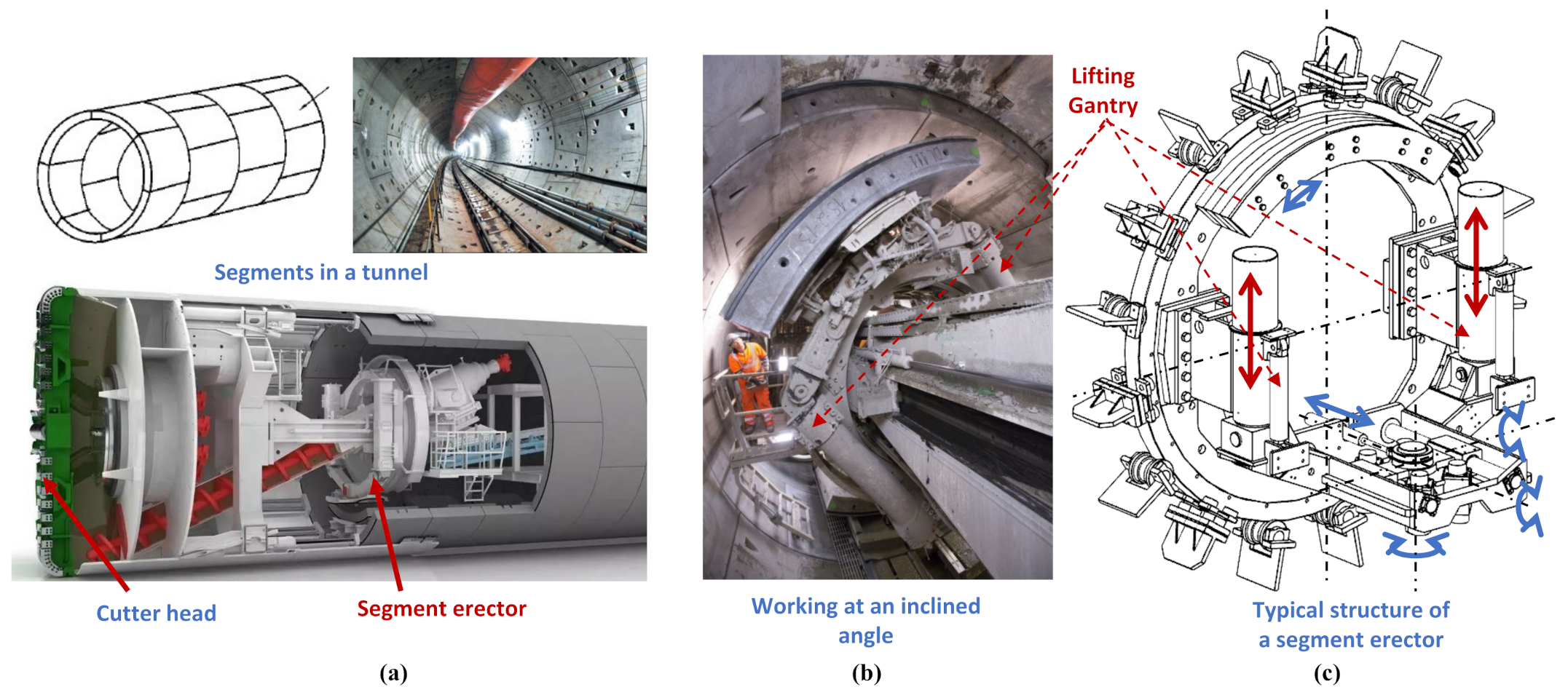
A shield tunneling machine is widely used for excavating tunnels in soft ground [1]. During tunnel construction, there are two main processes that take place in turn, i.e., shield tunneling and segment assembling. The former is the core process beyond all doubt, while the latter is also extremely essential for the quality, efficiency, and safety of the entire construction. General structures of a tunnel and a shield tunneling machine are shown in Figure 1a. As the figure shows, the cutter head rotates to excavate the tunnel, and then the prefabricated concrete segments are assembled onto the excavated surface to form a permanent support for the tunnel. The robotic manipulator for the segment assembling process is called the “segment erector”, and Figure 1b shows a real one working in a practical shield tunneling machine. The segment erector needs to be very precise in handling heavy segments, which can be up to several tons depending on the diameter of the tunnel. A typical structure of the segment erector is given Figure 1c. It offers complete handling of the segment with six degrees-of-freedom (6 DOFs), including lifting in the radial direction, sliding in the axial direction, and rotating around the central axis of the shield tunnel machine, and 3 DOFs of rolling, pitching, and yawing in the clamping head [2]. Although, nowadays, almost all of the segment erectors used in construction are human-operated, automation has become one of the definite developing trends to further improve the efficiency and safety in tunnel construction. Recently, much attention has been paid to the automation of the entire shield tunneling machine [3,4,5] as well as the segment assembling [6,7,8]. To the best of our knowledge, all segment erectors are driven by hydraulic systems because of the large power-to-weight ratio [9,10,11,12,13]. In order to achieve automation, closed-loop motion control of the segment erector is one of the fundamental technologies.

Within a typical segment erector, the lifting gantry, which is the focus in this study, is driven by dual cylinders to generate the required large lifting force and ensure the stability of the motion. Thus, high-level motion synchronization of the dual cylinders becomes essential. However, as shown in Figure 1b,c, different from the dual-cylinder mechanism used in other machines, such as forklifts [14,15], the lifting gantry usually works at an inclined angle, which leads to unbalanced loads on the two sides. Since the segment is very heavy and the crossbeam of the gantry is up to 3 m to 7 m long depending on the diameter of the tunnel, the forces on the dual cylinders can vary widely, making motion synchronization more challenging. Although strong guide rails are applied in the lifting gantry to ensure synchronization, the gantry still occasionally suffers from chattering, “pull-and-drag”, or even being stuck in practice due to poor synchronization under largely unbalanced loads. Therefore, a motion synchronization control scheme for the lifting gantry under unbalanced loads is the basis of high-precision closed-loop control of the segment erector.

In fact, there have been a large number of studies concerning the synchronization control of dual actuators, such as the linear motor gantry [16,17], dual motors in vehicles [18], and redundant hydraulic cylinders in airplanes [19]. Since the dynamics of hydraulic systems are highly nonlinear, with inherent nonlinearities and uncertainties [20,21], high-level synchronization control of hydraulic cylinders is more challenging compared with other actuators [22,23]. As for the control schemes, early ones have applied the same control signals for the dual cylinders. Apparently, if the gantry is vertical or horizontal, with balanced loads for dual sides, such a scheme is able to achieve reasonable precision with some mechanical couplings to guarantee motion synchronization. However, if the loads become largely unbalanced, the synchronization performance can only depend on the mechanical couplings arbitrarily, without any efforts made by the controller. Essentially, such an intuitive scheme shares no information between the dual cylinders, e.g., the motion discrepancies, which possibly leads to poor synchronization in practice [16]. Another common scheme is cross-coupled control [24], which is based on the idea of contouring control for a multi-axis system. In this scheme, a synchronization compensator is constructed according to the kinetics information between the two cylinders, such as the relative position and velocity, leading to better synchronization performance under different drive characteristics and loading conditions of the individual cylinders [25]. However, this scheme still tries to solve the motion synchronization problem from the kinetics level, and ignores the influence of the mechanical coupling, which will possibly lead to additional internal forces and performance degradation [16].

Essentially, the existence of poor synchronization in the presence of the strong mechanical coupling between the dual cylinders in the lifting gantry implies that there is a component that is not rigid enough. In other words, in addition to the principle linear motion, the gantry must allow a rotational motion to some extent, which explains the essence of poor synchronization as the rotation of the crossbeam. For example, both [16] and [26] have performed the modeling of a linear dual-drive gantry with consideration of the rotational motion and synthesized model-based controllers to deal with the additional degree-of-freedom. Thus, in order to achieve high-precision control of the lifting gantry under unbalanced loads, a complete model including both linear and rotational motions should be constructed. In addition, the large mass and rotational inertia of the segment as well as the mechanical coupling with high stiffness should be considered in building the dynamics model. However, to the best of our knowledge, there have been few studies proposing such a complete model of the dual-cylinder lifting gantry working at an inclined angle.

Poor synchronization of the dual cylinders will cause the crossbeam to rotate and then result in excessive internal forces produced by the mechanical coupling. Moreover, consequent chattering and “pull-and-drag” phenomena are adverse to the stability and precision of the entire segment erector. Therefore, in this study, a model-based synchronization control scheme is proposed, for high-precision motion tracking performance of the dual-cylinder lifting gantry of the segment erector under unbalanced loads. To guarantee the tracking performance in the presence of various nonlinearities and uncertainties of the system, adaptive robust control (ARC) with a rigorous mathematical theory framework is applied as the basic control theory in designing the proposed controller. The ARC was proposed by Yao [27] and its high performance has been verified in various practical applications during the past two decades [28,29,30,31]. In particular, the ARC showed its effectiveness in dealing with the nonlinear control problems of hydraulic systems, in both the authors’ previous works [32,33] and other related studies [34,35]. In addition to the linear motion tracking, a practical thrust allocation scheme is proposed as part of the overall controller. The thrust allocation is designed to coordinate the dual cylinders such that the internal forces and motion discrepancies can be regulated within a small range. The rigorous theoretical design processes are given in detail, with the theoretical performance and the corresponding proof. Comparative simulations have been conducted, showing that the proposed controller is able to achieve high-precision motion tracking performance as well as a high level of motion synchronization.

The rest of the paper is organized as follows: the problems are formulated in Section 2, including the synchronization problems in practice, modeling of the lifting gantry, and synchronization control objectives; in Section 3, the synchronization control scheme is developed, including rigorous control design processes and theoretical proof; the comparative simulations are demonstrated in Section 4; and the conclusions are presented in Section 5.

2. Problem Formulation

2.1. Synchronization Problem and System Configuration

The simplified structure of a typical segment erector at an inclined angle is shown in Figure 2. The segment lifting gantry, which is the focus of this study, generally contains dual cylinders, dual guide rails, and a crossbeam connected with the segment to be erected. As mentioned before, different from the dual-cylinder lifting systems studied in other existing works [14], the one in the segment erector usually works at an inclined angle. Thus, the lifting forces of two sides might vary largely in practice. Since the cylinders should only be articulated without bearing lateral forces [36], in order to ensure synchronized motion of the lifting gantry, a rigid connection between the crossbeam and the guide rails is necessary. In almost all engineering applications at present, the dual cylinders in the lifting gantry are controlled by a single human-operated proportional valve. Under such circumstances, the synchronization can only be guaranteed by the strong mechanical coupling provided by the rigid connection. However, adverse phenomena caused by poor synchronization, such as chattering or even being stuck, can still happen, even though the operated lifting speed is usually set very low in practice.

In fact, if the connection between the crossbeam and the guide rails can be perfectly rigid, there will be no synchronization problems in the lifting gantry. It is known that there should be some relatively elastic parts that allow motion discrepancies between dual cylinders. Such poor synchronization of the dual cylinders will result in rotation of the crossbeam at a very small angle. As shown in Figure 2, the guide rails are thick and relatively long; thus, they will not allow such rotation; moreover, the crossbeam itself is very strong and cannot be bent by typical working forces. Therefore, the elasticity may come from the connections between the crossbeam and the guide rails.

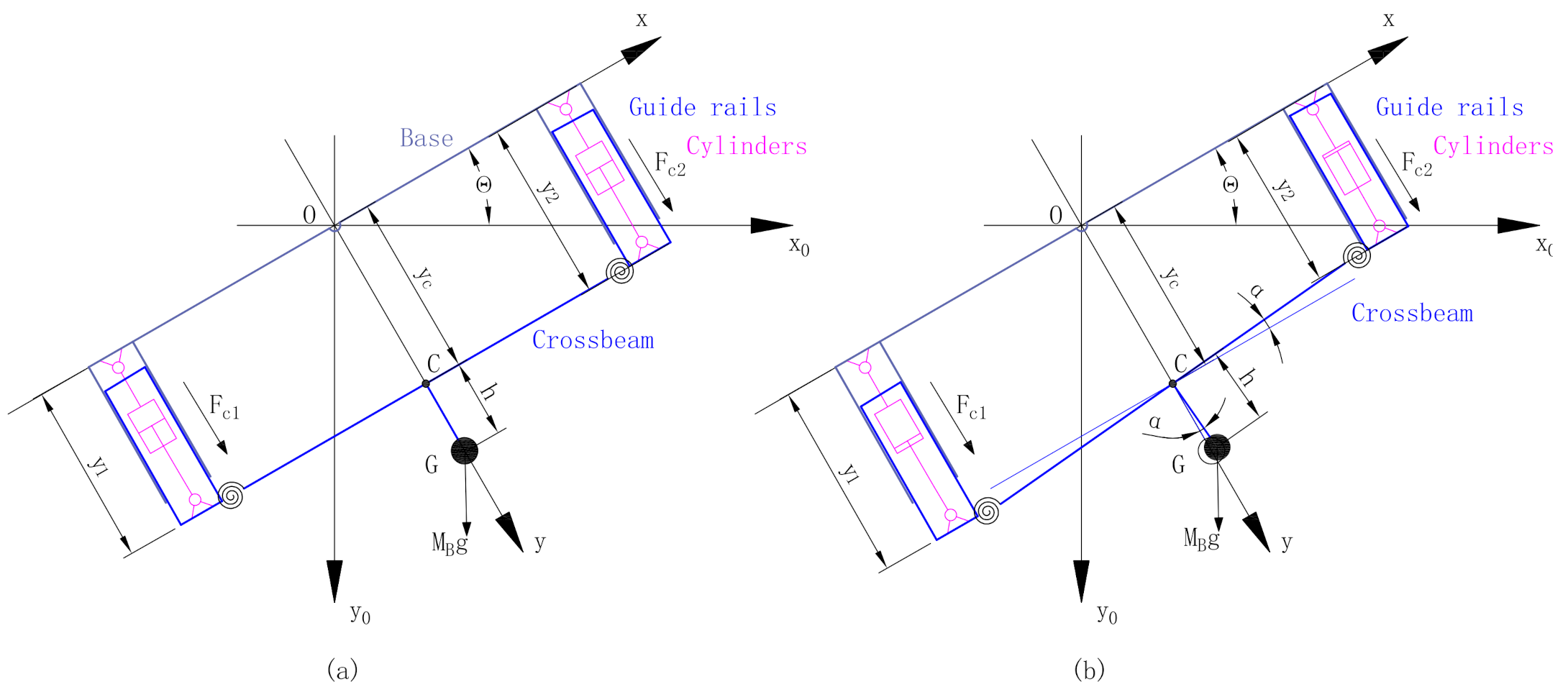
In order to analyze the complete behaviors of the lifting gantry, the schematic diagram is given in Figure 3. Figure 3a shows the general configuration of the lifting gantry, which follows the working principles of the actual gantry shown in Figure 2. $O{X}_0{Y}_0$ is the world coordinate frame, with its $Y_0$-axis vertically downwards and $X_0$-axis horizontal; $OXY$ is the coordinate frame attached to the lifting gantry, where its Y-axis is along the movement direction of the dual cylinders; and the angle $\Theta$ between the $X_0$-axis and X-axis shows that the whole lifting gantry usually works at an inclined angle. To illustrate the existing degree-of-freedom of crossbeam rotation, the relatively elastic part, which is the connection between the crossbeam and the guide rails, can be modeled as rotary springs with very large stiffness. With such a configuration, the complete planar motions of the entire moving body consist of the linear motion along the Y-axis, and an additional rotation of the crossbeam with a very small angle $\alpha$, which is illustrated in Figure 3b. Thus, the lifting gantry can be illustrated by a 2-DOF model. Other details and assumptions will be given in the next subsection.

The practical synchronization problem of the lifting gantry in the segment erector confirms the existence of crossbeam rotation. Thus, the proposed schematic diagram can be used to study the gantry since it includes the linear and rotational motions completely. However, achieving high-precision control of such a lifting gantry remains a challenging task, especially when it usually works at an inclined angle. Therefore, at the hardware level, the dual cylinders should be controlled by independent proportional valves in the hydraulic circuit, which will offer two independent control inputs to handle the 2-DOF model. On this basis, detailed modeling and model-based motion control design of the lifting gantry are the main contributions of this study.

2.2. Modeling of the Lifting Gantry

Figure 3b can be used to illustrate the modeling of the lifting gantry. The positions of the dual sides are defined as $y_1$ and $y_2$, separately; and the output cylinder rod forces are defined as $F_{c1}$ and $F_{c2}$, with the positive directions along the Y-axis. Point C denotes the midpoint of the crossbeam, and its position is written as $y_c$, which is also along the Y-axis. Point G is used to illustrate the centroid of the entire crossbeam, which should include the mass of the crossbeam itself and also the segment being lifted. Thus, point G should have a distance from point C, which is expressed as h. The angle $\alpha$ is used to describe the rotational motion of the crossbeam, which is defined as the angle between the actual crossbeam and the X-axis. In addition to the above definition, the following practical assumptions can be made.

Assumption 1.

The crossbeam with the attached segment is a perfectly rigid body. Thus, the line between the centroid G and the midpoint C is perpendicular to the crossbeam. Since the crossbeam and segment are very heavy, the mass of other parts such as the guide rails and the cylinders can be neglected.

Assumption 2.

The elasticity only comes from the connections between the crossbeam and the guide rails, even though the stiffness of the connection is very large, resulting in a very small rotational angle α, which is the truth in practice.

Assumption 3.

Due to the symmetrical structure of the lifting gantry, the midpoint C is always on the Y-axis.

Based on the aforementioned definitions and assumptions, the complete planar motions of the entire moving body in the frame $OXY$ consist of the linear motion along the Y-axis and an additional rotation around the midpoint C of the crossbeam. Thus, the generalized coordinates $q={[yc,\alpha ]}^T$ can be used to describe the 2-DOF motions. Since it is inconvenient to measure $y_c$ and $\alpha$ directly in practice, the following geometrical relationships can be used to calculate them by the measurement of $y_1$ and $y_2$

$$\begin{array}{cc}\hfill y_c& =\frac{1}{2}(y_1+y_2)\hfill \\ \hfill \alpha & \approx sin\alpha =\frac{1}{l_c}(y_1-y_2)\hfill \end{array}$$

(1)

with $l_c$ being the length of the crossbeam. Moreover, according to the geometrical relationships in Figure 3b, the coordinates of the centroid G ${[x_G,y_G]}^T$ can be written as

$$x_G=hsin\alpha ,y_G=y_c+hcos\alpha$$

(2)

then, the velocity of the centroid G can be calculated as

$$v_G={[{\dot{x}}_G,{\dot{y}}_G]}^T={[hcos\alpha \dot{\alpha },{\dot{y}}_c-hsin\alpha \dot{\alpha }]}^T$$

(3)

Thus, the kinetics energy including both the linear motion and the rotational motion can be expressed as

$$\begin{array}{cc}\hfill E_k& =\frac{1}{2}{m}_G{v}_G^T{v}_G+\frac{1}{2}{J}_G{\dot{\alpha }}^2\hfill \\ \hfill & =\frac{1}{2}{m}_G{\dot{y}}_c^2+\frac{1}{2}{m}_G{h}^2{\dot{\alpha }}^2+\frac{1}{2}{J}_G{\dot{\alpha }}^2-m_{G}hsin\alpha {\dot{y}}_c\dot{\alpha }\hfill \end{array}$$

(4)

with $m_G$ being the mass of the moving body including the crossbeam and the segment, and $J_G$ being the rotational inertia of the whole moving body around the centroid G. Moreover, the potential energy, including the gravitational energy $E_{pG}$ and elastic energy $E_{pE}$, can be calculated as

$$\begin{array}{cc}\hfill E_p& =E_{pG}+E_{pE}\hfill \\ \hfill & =-m_{G}g[y_{c}cos\Theta +hcos(\Theta +\alpha )]+\frac{1}{2}{k}_e{\alpha }^2\hfill \end{array}$$

(5)

where the gravitational energy takes the $X_0$-axis as the reference, and $k_e$ is the effective elastic stiffness of the connections between the crossbeam and guide rails. The model of the elastic energy $E_{pE}=\frac{1}{2}{k}_e{\alpha }^2$ is able to reflect the relationship between the internal forces and the rotational angle.

Defining $E=E_k-E_p$ as the Lagrangian function, using the Lagrangian Equation $\frac{d}{dt}\left(\frac{\partial E}{\partial {\dot{q}}_i}\right)-\frac{\partial E}{\partial q_i}=F_i,i=1,2$, the following equations can be generated:

$$\begin{array}{cc}\hfill m_G{\ddot{y}}_c-m_{G}gcos\Theta -m_{G}hsin\alpha ·\ddot{\alpha }-m_{G}hcos\alpha ·{\dot{\alpha }}^2& =F_1\hfill \\ \hfill (J_G+m_G{h}^2)\ddot{\alpha }+k_e\alpha -m_{G}hsin\alpha ·{\ddot{y}}_c-m_{G}hcos\alpha ·\dot{\alpha }·{\dot{y}}_c+m_{G}ghsin(\Theta +\alpha )& =F_2\hfill \end{array}$$

(6)

where $F_1$ and $F_2$ are the corresponding generalized forces and can be further written as

$$\begin{array}{cc}\hfill F_1& =F_{c1}+F_{c2}-F_{r1}-F_{r2}\hfill \\ \hfill F_2& =(F_{c1}-F_{c2}-F_{r1}+F_{r2})\frac{l_c}{2}\hfill \end{array}$$

(7)

with $F_{c1}$ and $F_{c2}$ being the output cylinder rod forces, which will be further discussed later, and $F_{r1}$ and $F_{r2}$ being the combined viscous and Coulomb friction forces of the two sides, which can be further expressed as

$$\begin{array}{cc}\hfill F_{r1}& =B_1{\dot{y}}_1+A_{1}S\left({\dot{y}}_1\right)\hfill \\ \hfill F_{r2}& =B_2{\dot{y}}_2+A_{2}S\left({\dot{y}}_2\right)\hfill \end{array}$$

(8)

in which $B_i$ and $A_i$ are the coefficients of viscous and Coulomb friction, and $S(•)$ is a continuous function used to approximate the sign function $sgn(•)$.

$F_{c1}$ and $F_{c2}$ are generated by hydraulic cylinders, and each cylinder is controlled by a proportional valve. Taking the cylinder C1 as an example, the output rod force can be modeled as

$$F_{c1}=p_{A1}{A}_{A1}-p_{B1}{A}_{B1}$$

(9)

with $A_{A1}$ and $A_{B1}$ being the piston areas of the head-end and rod-end chambers, respectively, and $p_{A1}$ and $p_{B1}$ being the pressure of each chamber, whose dynamics can be further expressed as

$$\begin{array}{cc}\hfill {\dot{p}}_{A1}& =-\frac{A_{A1}}{V_{A1}}{\beta }_e{\dot{y}}_1+\frac{1}{V_{A1}}{\beta }_e{Q}_{A1}+d_{A1}\hfill \\ \hfill {\dot{p}}_{B1}& =\frac{A_{B1}}{V_{B1}}{\beta }_e{\dot{y}}_1-\frac{1}{V_{B1}}{\beta }_e{Q}_{B1}+d_{B1}\hfill \end{array}$$

(10)

where $V_{A1}=V_{A10}+A_{A1}{y}_1$ and $V_{B1}=V_{B10}-A_{B1}{y}_1$ are the entire hydraulic compressible volumes corresponding to the head-end and rod-end chambers at the position $y_1$, $V_{A10}$ and $V_{B10}$ are the initial volumes, ${\beta }_e$ represents the effective bulk modulus, $Q_{A1}$ is the flow into the head-end chamber and $Q_{B1}$ is the flow out of the rod-end chamber, and $d_{A1}$ and $d_{B1}$ indicate the unavoidable modeling errors. Thus, the dynamics of $F_{c1}$ can be calculated as

$$\begin{array}{cc}\hfill {\dot{F}}_{c1}& ={\dot{p}}_{A1}{A}_{A1}-{\dot{p}}_{B1}{A}_{B1}\hfill \\ \hfill & =-(\frac{A_{A1}^2}{V_{A1}}+\frac{A_{B1}^2}{V_{B1}}){\beta }_e{\dot{y}}_1+{\beta }_e(\frac{A_{A1}}{V_{A1}}{Q}_{A1}+\frac{A_{B1}}{V_{B1}}{Q}_{B1})+A_{A1}{d}_{A1}-A_{B1}{d}_{B1}\hfill \end{array}$$

(11)

Considering the properties of the commonly used proportional directional valve, $Q_{A1}$ and $Q_{B1}$ can be further written as

$$\begin{array}{cc}\hfill Q_{A1}& =k_{qA1}{u}_1\sqrt{|\Delta p_{A1}|},\Delta p_{A1}=\left\{\begin{array}{cc}{p}_s-p_{A1},\hfill & u_1\ge 0\hfill \\ p_{A1},\hfill & u_1<0\hfill \end{array}\right.\hfill \\ \hfill Q_{B1}& =k_{qB1}{u}_1\sqrt{|\Delta p_{B1}|},\Delta p_{B1}=\left\{\begin{array}{cc}{p}_{B1},\hfill & u_1\ge 0\hfill \\ p_s-p_{B1},\hfill & u_1<0\hfill \end{array}\right.\hfill \end{array}$$

(12)

where $k_{qA1}$ and $k_{qB1}$ are the flow gains of the valve, $u_1$ is the control signal of the proportional valve, and $p_s$ and $p_r$ are the pressures of the pump and the tank. The dynamics between the control signal $u_1$ and the valve spool position are neglected because the bandwidth is high enough, as noted in many other existing works [30]. Noting (11) and (12), we can define an intermediate flow rate quantity $Q_{c1}$ as

$$Q_{c1}=\frac{A_{A1}}{V_{A1}}{Q}_{A1}+\frac{A_{B1}}{V_{B1}}{Q}_{B1}=(\frac{A_{A1}}{V_{A1}}{k}_{qA1}\sqrt{|\Delta p_{A1}|}+\frac{A_{B1}}{V_{B1}}{k}_{qB1}\sqrt{|\Delta p_{B1}|})u_1$$

(13)

which is a static projection of the control input $u_1$. Similarly, the other cylinder C2 can also be modeled as

$$\begin{array}{cc}\hfill {\dot{F}}_{c2}& ={\dot{p}}_{A2}{A}_{A2}-{\dot{p}}_{B2}{A}_{B2}\hfill \\ \hfill & =-(\frac{A_{A2}^2}{V_{A2}}+\frac{A_{B2}^2}{V_{B2}}){\beta }_e{\dot{y}}_2+{\beta }_e{Q}_{C2}+A_{A2}{d}_{A2}-A_{B2}{d}_{B2}\hfill \\ \hfill Q_{c2}& =(\frac{A_{A2}}{V_{A2}}{k}_{qA2}\sqrt{|\Delta p_{A2}|}+\frac{A_{B2}}{V_{B2}}{k}_{qB2}\sqrt{|\Delta p_{B2}|})u_2\hfill \end{array}$$

(14)

where $u_2$ is the control input of the proportional valve and other symbols have similar meanings to the ones in Equations (9)–(13).

To integrate the above modeling procedures, the dynamics of the lifting gantry can be reorganized as follows, considering the modeling errors:

$$\begin{array}{cc}\hfill m_G{\ddot{y}}_c& =F_{c1}+F_{c2}-F_{r1}-F_{r2}+m_{G}gcos\Theta +m_{G}h(sin\alpha ·\ddot{\alpha }+cos\alpha ·{\dot{\alpha }}^2)+d_{yc}\hfill \\ \hfill (J_G+m_G{h}^2)\ddot{\alpha }& =(F_{c1}-F_{c2}-F_{r1}+F_{r2})\frac{l_c}{2}-k_e\alpha +m_{G}h(sin\alpha ·{\ddot{y}}_c+cos\alpha ·\dot{\alpha }·{\dot{y}}_c)\hfill \\ \hfill & -m_{G}ghsin(\Theta +\alpha )+d_{\alpha }\hfill \\ \hfill {\dot{F}}_{c1}& =-(\frac{A_{A1}^2}{V_{A1}}+\frac{A_{B1}^2}{V_{B1}}){\beta }_e{\dot{y}}_1+{\beta }_e{Q}_{C1}+A_{A1}{d}_{A1}-A_{B1}{d}_{B1}\hfill \\ \hfill {\dot{F}}_{c2}& =-(\frac{A_{A2}^2}{V_{A2}}+\frac{A_{B2}^2}{V_{B2}}){\beta }_e{\dot{y}}_2+{\beta }_e{Q}_{C2}+A_{A2}{d}_{A2}-A_{B2}{d}_{B2}\hfill \end{array}$$

(15)

where $F_{r1}$ and $F_{r2}$ have been given in Equation (8), $d_{yc}$, $d_{\alpha }$, $d_{A1}$, $d_{B1}$, $d_{A2}$, and $d_{B2}$ represent the modeling errors of the corresponding dynamics equations, and $Q_{c1}$ and $Q_{c2}$ can be treated as the available control inputs since they are directly related to the real control inputs $u_1$ and $u_2$.

2.3. Synchronization Control Objectives

To achieve high-precision motion tracking performance of the dual-cylinder lifting gantry, while keeping the internal forces and rotational angle within a small range, a model-based motion synchronization control scheme is proposed in this study. The controller should synthesize the valve control signals $u_1$ and $u_2$ such that the following objectives can be fulfilled:

• High motion tracking precision: The midpoint position $y_c$ tracks the reference trajectory $y_d\left(t\right)$ as precisely as possible, which is assumed to be known, bounded, and at least third-order differentiable;
• Rotation regulation: The dual cylinders should be properly coordinated so that the rotational angle of the crossbeam can be guaranteed within a very small range.

3. Synchronization Control Schemes

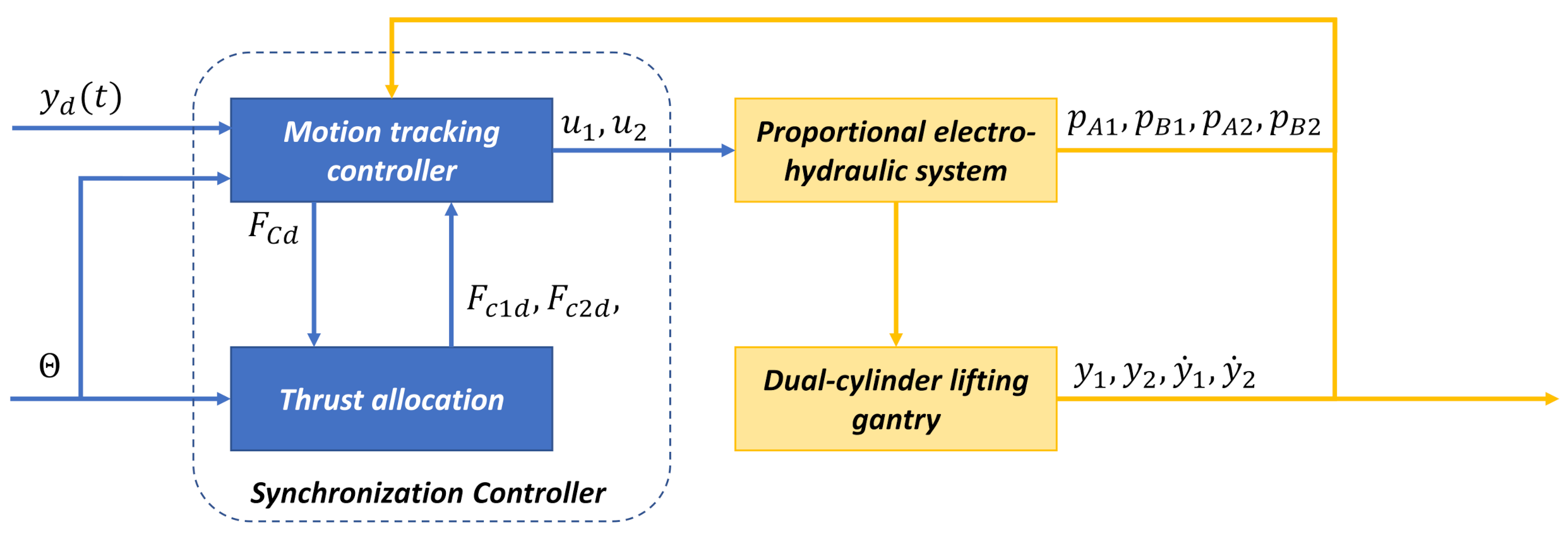
The structure of the proposed controller is shown in Figure 4. In terms of input signals, the controller receives the reference trajectory signals $y_d\left(t\right)$, the rotational angle $\Theta$ of the entire lifting gantry, and the state feedback signals from both the hydraulic system and the gantry. Based on such signals and the system model, the controller synthesizes the control signals $u_1$ and $u_2$. The controller contains two parts, i.e., a motion tracking controller and thrust allocation. The thrust allocation part is designed to coordinate the dual cylinders; it receives the angle $\Theta$ and the desired total force $F_{Cd}$ from the motion tracking controller and synthesizes the individual desired forces $F_{c1d}$ and $F_{c2d}$ for the dual cylinders. The motion tracking controller is the core of the entire controller, and it is developed based on the adaptive robust control theory proposed by Yao [20] to guarantee the desired tracking precision in the presence of parametric uncertainties and modeling errors. The details of the thrust allocation and motion tracking controller are provided in the following subsections.

3.1. Thrust Allocation

In order to avoid large internal forces and keep the rotational angle $\alpha$ within a small range, a practical thrust allocation scheme is developed in this study. Within the rotational dynamics in (22), i.e., the second equation in (22), $k_e\alpha$ can be treated as a proportional feedback term with a very large gain $k_e$. If we can keep $(F_{c1}-F_{c2}-F_{r1}+F_{r2})\frac{l_c}{2}-m_{G}ghsin(\Theta +\alpha )$ within a relatively small range, the angle $\alpha$ can also be regulated to be small in steady state, thanks to the existence of $k_e\alpha$. Therefore, both the rotational angle and the internal forces due to the mechanical coupling will be regulated to a level around zero.

Following the above idea, the practical thrust allocation scheme can be designed as follows. Define $F_{Cd}$, which will be detailed in the next subsection, as the desired force for $F_C$ to guarantee the tracking precision of the linear motion, i.e., $y_c$ tracks $y_d$ precisely. For the dual cylinders, the desired forces $F_{c1d}$ and $F_{c2d}$ of $F_{c1}$ and $F_{c2}$ should satisfy the following condition:

$$F_{c1d}+F_{c2d}=F_{Cd}$$

(16)

such that the linear motion tracking precision can be guaranteed. At the same time, in order to regulate the rotational angle, $F_{c1d}$ and $F_{c2d}$ should also satisfy

$$(F_{c1d}-F_{c2d}-F_{r1}+F_{r2})\frac{l_c}{2}-m_{G}ghsin(\Theta +\alpha )\approx 0$$

(17)

The pre-estimated friction forces can be used to precisely calculate $F_{c1d}$ and $F_{c2d}$. However, for simplicity, considering the fact that $F_{r1}$ and $F_{r2}$ are much smaller compared with $F_{c1d}$ and $F_{c2d}$ in practice, and noting Assumption 3, the following approximation can be used, because the large feedback gain $k_e$ is also able to regulate the angle $\alpha$ within a small range in the presence of some approximation errors:

$$(F_{c1d}-F_{c2d})\frac{l_c}{2}-m_{Gpre}ghsin(\Theta )\approx 0$$

(18)

with $m_{Gpre}$ being the pre-estimated mass of the entire moving body. Therefore, according to the relationships in (16) and (18), the desired forces for the dual cylinder can be allocated as

$$\begin{array}{cc}\hfill F_{c1d}& =\frac{1}{2}{F}_{Cd}+\frac{1}{l_c}{m}_{Gpre}ghsin(\Theta )\hfill \\ \hfill F_{c2d}& =\frac{1}{2}{F}_{Cd}-\frac{1}{l_c}{m}_{Gpre}ghsin(\Theta )\hfill \end{array}$$

(19)

The thrust allocation scheme above is practical for engineering applications. It is essentially an open-loop control of the rotational motion, and thus avoids the need for measurement signals of $\alpha$, which usually contains noise in practice. Based on the analysis, the thrust allocation scheme is able to regulate the rotational motion thanks to the inherent large stiffness of the connection itself. The relationship in (19) will be applied in the following subsection to finally synthesize the control signals $u_1$ and $u_2$.

3.2. Motion Tracking Controller

3.2.1. Parameterized System Dynamics for Control Design

Some simplifications have to be made in order to design the synchronization controller. In (15), the coupling term $m_{G}h(sin\alpha ·\ddot{\alpha }+cos\alpha ·{\dot{\alpha }}^2)$ is inconvenient to be compensated directly in control law because it consists of the second derivative of $\alpha$. In addition, the angle $\alpha$ is very small and may suffer from measurement noise in practice, so the achievable precision of the direct model compensation might not be satisfactory. Therefore, in this study, the influence of this coupling term will be lumped as an integrated term, which will be updated online and compensated as a whole through a well-designed adaptive control law.

On the basis of the model constructed in (15), the dynamics of linear motion along the Y-axis can be modified as

$${\ddot{y}}_c=gcos\Theta +\frac{1}{m_G}{F}_C-\frac{B_r}{m_G}{\dot{y}}_c-\frac{A_r}{m_G}S\left({\dot{y}}_c\right)+D_{1n}+\Delta D_1$$

(20)

where $F_C=F_{c1}+F_{c2}$, $B_r=B_1+B_2$, $A_r=A_1+A_2$, ${\dot{y}}_c$, instead of ${\dot{y}}_1$ and ${\dot{y}}_2$, is used to approximate the frictions for simplicity since $y_c\approx y_1\approx y_2$ under the small angle $\alpha$ assumption, and $D_1=D_{1n}+\Delta D_1$ represents the lumped disturbance term including the modeling errors, coupling terms, and the aforementioned friction approximation errors, with $D_{1n}$ being its nominal value. Then, following a similar procedure, the dynamics of the cylinder rod forces in (15) can be modified as

$$\begin{array}{cc}\hfill {\dot{F}}_{c1}& =-(\frac{A_{A1}^2}{V_{A1}}+\frac{A_{B1}^2}{V_{B1}}){\beta }_e{\dot{y}}_1+{\beta }_e{Q}_{C1}+A_{A1}{d}_{A1n}-A_{B1}{d}_{B1n}+\Delta d_{c1}\hfill \\ \hfill {\dot{F}}_{c2}& =-(\frac{A_{A2}^2}{V_{A2}}+\frac{A_{B2}^2}{V_{B2}}){\beta }_e{\dot{y}}_2+{\beta }_e{Q}_{C2}+A_{A2}{d}_{A2n}-A_{B2}{d}_{B2n}+\Delta d_{c2}\hfill \end{array}$$

(21)

where $d_{A1n}$, $d_{B1n}$, $d_{A2n}$, and $d_{B2n}$ are the nominal values of the modeling error terms in (15), and $\Delta d_{c1}$ and $\Delta d_{c2}$ represent the remaining lumped modeling errors.

As discussed in the last subsection, the thrust allocation will only use the static solution of the dynamics of the rotational motion; thus, the dynamics of the rotational motion do not need to be parameterized. According to (20) and (21), the parameterized model to be used in adaptive robust tracking control design can be derived as follows:

$$\begin{array}{cc}\hfill {\ddot{y}}_c& =gcos\Theta +{\theta }_1{F}_C-{\theta }_2{\dot{y}}_c-{\theta }_{3}S\left({\dot{y}}_c\right)+{\theta }_4+\Delta D_1\hfill \\ \hfill {\dot{F}}_{c1}& =-(\frac{A_{A1}^2}{V_{A1}}+\frac{A_{B1}^2}{V_{B1}}){\theta }_5{\dot{y}}_1+{\theta }_5{Q}_{C1}+A_{A1}{\theta }_6-A_{B1}{\theta }_7+\Delta d_{c1}\hfill \\ \hfill {\dot{F}}_{c2}& =-(\frac{A_{A2}^2}{V_{A2}}+\frac{A_{B2}^2}{V_{B2}}){\theta }_5{\dot{y}}_2+{\theta }_5{Q}_{C2}+A_{A2}{\theta }_8-A_{B2}{\theta }_9+\Delta d_{c2}\hfill \end{array}$$

(22)

where the parameters are defined as $\theta ={[{\theta }_1,{\theta }_2,...,{\theta }_9]}^T$, ${\theta }_1=1/m_G$, ${\theta }_2=B_r/m_G$, ${\theta }_3=A_r/m_G$, ${\theta }_4=D_{1n}$, ${\theta }_5={\beta }_e$, ${\theta }_6=d_{A1n}$, ${\theta }_7=d_{B1n}$, ${\theta }_8=d_{A2n}$, ${\theta }_9=d_{B2n}$. For the sake of simplicity, the following nomenclature is used throughout this paper: $\widehat{•}$ denotes the estimates of • with $\widetilde{•}$ being the estimation error, i.e., $\widetilde{•}=\widehat{•}-•$; ${•}_{min}$ and ${•}_{max}$ are the minimum and maximum values of $•\left(t\right)$ for all time t, respectively.

In (22), the unknown parameter $\theta$ and lumped modeling errors $\Delta D_1$, $\Delta d_{c1}$, and $\Delta d_{c2}$ all suffer from uncertainties in practice. However, the fact is that the parametric uncertainties and modeling errors are bounded with known bounds, which leads to the following practical assumption:

Assumption A4.

The extent of the parametric uncertainties and the modeling errors is known, i.e.,

$$\begin{array}{cc}\hfill & {\theta }_i\in {\Omega }_{{\theta }_i}\stackrel{\Delta }{=}\left\{{\theta }_i:{\theta }_{imin}\le {\theta }_i\le {\theta }_{imax}\right\}\hfill \\ \hfill & \Delta D_i\in {\Omega }_{D_i}\stackrel{\Delta }{=}\left\{\Delta D_i:\left|\Delta D_i\right|\le {\delta }_i\right\}\hfill \\ \hfill & \Delta d_{ci}\in {\Omega }_{d_{ci}}\stackrel{\Delta }{=}\left\{\Delta d_{ci}:\left|\Delta d_{ci}\right|\le {\delta }_{ci}\right\}\hfill \end{array}$$

(23)

where ${\theta }_{imin}={\left[{\theta }_{1min},{\theta }_{2min},···,{\theta }_{9min}\right]}^T$, ${\theta }_{imax}=[{\theta }_{1max},$${\theta }_{2max},···,{\theta }_{9max}{]}^T$ are the known bounds, and ${\delta }_i$ and ${\delta }_{ci}$ are known functions.

3.2.2. Adaptive Robust Motion Tracking Control Design

The Adaptive Robust Control (ARC) proposed by Yao [20] is used to synthesize the motion tracking controller. The parameters will be updated online by the use of the following discontinuous projection-type adaption law:

$$\dot{\widehat{\theta }}=Pro{j}_{\widehat{\theta }}\left(\Gamma \tau \right)$$

(24)

with $\Gamma$ being a positively defined diagonal adaption rate matrix, $\tau$ being an adaption function to be synthesized during the control design procedure, and the projection mapping function being

$$Pro{j}_{{\widehat{\theta }}_i}\left({•}_i\right)=\left\{\begin{array}{c}\begin{array}{cc}0,& if{\widehat{\theta }}_i={\theta }_{imax}and{•}_i>0\end{array}\\ \begin{array}{cc}0,& if{\widehat{\theta }}_i={\theta }_{imin}and{•}_i<0\end{array}\\ \begin{array}{cc}{•}_i,& \begin{array}{cccc}otherwise& & & \end{array}\end{array}\end{array}\right.$$

(25)

Therefore, the following properties can be guaranteed for any adaption function $\tau$ when (25) is used:

$$\begin{array}{cc}\hfill & \left(P1\right):\widehat{\theta }\in {\Omega }_{\theta }\stackrel{\Delta }{=}\left\{{\widehat{\theta }}_i:{\theta }_{imin}\le \widehat{\theta }\le {\theta }_{imax}\right\}\hfill \\ \hfill & \left(P2\right):{\tilde{\theta }}^T({\Gamma }^{-1}Pro{j}_{\widehat{\theta }}(\Gamma \tau )-\tau )\le 0,\forall \tau \hfill \end{array}$$

(26)

Then, a backstepping design for the adaptive robust motion tracking controller will be synthesized. The objective of the controller is to synthesize the valve control signals $u_1$ and $u_2$ such that the midpoint of the crossbeam $y_c$ tracks the given reference trajectory $y_d\left(t\right)$ as precisely as possible.

Step 1

Define the motion tracking error as $z_1=y_c-y_d$. Then, the following switching-function-like quantity can be defined

$$z_2={\dot{z}}_1+k_1{z}_1={\dot{x}}_L-{\dot{x}}_{eq},{\dot{x}}_{eq}\triangleq {\dot{x}}_d-k_1{z}_1$$

(27)

where $k_1>0$. Apparently, making $z_1$ small or converging to zero is equivalent to making $z_2$ small or converging to zero [20].

Noting (22), the dynamics of $z_2$ can be calculated as

$${\dot{z}}_2=gcos\Theta +{\theta }_1{F}_C-{\theta }_2{\dot{y}}_c-{\theta }_{3}S\left({\dot{y}}_c\right)+{\theta }_4+\Delta D_1-{\ddot{y}}_{eq}$$

(28)

where $F_C$ can be taken as the virtual control input to make $z_2$ small or converging to zero. Thus, following the ARC design procedure, the virtual control law $F_{Cd}$ for $F_C$ can be synthesized as

$$\begin{array}{cc}\hfill F_{Cd}& =F_{Cda}+F_{Cds}\hfill \\ \hfill F_{Cda}& =\frac{1}{{\widehat{\theta }}_1}[-gcos\Theta +{\widehat{\theta }}_2{\dot{y}}_c+{\widehat{\theta }}_{3}S\left({\dot{y}}_c\right)-{\widehat{\theta }}_4+{\ddot{y}}_{eq}]\hfill \\ \hfill F_{Cds}& =F_{Cds1}+F_{Cds2}\hfill \\ \hfill F_{Cds}& =-k_{2s1}\frac{1}{{\theta }_{1min}}{z}_2,,k_{2s1}\ge \frac{{\omega }_3}{{\omega }_2}{g}_1{\Vert \Gamma {\varphi }_1{\omega }_2\Vert }^2+k_2\hfill \\ \hfill {\varphi }_1& ={[F_{Cda},-{\dot{y}}_c,-S\left({\dot{y}}_c\right),1,0,0,0,0,0]}^T\hfill \end{array}$$

(29)

where the control law $F_{Cd}$ includes the adaptive model compensation law $F_{Cda}$ and the robust control law $F_{Cds}$, in which $k_{2s1}>0$ is the feedback gain, $k_2>0$ and $g_1>0$, $\Gamma >0$ is the adaption rate matrix, ${\omega }_2>0$ and ${\omega }_3>0$ are the weighting coefficients, and $F_{Cds2}$ is the nonlinear robust feedback term satisfying the following dual robust performance conditions:

$$\begin{array}{cc}\hfill & \left(i\right)z_2{F}_{Cds2}\le 0\hfill \\ \hfill & \left(ii\right)z_2({\theta }_1{F}_{Cds2}-{\varphi }_1^T\tilde{\theta }+\Delta D_1)\le {\epsilon }_1\hfill \end{array}$$

(30)

with ${\epsilon }_1$ being a design parameter.

Define the discrepancy between the actual cylinder force $F_C$ and the virtual control law $F_{Cd}$ as $z_3=F_C-F_{Cd}$. Then, substituting (29) into (28), the resulting error dynamics of $z_2$ can be calculated as

$${\dot{z}}_2=-\frac{{\theta }_1}{{\theta }_{1min}}{k}_{2s1}{z}_2+({\theta }_1{F}_{Cds2}-{\varphi }_1^T\tilde{\theta }+\Delta D_1)+{\theta }_1{z}_3$$

(31)

Step 2

This step is to synthesize the control signals $u_1$ and $u_2$ for the proportional valves. Define the following tracking errors as

$$\begin{array}{cc}\hfill z_3& \triangleq z_{31}+z_{32}\hfill \\ \hfill z_{31}& =F_{c1}-F_{c1d}\hfill \\ \hfill z_{32}& =F_{c2}-F_{c2d}\hfill \end{array}$$

(32)

where $F_{c1d}$ and $F_{c2d}$ are given in (19). Noting (22) and (29), the derivative of $z_{31}$ can be calculated as

$$\begin{array}{cc}\hfill {\dot{z}}_{31}& ={\dot{F}}_{c1}-{\dot{F}}_{c1d}\hfill \\ \hfill & =-(\frac{A_{A1}^2}{V_{A1}}+\frac{A_{B1}^2}{V_{B1}}){\theta }_5{\dot{y}}_1+{\theta }_5{Q}_{C1}+A_{A1}{\theta }_6-A_{B1}{\theta }_7+\Delta d_{c1}-\frac{1}{2}{\dot{F}}_{Cd}\hfill \end{array}$$

(33)

with ${\dot{F}}_{Cd}$ being the derivative of $F_{Cd}$ defined in (29). Then, ${\dot{F}}_{Cd}$ can be written as the sum of two parts as

$$\begin{array}{cc}\hfill {\dot{F}}_{Cd}& ={\dot{F}}_{Cdc}+{\dot{F}}_{Cdu}\hfill \\ \hfill {\dot{F}}_{Cdc}& =\frac{\partial F_{Cd}}{\partial y_c}{\dot{y}}_c+\frac{\partial F_{Cd}}{\partial {\dot{y}}_c}{\widehat{\ddot{y}}}_c+\frac{\partial F_{Cd}}{\partial t}\hfill \\ \hfill {\widehat{\ddot{y}}}_c& =gcos\Theta +{\widehat{\theta }}_1{F}_C-{\widehat{\theta }}_2{\dot{y}}_c-{\widehat{\theta }}_{3}S\left({\dot{y}}_c\right)+{\widehat{\theta }}_4\hfill \\ \hfill {\dot{F}}_{Cdi}& =\frac{\partial F_{Cd}}{\partial {\dot{y}}_c}({\ddot{y}}_c-{\widehat{\ddot{y}}}_c)+\frac{\partial F_{Cd}}{\partial \widehat{\theta }}\dot{\widehat{\theta }}\hfill \\ \hfill & =\frac{\partial F_{Cd}}{\partial {\dot{y}}_c}[-{\tilde{\theta }}_1{F}_C+{\tilde{\theta }}_2{\dot{y}}_c+{\tilde{\theta }}_{3}S\left({\dot{y}}_c\right)-{\tilde{\theta }}_4+\Delta D_1]+\frac{\partial F_{Cd}}{\partial \widehat{\theta }}\dot{\widehat{\theta }}\hfill \end{array}$$

(34)

where ${\dot{F}}_{Cdc}$ represents the calculable part of ${\dot{F}}_{Cd}$, which can be compensated through adaptive robust control law, ${\widehat{\ddot{y}}}_c$ denotes the estimate of ${\ddot{y}}_c$ according to the measured states and parameter estimates, and ${\dot{F}}_{Cdi}$ is the incalculable part and has to be handled through a certain robust feedback approach.

Following the ARC design procedure, noting the error dynamics in (33), the control law $Q_{c1d}$ for $Q_{c1}$ can be synthesized as

$$\begin{array}{cc}\hfill Q_{c1d}& =Q_{c1da}+Q_{c1ds}\hfill \\ \hfill Q_{c1da}& =\frac{1}{{\widehat{\theta }}_5}[(\frac{A_{A1}^2}{V_{A1}}+\frac{A_{B1}^2}{V_{B1}}){\widehat{\theta }}_5{\dot{y}}_1-A_{A1}{\widehat{\theta }}_6-A_{B1}{\widehat{\theta }}_7+\frac{1}{2}{\dot{F}}_{Cdc}-\frac{{\omega }_2}{2{\omega }_3}{\widehat{\theta }}_1{z}_2]\hfill \\ \hfill Q_{c1ds}& =Q_{c1ds1}+Q_{c1ds2}\hfill \\ \hfill Q_{c1ds1}& =-k_{3s1}\frac{1}{{\theta }_{5min}}{z}_{31},k_{3s1}\ge g_2\Vert \Gamma {\varphi }_2{\omega }_3{\Vert }^2+c_1{\Vert \frac{\partial F_{Cd}}{\partial \widehat{\theta }}\Vert }^2+k_3\hfill \end{array}$$

(35)

where the control law $Q_{c1d}$ includes the adaptive model compensation law $Q_{c1da}$ and the robust control law $Q_{c1ds}$, in which $k_{3s1}>0$ is the feedback gain, $k_3>0$, $g_2>0$, $d_1>0$, $\Gamma >0$ is the adaption rate matrix, and $Q_{c1ds2}$ is the nonlinear robust feedback term to be detailed later.

Similarly, the control law $Q_{c2d}$ for $Q_{c2}$ can also be synthesized with regard to the error $z_{32}$ as follows and the detailed procedure is omitted here:

$$\begin{array}{cc}\hfill Q_{c2d}& =Q_{c2da}+Q_{c2ds}\hfill \\ \hfill Q_{c2da}& =\frac{1}{{\widehat{\theta }}_5}[(\frac{A_{A2}^2}{V_{A2}}+\frac{A_{B2}^2}{V_{B2}}){\widehat{\theta }}_5{\dot{y}}_2-A_{A2}{\widehat{\theta }}_8-A_{B2}{\widehat{\theta }}_9+\frac{1}{2}{\dot{F}}_{Cdc}-\frac{{\omega }_2}{2{\omega }_3}{\widehat{\theta }}_1{z}_2]\hfill \\ \hfill Q_{c2ds}& =Q_{c2ds1}+Q_{c2ds2}\hfill \\ \hfill Q_{c2ds1}& =-k_{3s1}\frac{1}{{\theta }_{5min}}{z}_{32},k_{3s1}\ge g_2\Vert \Gamma {\varphi }_2{\omega }_3{\Vert }^2+c_1{\Vert \frac{\partial F_{Cd}}{\partial \widehat{\theta }}\Vert }^2+k_3\hfill \end{array}$$

(36)

with similar definitions to (35).

Noting $z_3=z_{31}+z_{32}$ and (22), the resulting error dynamics of $z_3$ can be calculated as follows using the control law in (35) and (36):

$$\begin{array}{cc}\hfill {\dot{z}}_3& =({\dot{F}}_{c1}-{\dot{F}}_{c1d})+({\dot{F}}_{c2}-{\dot{F}}_{c2d})\hfill \\ \hfill & =-k_{3s1}\frac{{\theta }_5}{{\theta }_{5min}}{z}_3+[{\theta }_5(Q_{c1ds2}+Q_{c2ds2})-{\varphi }_2^T\tilde{\theta }+\Delta d_{c1}+\Delta d_{c2}]-\frac{\partial F_{Cd}}{\partial \widehat{\theta }}\dot{\widehat{\theta }}-\frac{{\omega }_2}{{\omega }_3}{\theta }_1{z}_2\hfill \end{array}$$

(37)

where the regressor ${\varphi }_2$ is written as

$${\varphi }_2=\left[\begin{array}{c}\frac{{\omega }_2}{{\omega }_3}{z}_2-\frac{\partial F_{Cd}}{\partial {\dot{y}}_c}{F}_C\\ \frac{\partial F_{Cd}}{\partial {\dot{y}}_c}{\dot{y}}_c\\ \frac{\partial F_{Cd}}{\partial {\dot{y}}_c}S\left({\dot{y}}_c\right)\\ -\frac{\partial F_{Cd}}{\partial {\dot{y}}_c}\\ -(\frac{A_{A1}^2}{V_{A1}}+\frac{A_{B1}^2}{V_{B1}}){\dot{y}}_1-(\frac{A_{A2}^2}{V_{A2}}-\frac{A_{B2}^2}{V_{B2}}){\dot{y}}_2+Q_{c1da}+Q_{c2da}\\ A_{A1}\\ A_{B1}\\ A_{A2}\\ A_{B2}\end{array}\right]$$

(38)

The nonlinear robust feedback terms $Q_{c1ds2}$ and $Q_{c2ds2}$ are chosen so that the following dual robust conditions are satisfied:

$$\begin{array}{cc}\hfill & \left(i\right)z_3(Q_{c1ds2}+Q_{c2ds2})\le 0\hfill \\ \hfill & \left(ii\right)z_3[{\theta }_5(Q_{c1ds2}+Q_{c2ds2})-{\varphi }_2^T\tilde{\theta }+\Delta d_{c1}+\Delta d_{c2}]\le {\epsilon }_2\hfill \end{array}$$

(39)

where ${\epsilon }_2$ is a design parameter.

In addition, the unknown parameter set $\theta$ is estimated online using the discontinuous projection-type adaption law in (24), where the adaption function is defined as

$$\tau ={\omega }_2{\varphi }_1{z}_2+{\omega }_3{\varphi }_2{z}_3$$

(40)

Noting the relationship defined in (13) and (14) and the control law synthesized in (35) and (36), the valve control signals $u_1$ and $u_2$ can be generated finally as

$$\begin{array}{cc}\hfill u_1& =\frac{Q_{c1d}}{\frac{A_{A1}}{V_{A1}}{k}_{qA1}\sqrt{|\Delta p_{A1}|}+\frac{A_{B1}}{V_{B1}}{k}_{qB1}\sqrt{|\Delta p_{B1}|}}\hfill \\ \hfill u_2& =\frac{Q_{c2d}}{\frac{A_{A2}}{V_{A2}}{k}_{qA2}\sqrt{|\Delta p_{A2}|}+\frac{A_{B2}}{V_{B2}}{k}_{qB2}\sqrt{|\Delta p_{B2}|}}\hfill \\ \hfill \end{array}$$

(41)

3.2.3. Theoretical Performance

The following theoretical performance can be guaranteed with the resulting control law in (41).

Theorem 1.

If the controller parameters $g_1$, $g_2$, and $c_1$ satisfy $g_1>\frac{2}{4c_1}$ and $g_2>\frac{2}{4c_1}$, the control law in (41) with the adaption law in (24) leads to guaranteed tracking errors bounded by

$$V\left(t\right)\le exp(-\lambda t)V\left(0\right)+\frac{\epsilon }{\lambda }[1-exp(-\lambda t)]$$

(42)

where $V=\frac{1}{2}{\omega }_2{z}_2^2+\frac{1}{2}{\omega }_3{z}_3^2$, $\lambda =2\times min\{k_2,k_3\}$, $\epsilon ={\omega }_2{\epsilon }_1+{\omega }_3{\epsilon }_2$. In addition, if after a finite time $t_0$, $\Delta D_1=\Delta d_{c1}=\Delta d_{c2}=0$, i.e., in the presence of parametric uncertainties only, asymptotic output tracking is achieved, i.e., $z_1\to 0$ as $t\to \infty$.

Proof of Theorem 1. 

Differentiating $V\left(t\right)$ while noting the resulting error dynamics in (31) and (37), one can obtain

$$\begin{array}{cc}\hfill \dot{V}& ={\omega }_2{z}_2{\dot{z}}_2+{\omega }_3{z}_3{\dot{z}}_3\hfill \\ \hfill & =-{\omega }_2\frac{{\theta }_1}{{\theta }_{1min}}{k}_{2s1}{z}_2^2+{\omega }_2{z}_2({\theta }_1{F}_{Cds2}-{\varphi }_1^T\tilde{\theta }+\Delta D_1)-{\omega }_3\frac{{\theta }_5}{{\theta }_{5min}}{k}_{3s1}{z}_3^2\hfill \\ \hfill & +{\omega }_3{z}_3[{\theta }_5(Q_{c1ds2}+Q_{c2ds2})-{\varphi }_2^T\tilde{\theta }+\Delta d_{c1}+\Delta d_{c2}]-{\omega }_3{z}_3\frac{\partial F_{Cd}}{\partial \widehat{\theta }}\dot{\widehat{\theta }}\hfill \end{array}$$

(43)

In terms of the adaption law in (24), the following property is held:

$$\begin{array}{cc}\hfill \parallel \dot{\widehat{\theta }}{\parallel }^2& =\parallel Pro{j}_{\theta }[\Gamma ({\omega }_2{\varphi }_1{z}_2+{\omega }_3{\varphi }_2{z}_3)]{\parallel }^2\hfill \\ \hfill & \le \parallel \Gamma ({\omega }_2{\varphi }_1{z}_2+{\omega }_3{\varphi }_2{z}_3){\parallel }^2\hfill \\ \hfill & \le 2(\parallel \Gamma {\varphi }_1{\parallel }^2{\omega }_2^2{z}_2^2+\parallel \Gamma {\varphi }_2{\parallel }^2{\omega }_3^2{z}_3^2)\hfill \end{array}$$

(44)

Noting $g_1>\frac{2}{4c_1}$ and $g_2>\frac{2}{4c_1}$ and (44), the following relationship can be obtained:

$$\begin{array}{cc}\hfill |z_3\frac{\partial F_{Cd}}{\partial \widehat{\theta }}\dot{\widehat{\theta }}|& \le c_1\parallel \frac{\partial F_{Cd}}{\partial \widehat{\theta }}{\parallel }^2+\frac{1}{4c_1}{\parallel \dot{\widehat{\theta }}\parallel }^2\hfill \\ \hfill & \le d_1\parallel \frac{\partial F_{Cd}}{\partial \widehat{\theta }}{\parallel }^2+g_1\parallel \Gamma {\varphi }_1{\parallel }^2{\omega }_2^2{z}_2^2+g_2{\parallel \Gamma {\varphi }_2\parallel }^2{\omega }_3^2{z}_3^2\hfill \end{array}$$

(45)

Thus, substituting (45) into (43) and noting the inequalities in (29), (35), and (36) as well as the robust performance conditions in (30) and (39), the derivative of $V\left(t\right)$ becomes

$$\begin{array}{cc}\hfill \dot{V}& \le -{\omega }_2\frac{{\theta }_1}{{\theta }_{1min}}{k}_2{z}_2^2+{\omega }_2{z}_2({\theta }_1{F}_{Cds2}-{\varphi }_1^T\tilde{\theta }+\Delta D_1)-{\omega }_3\frac{{\theta }_5}{{\theta }_{5min}}{k}_3{z}_3^2\hfill \\ \hfill & +{\omega }_3{z}_3[{\theta }_5(Q_{c1ds2}+Q_{c2ds2})-{\varphi }_2^T\tilde{\theta }+\Delta d_{c1}+\Delta d_{c2}]\hfill \\ \hfill & \le -{\omega }_2{k}_2{z}_2^2-{\omega }_3{k}_3{z}_3^2+{\omega }_2{\epsilon }_1+{\omega }_3{\epsilon }_2\hfill \\ \hfill & =-\lambda V+\epsilon \hfill \end{array}$$

(46)

which leads to (42) by Comparison Lemma.

If $\Delta D_1=\Delta d_{c1}=\Delta d_{c2}=0$, one can define another positive-definite Lyapunov function as $V_{\theta }=V+\frac{1}{2}{\tilde{\theta }}^T{\Gamma }^{-1}\tilde{\theta }$. Noting the properties in (26), the relationship in (45), and ${\dot{\tilde{\theta }}}_{m1}={\dot{\widehat{\theta }}}_{m1}$, the derivative of $V_{\theta }$ is given as

$$\begin{array}{cc}\hfill {\dot{V}}_{\theta }& =\dot{V}+{\tilde{\theta }}^T{\Gamma }^{-1}\dot{\tilde{\theta }}\hfill \\ \hfill & =-{\omega }_2\frac{{\theta }_1}{{\theta }_{1min}}{k}_{2s1}{z}_2^2+{\omega }_2{z}_2{\theta }_1{F}_{Cds2}-{\omega }_3\frac{{\theta }_5}{{\theta }_{5min}}{k}_{3s1}{z}_3^2+{\omega }_3{z}_3{\theta }_5(Q_{c1ds2}+Q_{c2ds2})\hfill \\ \hfill & -\frac{\partial F_{Cd}}{\partial \widehat{\theta }}\dot{\widehat{\theta }}+{\tilde{\theta }}^T{\Gamma }^{-1}[\dot{\tilde{\theta }}-\Gamma ({\omega }_2{\varphi }_1{z}_2+{\omega }_3{\varphi }_2{z}_3)]\hfill \\ \hfill & \le -{\omega }_2{k}_2{z}_2^2-{\omega }_3{k}_3{z}_3^2+{\tilde{\theta }}^T[{\Gamma }^{-1}Pro{j}_{\theta }(\Gamma \tau )-\tau ]\hfill \\ \hfill & \le -{\omega }_2{k}_2{z}_2^2-{\omega }_3{k}_3{z}_3^2\hfill \end{array}$$

(47)

Thus, $z_2,z_3\in L_2$ and ${\dot{z}}_2$ and ${\dot{z}}_3$ are bounded. By Barbalat Lemma, $z_2\to 0$ as $t\to \infty$. Considering the stable transfer function between $z_1$ and $z_2$ in (27), one can obtain $z_1\to 0$ as $t\to \infty$. □

4. Simulation

4.1. Simulation Setups

The complete dynamics model built in (15) was used in Matlab/Simulink to establish the dynamics of the lifting gantry to be controlled, i.e., the plant. As for the principal parameters of the gantry, $m_G=2200\mathrm{kg}$, $B_1=1200\mathrm{N}/(\mathrm{m}/\mathrm{s})$, $B_2=800\mathrm{N}/(\mathrm{m}/\mathrm{s})$, $A_1=2000\mathrm{N}$, $A_2=1400\mathrm{N}$, $l_m=3\mathrm{m}$, $J_G=4000\mathrm{kg}·{\mathrm{m}}^2$, $k_e=1\times {10}^7\mathrm{Nm}/\mathrm{rad}$, $h=0.2\mathrm{m}$; and as for the cylinders, the diameters of the pistons were $80\mathrm{mm}$ and the diameters of the rods were $56\mathrm{mm}$. In addition, modeling errors were also added into all equations and the parameters used in the controller deviate from these true values in the plant.

The theoretically rigorous way to choose the controller parameters is demonstrated in [20], but it may increase the complexity of the resulting control law considerably. Thus, following our previous works [32,33], an alternative approach was used for gain tuning in this study by simply choosing $k_{2s1}$ and $k_{3s1}$ large enough without worrying about the precise values of the nonlinear robust feedbacks in (30) and (39). Such an approach was also used in [20,34]. By doing so, the robust performance conditions (30) and (39) were still satisfied at least locally around the reference trajectory.

The following three control schemes were compared in the simulation:

• C1: the proposed controller As for the thrust allocation, the pre-estimated mass of the entire moving body was chosen as $m_{Gpre}=2000\mathrm{kg}$, which deviated from the true value in the plant. In the motion tracking controller, the feedback gains were tuned as $k_1=k_{2s1}=k_{3s1}=50$; the adaption rate matrix was $\Gamma =diag\{5\times {10}^{-17},1\times {10}^{-9},1\times {10}^{-9},5\times {10}^{-9},4\times {10}^7,1\times {10}^7,1\times {10}^7,1\times {10}^7,1\times {10}^7\}$; and the weighting coefficients were ${\omega }_2=1\times {10}^{10}$ and ${\omega }_3=1$.
• C2: the controller without adaption The only difference from C1 was that the adaption in the motion tracking controller was turned off, i.e., $\Gamma$ was set to zero.
• C3: the controller without thrust allocation The dual cylinders were controlled by the same signals, which is the usual case in engineering. Thus, no efforts were made in the controller for synchronization. The dual cylinders had to be synchronized by the high-stiffness mechanical coupling itself. The motion tracking controller was exactly the same as the one in C1.

The above control schemes to be compared were chosen for the following reasons. As for C2, the adaptation is turned off, which causes it to behave similarly to a typical robust controller with only offline model compensation. Thus, by comparing C1 and C2, the effect of parameter adaptation can be inspected, e.g., in terms of steady-state tracking error or positioning error. As for C3, it can be treated as a commonly used control scheme in practical engineering. On one hand, in almost all engineering applications at present, the dual cylinders in the lifting gantry are controlled by a single human-operated proportional valve. This means that the synchronization is only ensured by the guide rails and crossbeam mechanically, while no efforts are made in the software or at the control level. Under such conditions, the forces of the dual cylinders should be the same, which will cause the crossbeam to rotate by a small angle and lead to synchronization problems. Thus, in C3, $F_{c1d}=F_{c2d}=\frac{1}{2}{F}_{Cd}$ instead of the proposed thrust allocation in (19) is used to generate the desired cylinder forces, which will lead to similar cylinder output forces to simulate the aforementioned practical situation. On the other hand, in practice, the PID control is usually used, and, intuitively, it seems that PID control should also be used in C3. However, the better performance of ARC over PID has been verified by many existing works [20]; ensuring the optimal parameter tuning of PID is time-consuming and also depends on the real task. If C3 uses PID, it will possibly be difficult to identify whether the improvement comes from ARC over PID or the proposed thrust allocation scheme. Therefore, C3 applies the proposed motion tracking controller but without thrust allocation to test the synchronization performance. Based on the above analyses, C2 and C3 are representative control schemes to compare with the proposed control scheme in terms of specific aspects.

As shown in Figure 5, a smoothed point-to-point S-curve reference trajectory was used in the simulation. The distance was set as 0.8 m, with a maximum velocity of 0.2 m/s and a maximum acceleration of 0.2 m/s ${}^2$. In addition, the simulations were conducted with different inclined angles $\Theta$ of the entire lifting gantry to test the synchronization performance under unbalanced loads. Specifically, there were three simulation sets, and $\Theta$ = 0, 0.5 rad, 1 rad were used in Set 1, Set 2, and Set 3, respectively.

4.2. Simulation Results

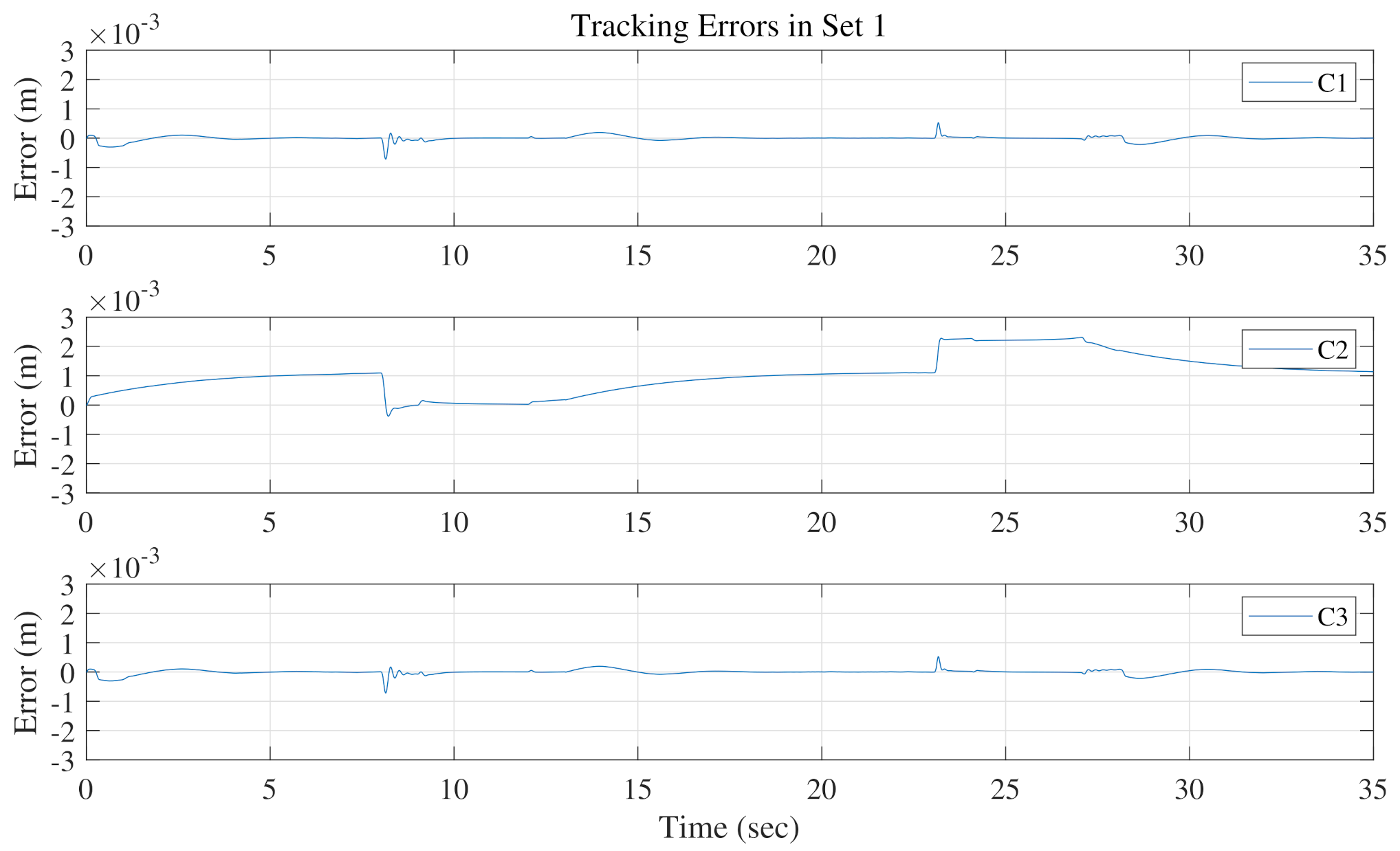
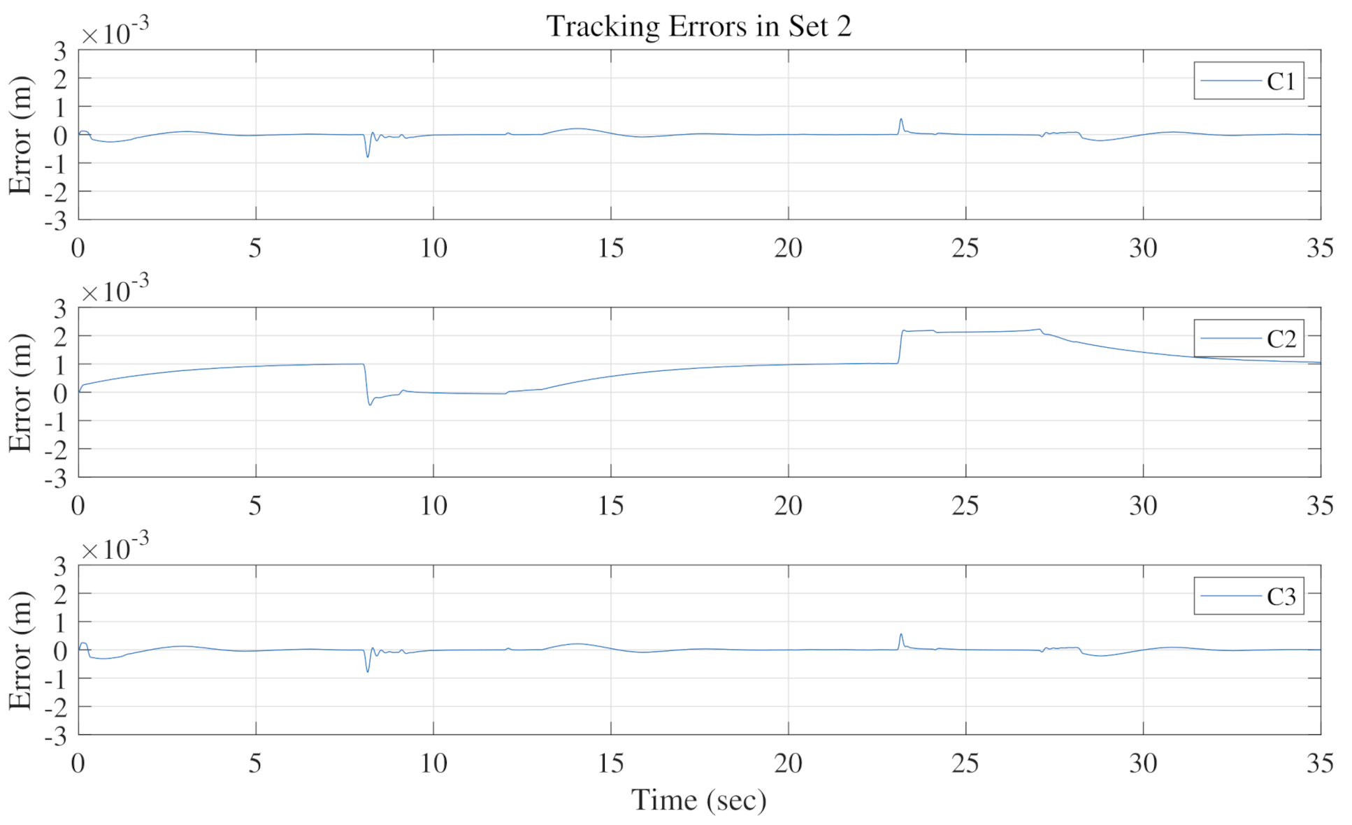
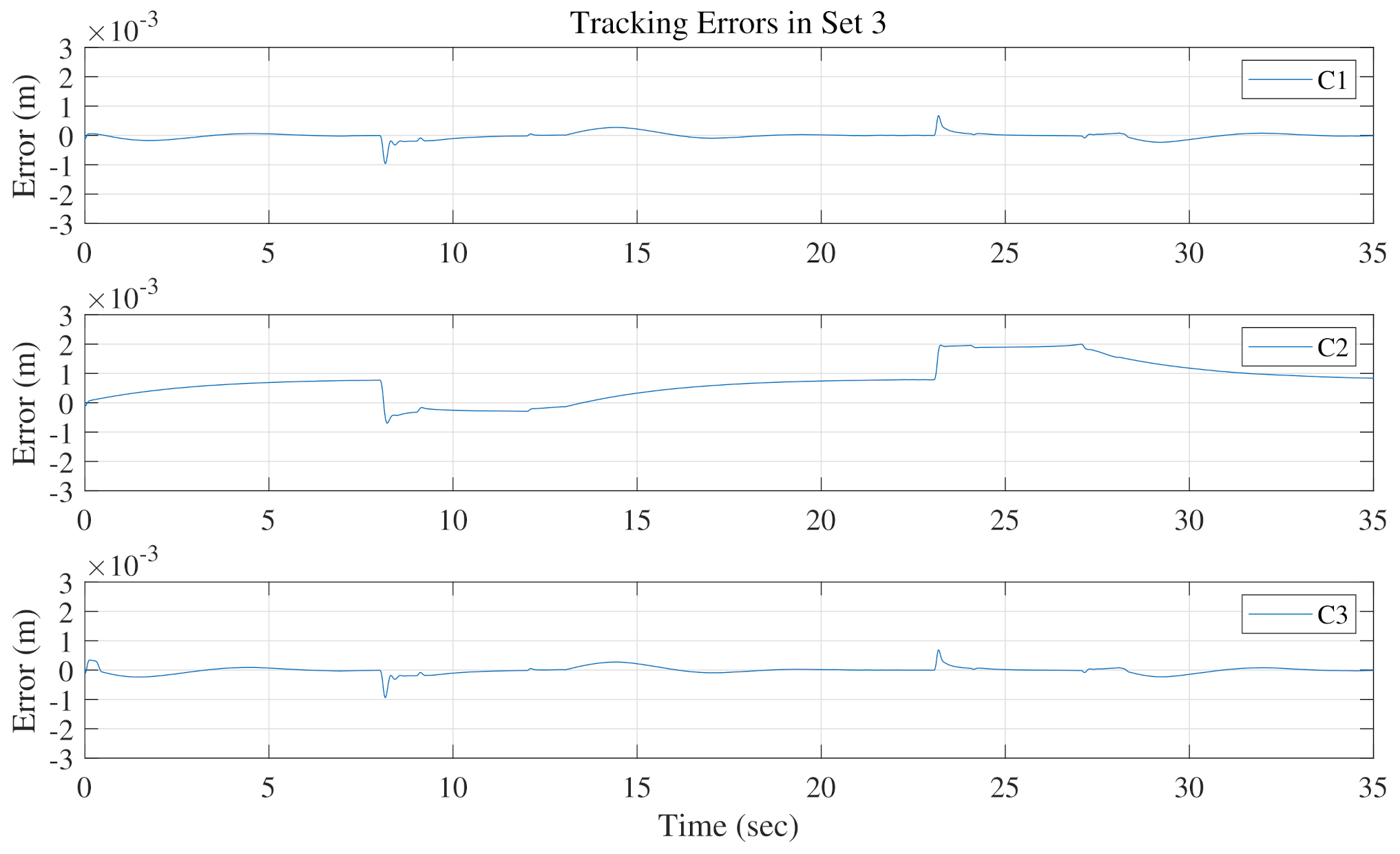
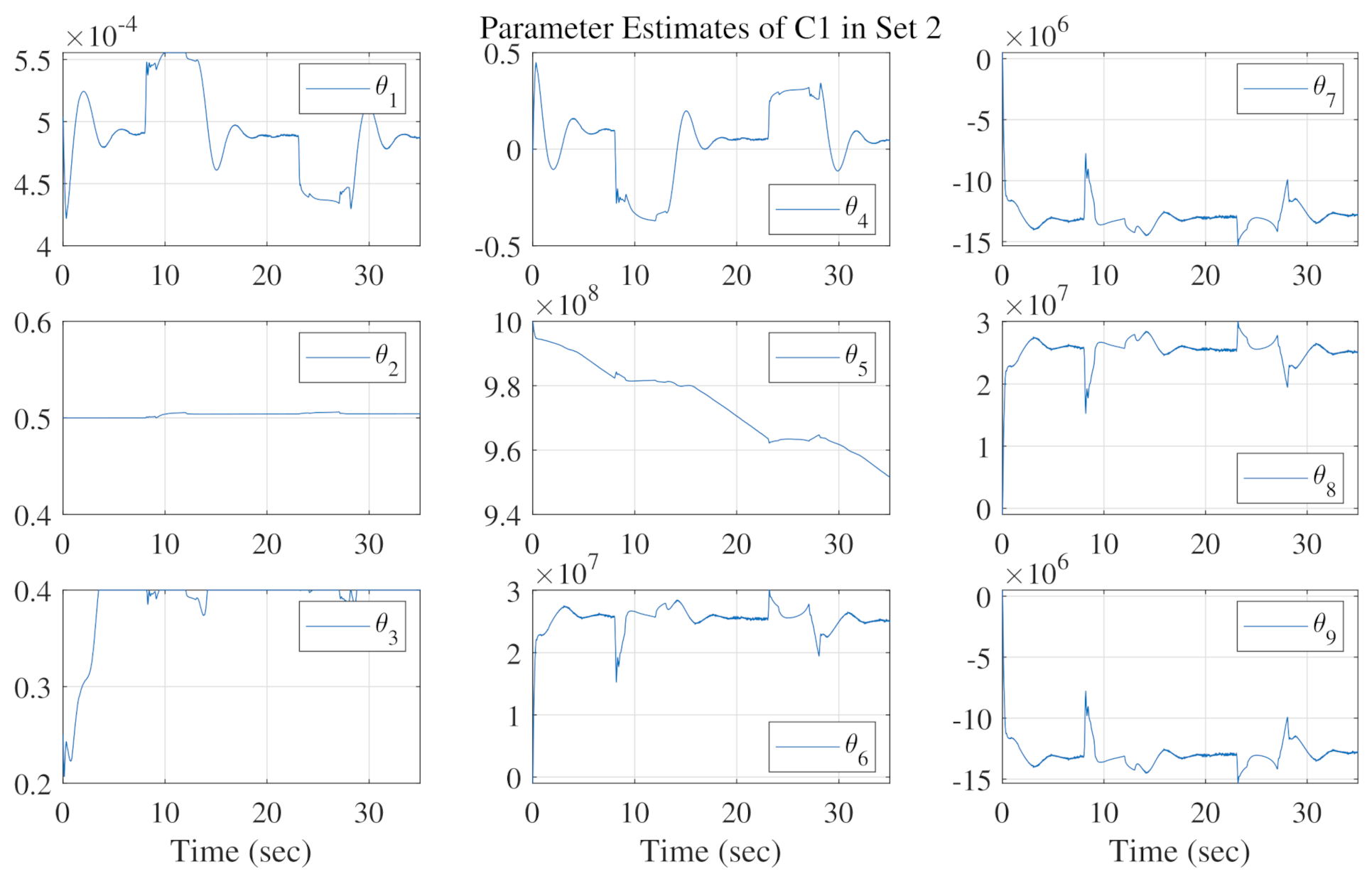
The motion tracking errors of the three control schemes in three sets are shown in Figure 6, Figure 7 and Figure 8, respectively. Comparing C1 with C2, the tracking errors of C1 are much smaller thanks to the effect of parameter adaption. In particular, C1 is able to achieve almost asymptotic tracking performance during the steady state, e.g., when the reference velocity is zero. This is a valuable property, essential for the lifting gantry, since the steady-state tracking error, or the positioning error, is directly related to the quality of segment assembling. The parameter estimation results in three sets are illustrated in Figure 9, Figure 10 and Figure 11, respectively. The parameter estimates change within predetermined ranges and do not show any improper chattering phenomena. In addition, since $F_{c1d}=F_{c2d}=\frac{1}{2}{F}_{Cd}$ is used in C3 to generate the desired cylinder forces, the desired total force $F_{Cd}$ used by the motion tracking controller still can be guaranteed. As expected, the tracking errors of both C1 and C3 in three sets are properly kept within a small range, thanks to the well-designed motion tracking controller for linear motion along the $Y-axis$. To validate the motion tracking performance, the proposed controller C1 achieves a high level of tracking precision, i.e., the midpoint of the crossbeam $y_c$ is able to track the given reference trajectory $y_d\left(t\right)$ with high precision.

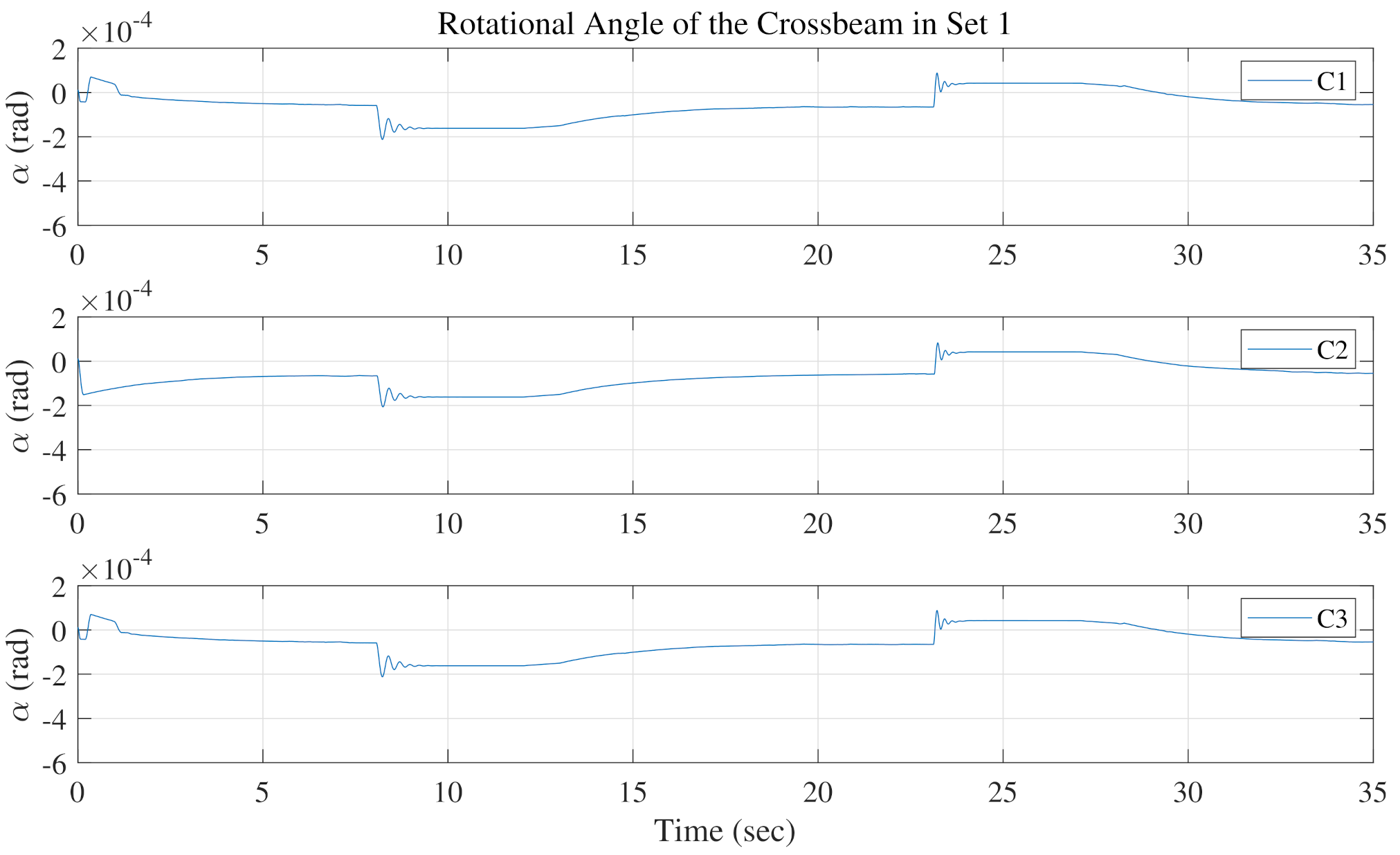
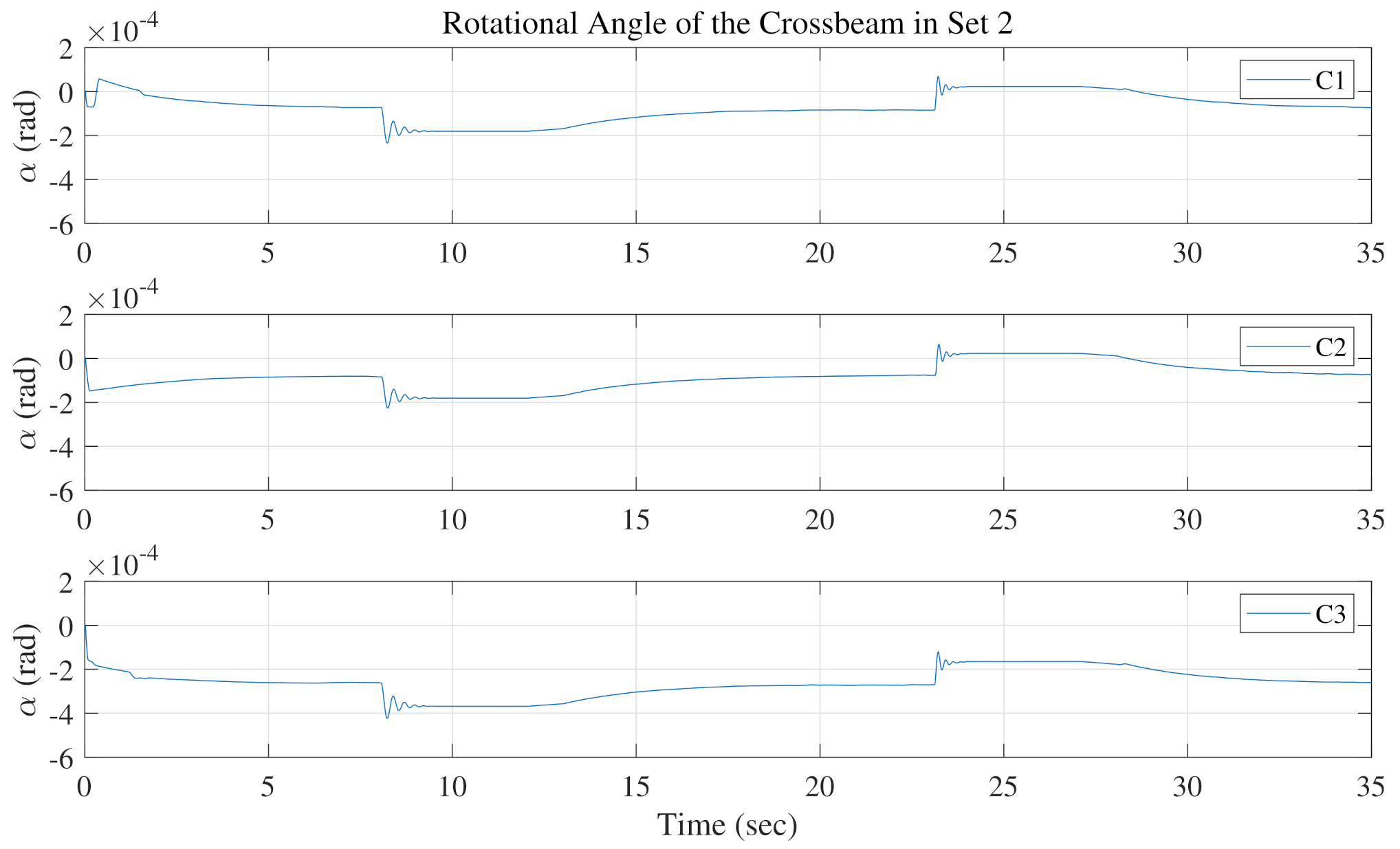
Then, the synchronization performances are compared according to the calculated rotational angle $\alpha$ of the crossbeam. The rotational angles of C1, C2, and C3 in Set 1, where the inclined angle $\Theta$ of the entire lifting gantry is set to zero, are illustrated in Figure 12. Under such ideal working conditions, the loads act equally on the dual cylinders. As expected, the three control schemes are all able to regulate the angles to zero after quick transient processes, and the only difference is that C1 and C2 are slightly quicker. However, when it comes to the unbalanced load conditions, i.e., in Set 2 and Set 3 with the inclined angle $\Theta$ = 0.5 rad, 1 rad, the synchronization performances become distinct, as shown in Figure 13 and Figure 14, respectively. The resulting angles of C1 and C2 are able to converge to very small values after quick transient processes. This comes from the effect of the proposed thrust allocation applied in both C1 and C2. Due to the allocation, the remaining forces pushing the rotational motion, as defined in (17), can be kept small enough, such that the large stiffness of the connections between the crossbeam and guide lines acts as a large proportional feedback to regulate the rotational angle within a very small range. In contrast, without the thrust allocation, the resulting rotational angle of C3 becomes much larger when unbalanced loads act on the dual cylinders. To confirm the synchronization performance, the proposed thrust allocation scheme works well in regulating the unbalanced loads on the dual cylinders and thus leads to a high level of synchronization compared with the commonly used approach.

In summary, according to the comparative simulation results, the proposed control schemes C1 achieves high-precision motion tracking performance and simultaneous high-level synchronization of the dual cylinders in the lifting gantry under unbalanced loads.

5. Conclusions

In this study, the 2-DOF dynamics of the lifting gantry are modeled in detail, where the connections between the crossbeam and guide lines are treated as high-stiffness rotational springs to introduce the additional rotational motion. Then, a model-based synchronization control scheme is developed. Within it, the thrust allocation is designed to regulate the rotational angle to a very small range, and the motion tracking controller is synthesized based on the ARC theory to guarantee the desired motion tracking precision. The theoretical performance is analyzed with detailed proof. Finally, comparative simulations verify the effectiveness of the proposed scheme in dealing with both linear motion tracking and dual-cylinder synchronization. Generally, the study offers a practical control solution for the dual-cylinder mechanisms under unbalanced loads, from complete modeling to control design and validation. In particular, the thrust allocation is easy to implement in practice to achieve high-level synchronization due to its simplicity and independence on precise measurement signals. Therefore, this is a comprehensive study with practical meaning. In future, experiments will be conducted to further validate the performance in a real lifting gantry.

References

- Koyama, Y. Present status and technology of shield tunneling method in Japan. Tunn. Undergr. Space Technol. 2003, 18, 145–159. [Google Scholar] [CrossRef]
- Wang, L.; Gong, G.; Yang, H.; Yang, X.; Hou, D. The development of a high-speed segment erecting system for shield tunneling machine. IEEE/ASME Trans. Mechatron. 2013, 18, 1713–1723. [Google Scholar] [CrossRef]
- Sebbeh-Newton, S.; Ayawah, P.E.; Azure, J.W.; Kaba, A.G.; Ahmad, F.; Zainol, Z.; Zabidi, H. Towards TBM Automation: On-The-Fly Characterization and Classification of Ground Conditions Ahead of a TBM Using Data-Driven Approach. Appl. Sci. 2021, 11, 1060. [Google Scholar] [CrossRef]
- Sun, W.; Shi, M.; Zhang, C.; Zhao, J.; Song, X. Dynamic load prediction of tunnel boring machine (TBM) based on heterogeneous in-situ data. Autom. Constr. 2018, 92, 23–34. [Google Scholar] [CrossRef]
- Gao, X.; Shi, M.; Song, X.; Zhang, C.; Zhang, H. Recurrent neural networks for real-time prediction of TBM operating parameters. Autom. Constr. 2019, 98, 225–235. [Google Scholar] [CrossRef]
- Wang, L.; Sun, W.; Gong, G.; Yang, H. Electro-hydraulic control of high-speed segment erection processes. Autom. Constr. 2017, 73, 67–77. [Google Scholar] [CrossRef]
- Zhou, Y.; Wang, Y.; Ding, L.; Love, P.E. Utilizing IFC for shield segment assembly in underground tunneling. Autom. Constr. 2018, 93, 178–191. [Google Scholar] [CrossRef]
- Zhou, Y.; Luo, H.; Yang, Y. Implementation of augmented reality for segment displacement inspection during tunneling construction. Autom. Constr. 2017, 82, 112–121. [Google Scholar] [CrossRef]
- Yin, F.; Nie, S.; Ji, H.; Huang, Y. Non-probabilistic reliability analysis and design optimization for valve-port plate pair of seawater hydraulic pump for underwater apparatus. Ocean. Eng. 2018, 163, 337–347. [Google Scholar] [CrossRef]
- Lin, T.; Lin, Y.; Ren, H.; Chen, H.; Li, Z.; Chen, Q. A double variable control load sensing system for electric hydraulic excavator. Energy 2021, 223, 119999. [Google Scholar] [CrossRef]
- Ding, R.; Cheng, M.; Zheng, S.; Xu, B. Sensor-Fault-Tolerant Operation for the Independent Metering Control System. IEEE/ASME Trans. Mechatron. 2020. [Google Scholar] [CrossRef]
- Lin, T.; Lin, Y.; Ren, H.; Chen, H.; Chen, Q.; Li, Z. Development and key technologies of pure electric construction machinery. Renew. Sustain. Energy Rev. 2020, 132, 110080. [Google Scholar] [CrossRef]
- Shen, W.; Wang, J. An integral terminal sliding mode control scheme for speed control system using a double-variable hydraulic transformer. ISA Trans. 2019. [Google Scholar] [CrossRef]
- Sun, H.; Chiu, G.C. Motion synchronization for dual-cylinder electrohydraulic lift systems. IEEE/ASME Trans. Mechatron. 2002, 7, 171–181. [Google Scholar]
- Ge, L.; Quan, L.; Zhang, X.; Zhao, B.; Yang, J. Efficiency improvement and evaluation of electric hydraulic excavator with speed and displacement variable pump. Energy Convers. Manag. 2017, 150, 62–71. [Google Scholar] [CrossRef]
- Li, C.; Li, C.; Chen, Z.; Yao, B. Advanced synchronization control of a dual-linear-motor-driven gantry with rotational dynamics. IEEE Trans. Ind. Electron. 2018, 65, 7526–7535. [Google Scholar] [CrossRef]
- Chen, Z.; Li, C.; Yao, B.; Yuan, M.; Yang, C. Integrated coordinated/synchronized contouring control of a dual-linear-motor-driven gantry. IEEE Trans. Ind. Electron. 2019, 67, 3944–3954. [Google Scholar] [CrossRef]
- Zou, S.; Zhao, W. Synchronization and stability control of dual-motor intelligent steer-by-wire vehicle. Mech. Syst. Signal Process. 2020, 145, 106925. [Google Scholar] [CrossRef]
- Li, T.; Yang, T.; Cao, Y.; Xie, R.; Wang, X. Disturbance-estimation based adaptive backstepping fault-tolerant synchronization control for a dual redundant hydraulic actuation system with internal leakage faults. IEEE Access 2019, 7, 73106–73119. [Google Scholar] [CrossRef]
- Yao, B.; Bu, F.; Reedy, J.; Chiu, G.C. Adaptive robust motion control of single-rod hydraulic actuators: Theory and experiments. IEEE/ASME Trans. Mechatron. 2000, 5, 79–91. [Google Scholar]
- Yao, J.; Deng, W. Active Disturbance Rejection Adaptive Control of Hydraulic Servo Systems. IEEE Trans. Ind. Electron. 2017, 64, 8023–8032. [Google Scholar] [CrossRef]
- Guo, Q.; Chen, Z.; Yan, Y.; Jiang, D. Terminal sliding mode velocity control of the electro-hydraulic actuator with lumped uncertainty. Aerosp. Syst. 2021. [Google Scholar] [CrossRef]
- Guo, Q.; Chen, Z. Neural adaptive control of single-rod electrohydraulic system with lumped uncertainty. Mech. Syst. Signal Process. 2021, 146, 106869. [Google Scholar] [CrossRef]
- Lin, F.J.; Chou, P.H.; Chen, C.S.; Lin, Y.S. DSP-based cross-coupled synchronous control for dual linear motors via intelligent complementary sliding mode control. IEEE Trans. Ind. Electron. 2011, 59, 1061–1073. [Google Scholar] [CrossRef]
- Yao, J.; Cao, X.; Zhang, Y.; Li, Y. Cross-coupled fuzzy PID control combined with full decoupling compensation method for double cylinder servo control system. J. Mech. Sci. Technol. 2018, 32, 2261–2271. [Google Scholar] [CrossRef]
- García-Herreros, I.; Kestelyn, X.; Gomand, J.; Coleman, R.; Barre, P.J. Model-based decoupling control method for dual-drive gantry stages: A case study with experimental validations. Control. Eng. Pract. 2013, 21, 298–307. [Google Scholar] [CrossRef] [Green Version]
- Yao, B.; Tomizuka, M. Adaptive robust control of SISO nonlinear systems in a semi-strict feedback form. Automatica 1997, 33, 893–900. [Google Scholar] [CrossRef]
- Yuan, M.; Chen, Z.; Yao, B.; Liu, X. Fast and accurate motion tracking of a linear motor system under kinematic and dynamic constraints: An integrated planning and control approach. IEEE Trans. Control. Syst. Technol. 2021, 29, 804–811. [Google Scholar] [CrossRef]
- Lin, Y.; Chen, Z.; Yao, B. Decoupled torque control of series elastic actuator with adaptive robust compensation of time-varying load-side dynamics. IEEE Trans. Ind. Electron. 2019, 67, 5604–5614. [Google Scholar] [CrossRef]
- Deng, W.; Yao, J. Asymptotic Tracking Control of Mechanical Servosystems with Mismatched Uncertainties. IEEE/ASME Trans. Mechatron. 2020. [Google Scholar] [CrossRef]
- Chen, Z.; Huang, F.; Chen, W.; Zhang, J.; Sun, W.; Chen, J.; Gu, J.; Zhu, S. RBFNN-based adaptive sliding mode control design for delayed nonlinear multilateral telerobotic system with cooperative manipulation. IEEE Trans. Ind. Inform. 2019, 16, 1236–1247. [Google Scholar] [CrossRef]
- Lyu, L.; Chen, Z.; Yao, B. Advanced Valves and Pump Coordinated Hydraulic Control Design to Simultaneously Achieve High Accuracy and High Efficiency. IEEE Trans. Control. Syst. Technol. 2021, 29, 236–248. [Google Scholar] [CrossRef]
- Lyu, L.; Chen, Z.; Yao, B. Development of Pump and Valves Combined Hydraulic System for Both High Tracking Precision and High Energy Efficiency. IEEE Trans. Ind. Electron. 2019, 66, 7189–7198. [Google Scholar] [CrossRef]
- Helian, B.; Chen, Z.; Yao, B. Precision motion control of a servomotor-pump direct-drive electrohydraulic system with a nonlinear pump flow mapping. IEEE Trans. Ind. Electron. 2019, 67, 8638–8648. [Google Scholar] [CrossRef]
- Chen, S.; Han, T.; Dong, F.; Lu, L.; Liu, H.; Tian, X.; Han, J. Precision Interaction Force Control of an Underactuated Hydraulic Stance Leg Exoskeleton Considering the Constraint from the Wearer. Machines 2021, 9, 96. [Google Scholar] [CrossRef]
- Jing, Y.; Pei, W.; Zhaosheng, D.; JIANG, D.; Tong, S. A novel architecture of electro-hydrostatic actuator with digital distribution. Chin. J. Aeronaut. 2021, 34, 224–238. [Google Scholar]
Figure 1.
Background about the segment erector in a shield tunneling machine in practice. (a) General structures of a tunnel and a shield tunneling machine. (b) A segment erector in practical engineering. (c) The typical structure of a segment erector. This study focuses on the dual-cylinder lifting gantry in the segment erector. The lifting gantry usually works at an inclined angle, which leads to unbalanced loads on the two sides.
Figure 2.
Simplified structure of a typical segment erector at an inclined angle.
Figure 3.
Schematic diagram of the dual-cylinder lifting gantry at a certain rotational angle of . (a) General configuration of the lifting gantry. (b) Linear and rotational motions of the lifting gantry.
Figure 4.
Synchronization controller structure.
Figure 5.
Reference trajectory used in simulation.
Figure 6.
Motion tracking errors comparison in Set 1.
Figure 7.
Motion tracking errors comparison in Set 2.
Figure 8.
Motion tracking errors comparison in Set 3.
Figure 9.
Parameter estimation results of C1 in Set 1.
Figure 10.
Parameter estimation results of C1 in Set 2.
Figure 11.
Parameter estimation results of C1 in Set 3.
Figure 12.
Rotational angles comparison in Set 1.
Figure 13.
Rotational angles comparison in Set 2.
Figure 14.
Rotational angles comparison in Set 3.
Publisher’s Note: MDPI stays neutral with regard to jurisdictional claims in published maps and institutional affiliations. |
© 2021 by the authors. Licensee MDPI, Basel, Switzerland. This article is an open access article distributed under the terms and conditions of the Creative Commons Attribution (CC BY) license (https://creativecommons.org/licenses/by/4.0/).
Share and Cite
MDPI and ACS Style
Lyu, L.; Liang, X.; Guo, J. Synchronization Control of a Dual-Cylinder Lifting Gantry of Segment Erector in Shield Tunneling Machine under Unbalance Loads. Machines 2021, 9, 152. https://0-doi-org.brum.beds.ac.uk/10.3390/machines9080152
AMA Style
Lyu L, Liang X, Guo J. Synchronization Control of a Dual-Cylinder Lifting Gantry of Segment Erector in Shield Tunneling Machine under Unbalance Loads. Machines. 2021; 9(8):152. https://0-doi-org.brum.beds.ac.uk/10.3390/machines9080152
Chicago/Turabian StyleLyu, Litong, Xiao Liang, and Jingbo Guo. 2021. "Synchronization Control of a Dual-Cylinder Lifting Gantry of Segment Erector in Shield Tunneling Machine under Unbalance Loads" Machines 9, no. 8: 152. https://0-doi-org.brum.beds.ac.uk/10.3390/machines9080152
Note that from the first issue of 2016, this journal uses article numbers instead of page numbers. See further details here.