
Application of Artificial Intelligence in the MRI Classification Task of Human Brain Neurological and Psychiatric Diseases: A Scoping Review

Abstract
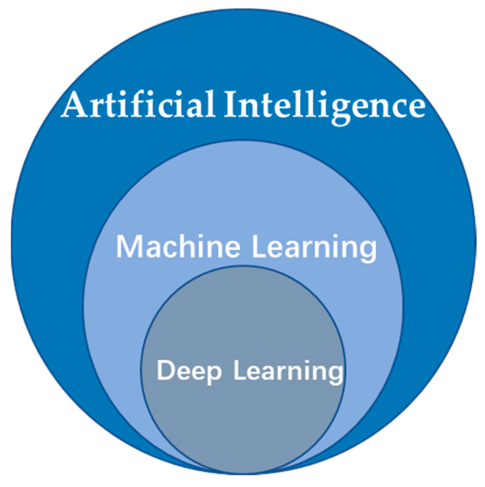
:1. Introduction
2. Methods
2.1. Search Strategy and Literature Sources
2.2. Inclusion Criteria
2.3. Exclusion Criteria
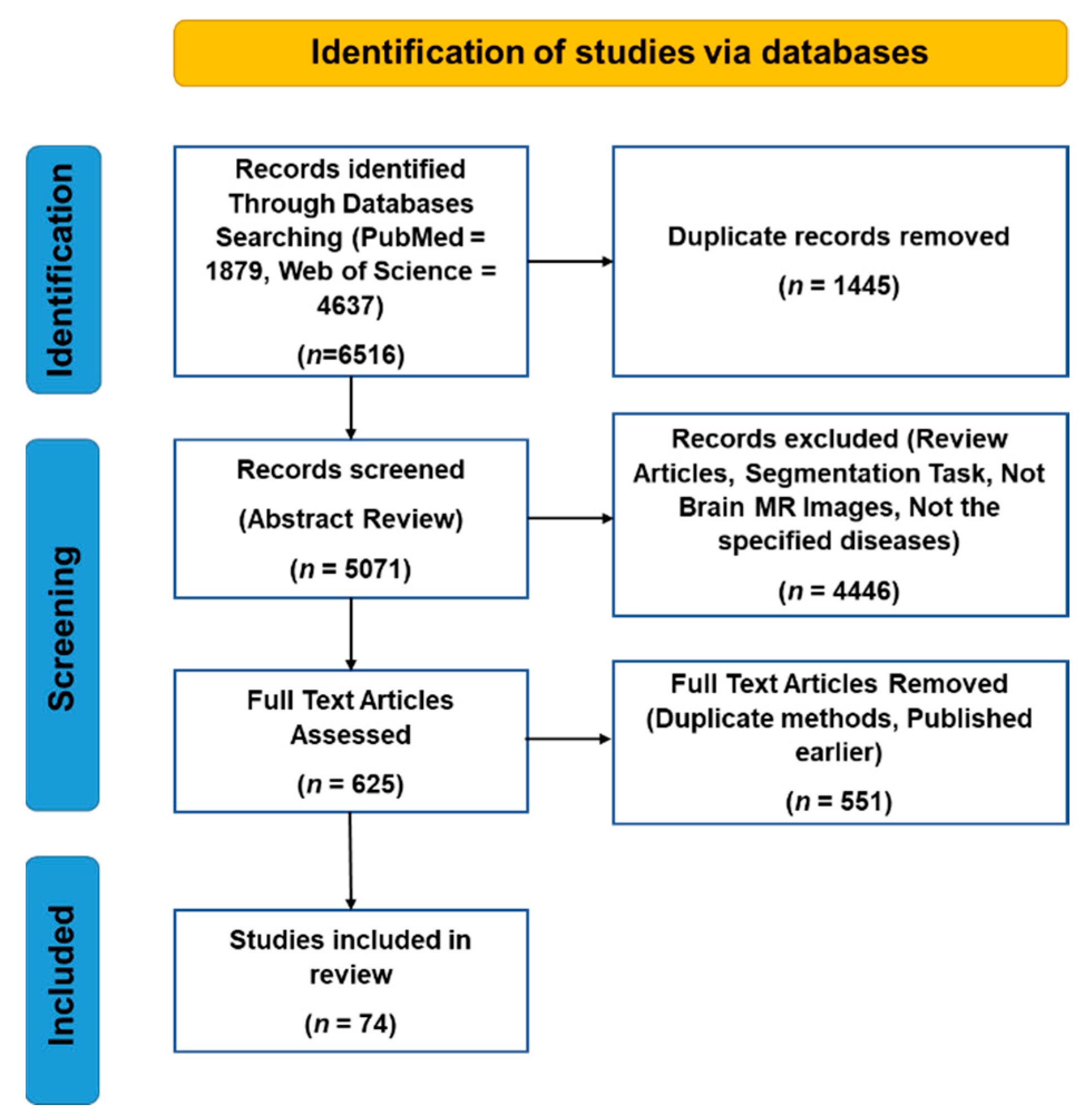
2.4. Results
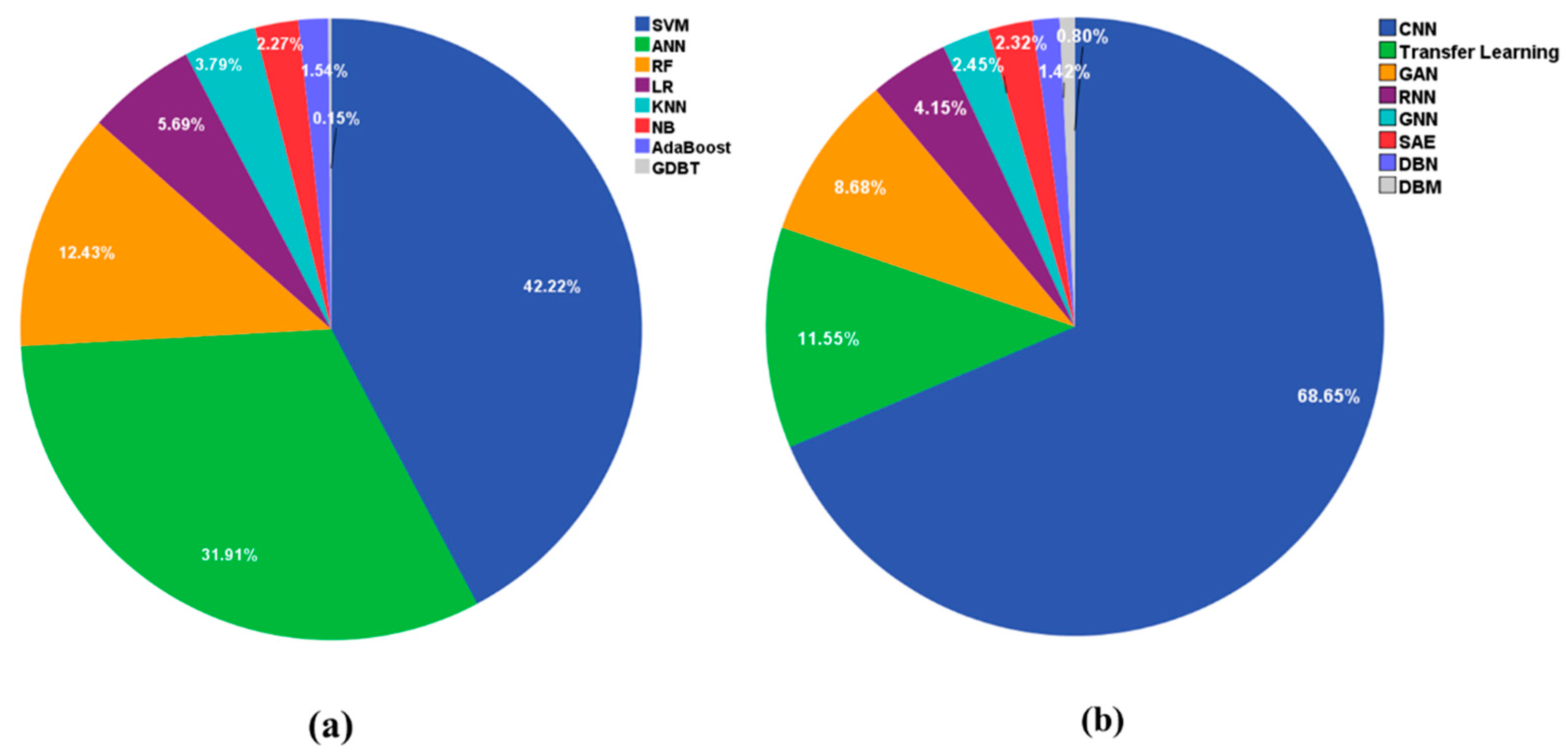
3. Related Machine Learning Methods
3.1. K-Nearest Neighbor (KNN)
3.2. Naive Bayes (NB)
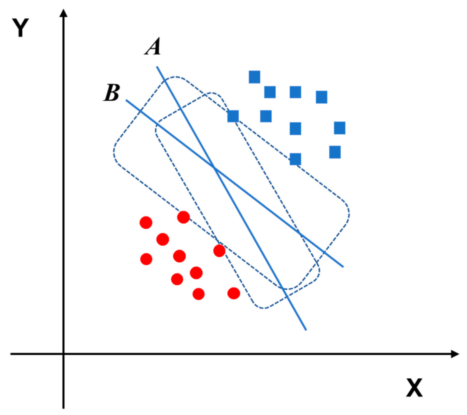
3.3. Support Vector Machine (SVM)
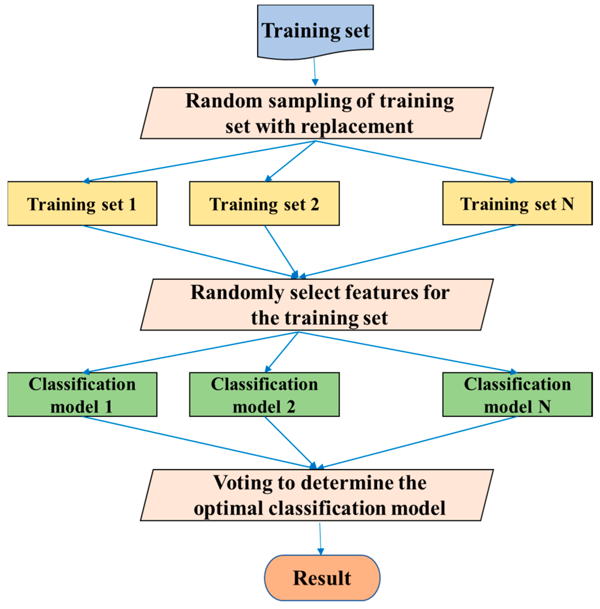
3.4. Random Forests (RF)
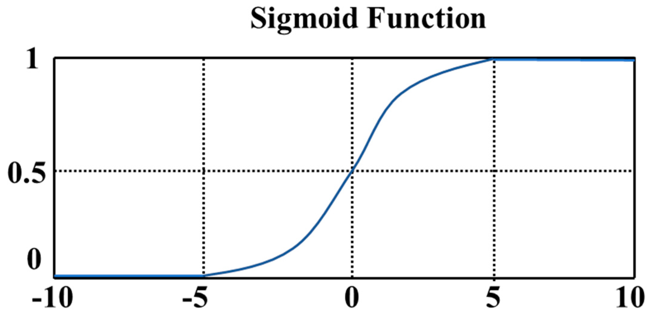
3.5. Logistic Regression (LR)
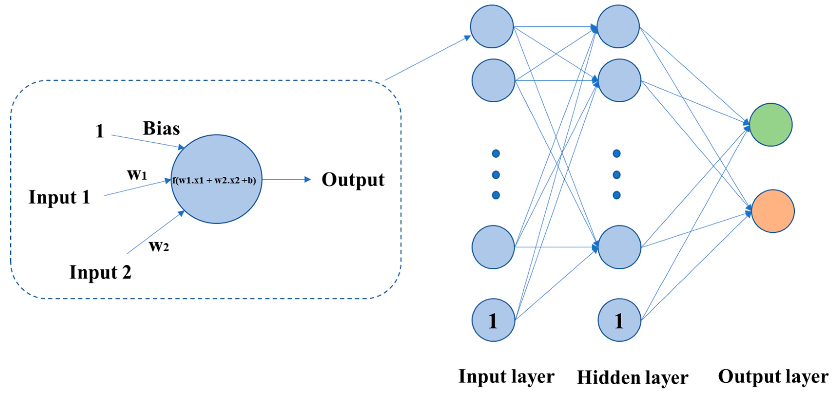
3.6. Artificial Neural Network (ANN)
4. Related Deep Learning Methods
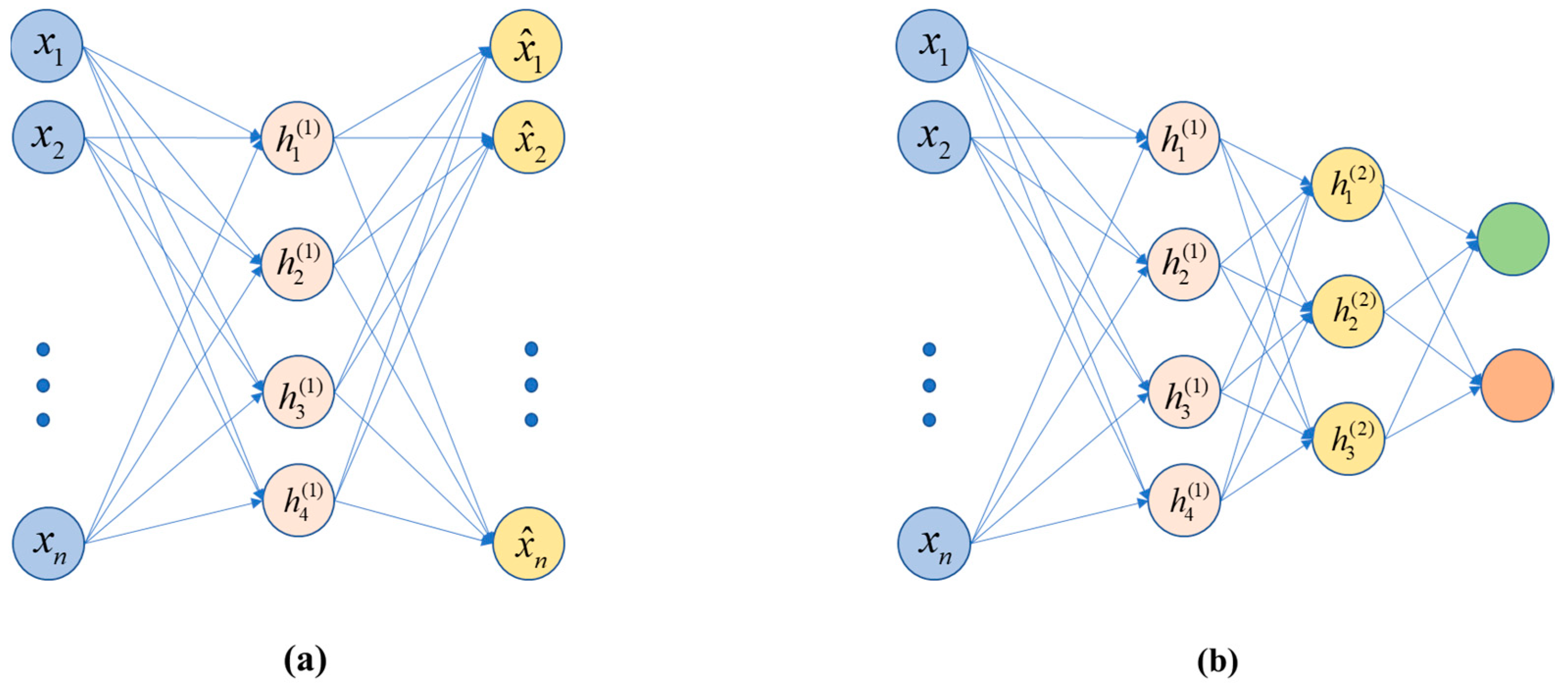
4.1. Stacked Auto-Encoders (SAE)
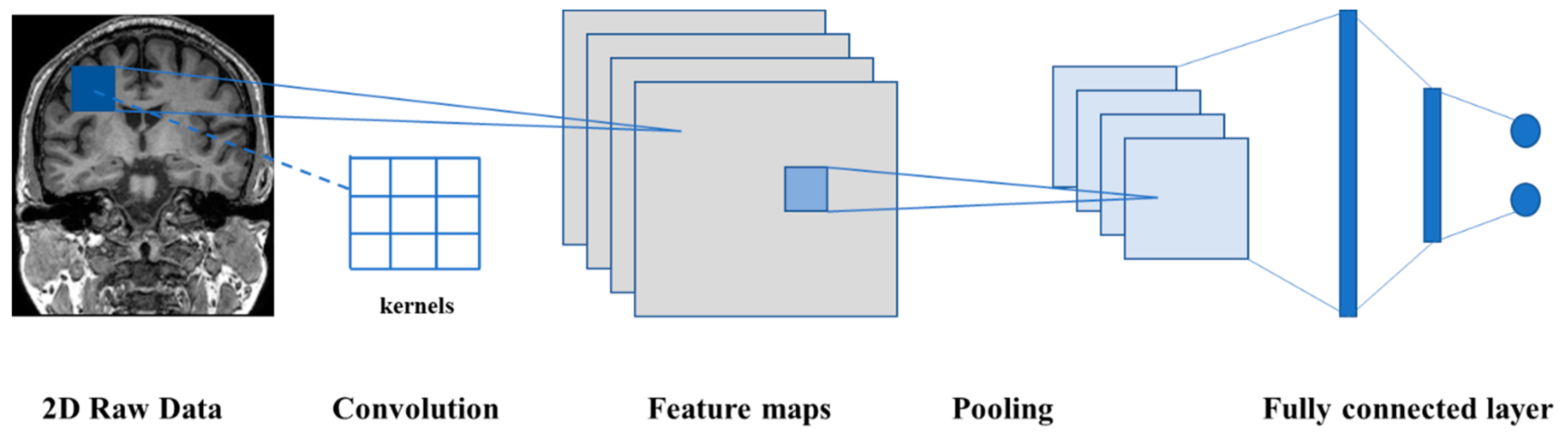
4.2. D Convolutional Neural Network (2D-CNN)
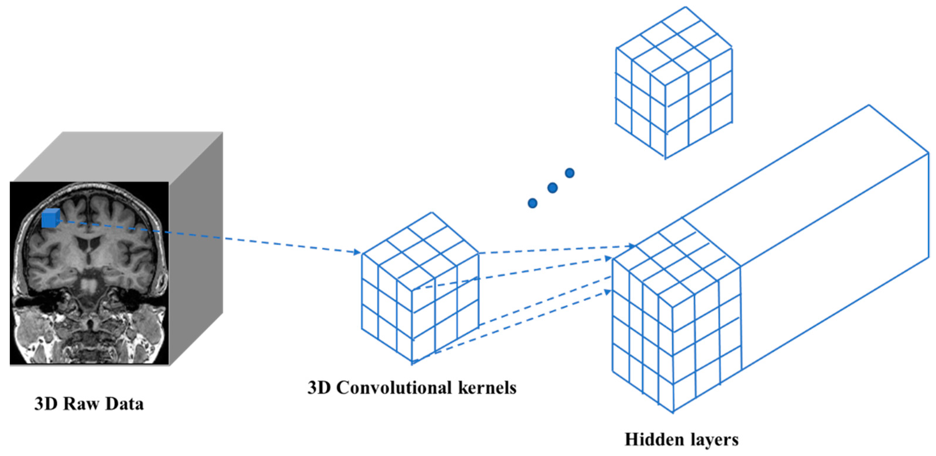
4.3. D Convolutional Neural Network (3D-CNN)
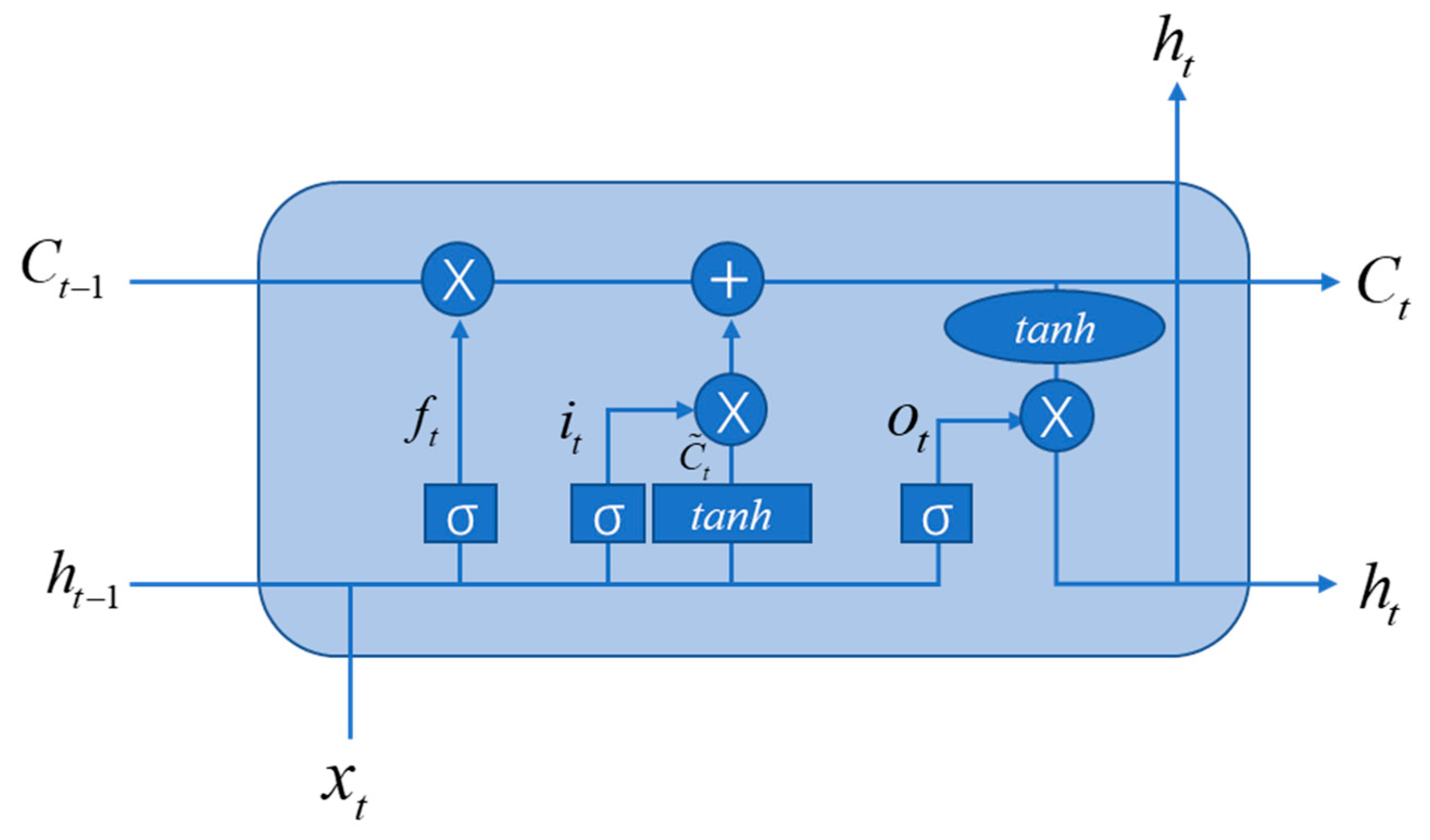
4.4. Recurrent Neural Network (RNN)
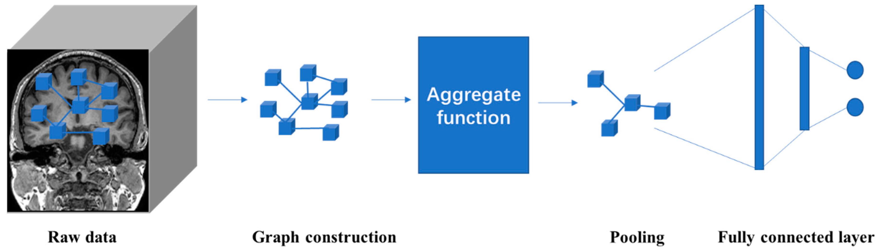
4.5. Graph Neural Network (GNN)
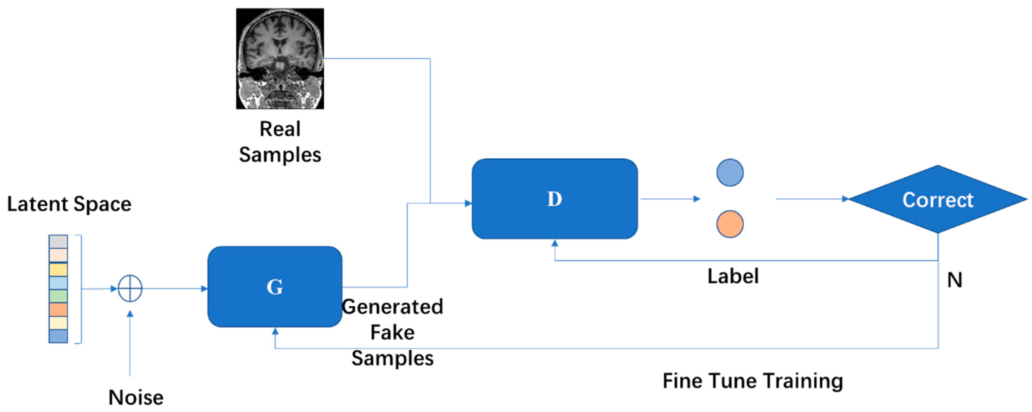
4.6. Generative Adversarial Network (GAN)
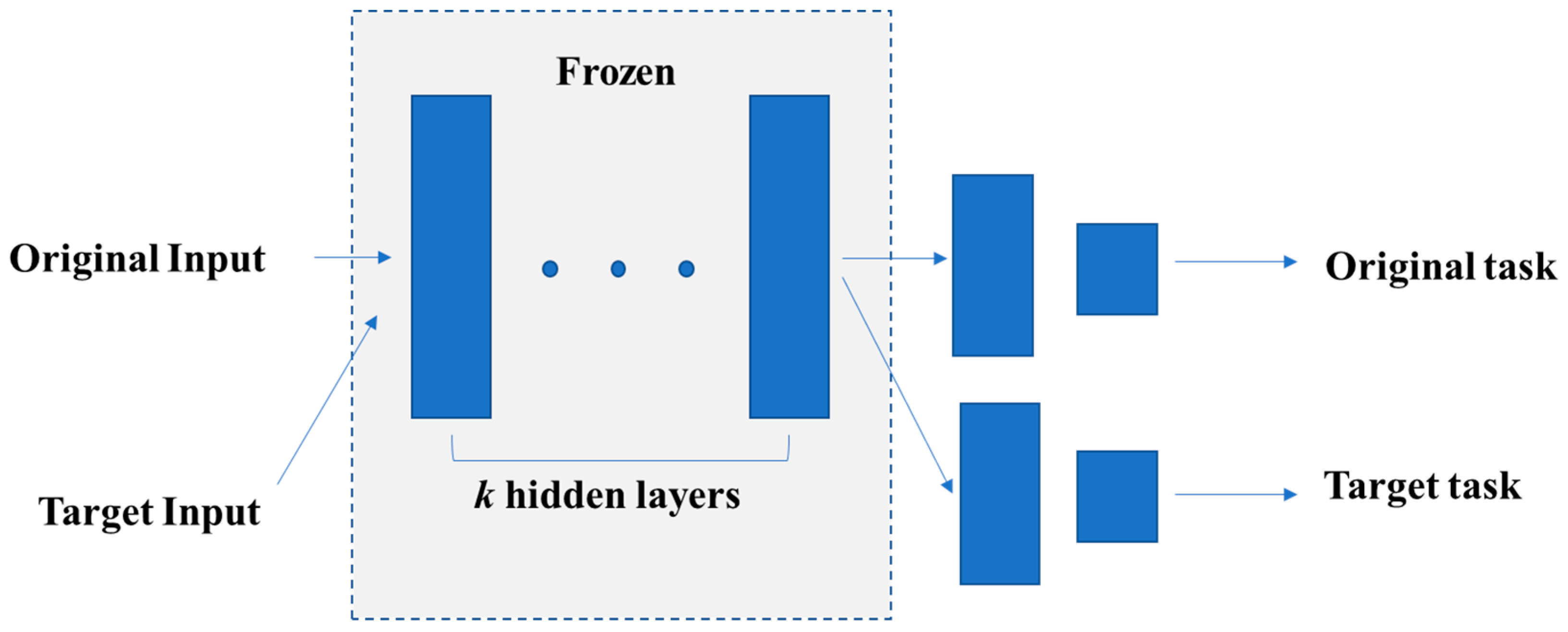
4.7. Transfer Learning
5. Applications in Human Brain MRI Image Classification Tasks
5.1. Alzheimer’s Disease
5.2. Parkinson’s Disease
5.3. Major Depressive Disorder
5.4. Schizophrenia
5.5. Attention-Deficit/Hyperactivity Disorder
5.6. Autism Spectrum Disorder
6. Conclusions and Discussion
Author Contributions
Funding
Conflicts of Interest
References
- Brody, H. Medical imaging. Nat. Cell Biol. 2013, 502, S81. [Google Scholar] [CrossRef]
- Yousaf, T.; Dervenoulas, G.; Politis, M. Chapter Two-Advances in MRI Methodology. In International Review of Neurobiology; Politis, M., Ed.; Academic Press: Cambridge, MA, USA, 2018; Volume 141, pp. 31–76. [Google Scholar]
- Akhavan Aghdam, M.; Sharifi, A.; Pedram, M.M. Combination of rs-fMRI and sMRI Data to Discriminate Autism Spectrum Disorders in Young Children Using Deep Belief Network. J. Digit. Imaging 2018, 31, 895–903. [Google Scholar] [CrossRef]
- Currie, G.; Hawk, K.E.; Rohren, E.; Vial, A.; Klein, R. Machine Learning and Deep Learning in Medical Imaging: Intelligent Imaging. J. Med. Imaging Radiat. Sci. 2019, 50, 477–487. [Google Scholar] [CrossRef] [Green Version]
- Shavlik, J.; Dietterich, T. Readings in Machine Learning; San Mateo Morgan Kaufmann: Burlington, MA, USA, 1990. [Google Scholar]
- Michie, D.; Spiegelhalter, D.; Taylor, C. Machine Learning, Neural and Statistical Classification. Technometrics 1999, 37, 459. [Google Scholar] [CrossRef]
- Erickson, B.J.; Korfiatis, P.; Akkus, Z.; Kline, T.L. Machine Learning for Medical Imaging. Radiographics 2017, 37, 505–515. [Google Scholar] [CrossRef]
- LeCun, Y.; Bengio, Y.; Hinton, G. Deep learning. Nature 2015, 521, 436–444. [Google Scholar] [CrossRef] [PubMed]
- Schmidhuber, J. Deep learning in neural networks: An overview. Neural Netw. 2015, 61, 85–117. [Google Scholar] [CrossRef] [PubMed] [Green Version]
- Noor, M.B.T.; Zenia, N.Z.; Kaiser, M.S.; Al Mamun, S.; Mahmud, M. Application of deep learning in detecting neurological disorders from magnetic resonance images: A survey on the detection of Alzheimer’s disease, Parkinson’s disease and schizophrenia. Brain Inform. 2020, 7, 1–21. [Google Scholar] [CrossRef] [PubMed]
- Mahmud, M.; Kaiser, M.; Hussain, A.; Vassanelli, S. Applications of Deep Learning and Reinforcement Learning to BiologicalData. IEEE Trans. Neural Netw. Learn Syst. 2018, 29, 2063–2079. [Google Scholar] [CrossRef] [Green Version]
- Mahmud, M.; Kaiser, M.S.; McGinnity, T.M.; Hussain, A. Deep Learning in Mining Biological Data. Cogn. Comput. 2021, 13, 1–33. [Google Scholar] [CrossRef]
- Jo, T.; Nho, K.; Saykin, A.J. Deep Learning in Alzheimer’s Disease: Diagnostic Classification and Prognostic Prediction Using Neuroimaging Data. Front. Aging Neurosci. 2019, 11, 220. [Google Scholar] [CrossRef] [Green Version]
- Vasquez-Correa, J.C.; Arias-Vergara, T.; Orozco-Arroyave, J.R.; Eskofier, B.M.; Klucken, J.; Noth, E. Multimodal Assessment of Parkinson’s Disease: A Deep Learning Approach. IEEE J. Biomed. Health Inform. 2019, 23, 1618–1630. [Google Scholar] [CrossRef]
- Uyulan, C.; Ergüzel, T.T.; Unubol, H.; Cebi, M.; Sayar, G.H.; Asad, M.N.; Tarhan, N. Major Depressive Disorder Classification Based on Different Convolutional Neural Network Models: Deep Learning Approach. Clin. EEG Neurosci. 2021, 52, 38–51. [Google Scholar] [CrossRef] [PubMed]
- Oh, J.; Oh, B.-L.; Lee, K.-U.; Chae, J.-H.; Yun, K. Identifying Schizophrenia Using Structural MRI with a Deep Learning Algorithm. Front. Psychiatry 2020, 11, 16. [Google Scholar] [CrossRef] [PubMed]
- Du, Y.; Fu, Z.; Calhoun, V.D. Classification and Prediction of Brain Disorders Using Functional Connectivity: Promising but Challenging. Front. Neurosci. 2018, 12, 525. [Google Scholar] [CrossRef]
- Lord, C.; Elsabbagh, M.; Baird, G.; Veenstra-Vanderweele, J. Autism spectrum disorder. Lancet 2018, 392, 508–520. [Google Scholar] [CrossRef]
- Hosseini, M.-P.; Tran, T.X.; Pompili, D.; Elisevich, K.; Soltanian-Zadeh, H. Multimodal data analysis of epileptic EEG and rs-fMRI via deep learning and edge computing. Artif. Intell. Med. 2020, 104, 101813. [Google Scholar] [CrossRef] [PubMed]
- Mazurowski, M.A.; Buda, M.; Saha, A.; Bashir, M.R. Deep learning in radiology: An overview of the concepts and a survey of the state of the art with focus on MRI. JMRI 2019, 49, 939–954. [Google Scholar] [CrossRef]
- Hu, Z.; Tang, J.; Wang, Z.; Zhang, K.; Zhang, L.; Sun, Q. Deep learning for image-based cancer detection and diagnosis−A survey. Pattern Recognit. 2018, 83, 134–149. [Google Scholar] [CrossRef]
- Segato, A.; Marzullo, A.; Calimeri, F.; De Momi, E. Artificial intelligence for brain diseases: A systematic review. APL Bioeng. 2020, 4, 041503. [Google Scholar] [CrossRef]
- Zhang, L.; Wang, M.; Liu, M.; Zhang, D. A Survey on Deep Learning for Neuroimaging-Based Brain Disorder Analysis. Front. Neurosci. 2020, 14, 779. [Google Scholar] [CrossRef]
- Lundervold, A.; Lundervold, A. An overview of deep learning in medical imaging focusing on MRI. Z. Med. Phys. 2019, 29, 102–127. [Google Scholar] [CrossRef]
- Steardo, L.; Carbone, E.A.; de Filippis, R.; Pisanu, C.; Segura-Garcia, C.; Squassina, A.; De Fazio, P. Application of Support Vector Machine on fMRI Data as Biomarkers in Schizophrenia Diagnosis: A Systematic Review. Front. Psychiatry 2020, 11, 588. [Google Scholar] [CrossRef]
- Litjens, G.; Kooi, T.; Bejnordi, B.E.; Setio, A.A.A.; Ciompi, F.; Ghafoorian, M.; van der Laak, J.A.; van Ginneken, B.; Sánchez, C.I. A survey on deep learning in medical image analysis. Med. Image Anal. 2017, 42, 60–88. [Google Scholar] [CrossRef] [PubMed] [Green Version]
- Durstewitz, D.; Koppe, G.; Meyer-Lindenberg, A. Deep neural networks in psychiatry. Mol. Psychiatry 2019, 24, 1583–1598. [Google Scholar] [CrossRef] [PubMed]
- Arskey, H.; O’Malley, L. Scoping studies: Towards a methodological framework. Int. J. Soc. Res. Methodol. 2005, 8, 19–32. [Google Scholar]
- Tricco, A.C.; Lillie, E.; Zarin, W.; O’Brien, K.K.; Colquhoun, H.; Levac, D.; Moher, D.; Peters, M.D.J.; Horsley, T.; Weeks, L.; et al. PRISMA Extension for Scoping Reviews (PRISMA-ScR): Checklist and Explanation. Ann. Intern. Med. 2018, 169, 467–473. [Google Scholar] [CrossRef] [PubMed] [Green Version]
- Peters, M.D.J.; Marnie, C.; Tricco, A.C.; Pollock, D.; Munn, Z.; Alexander, L.; McInerney, P.; Godfrey, C.M.; Khalil, H. Updated methodological guidance for the conduct of scoping reviews. JBI Evid. Synth. 2020, 18, 2119–2126. [Google Scholar] [CrossRef] [PubMed]
- Peterson, L.E. K-nearest neighbor. Scholarpedia 2009, 4, 1883. [Google Scholar] [CrossRef]
- Weinberger, K.Q. Distance Metric Learning for Large Margin Nearest Neighbor Classification. JMLR 2009, 10, 207–244. [Google Scholar]
- Rish, I. An Empirical Study of the Naïve Bayes Classifier. In Proceedings of the IJCAI 2001 Workshop on Empirical Methods in Artificial Intelligence, Seattle, WA, USA, 4 August 2001; Volume 3, pp. 41–46. [Google Scholar]
- Battineni, G.; Sagaro, G.G.; Nalini, C.; Amenta, F.; Tayebati, S.K. Comparative Machine-Learning Approach: A Follow-Up Study on Type 2 Diabetes Predictions by Cross-Validation Methods. Mach Lear 2019, 7, 74. [Google Scholar] [CrossRef] [Green Version]
- Campbell, C.; Ying, Y. Learning with Support Vector Machines. Synth. Lect. Artif. Intell. Mach. Learn. 2011, 5, 1–95. [Google Scholar] [CrossRef]
- Lee, L.H.; Wan, C.H.; Rajkumar, R.; Isa, D. An enhanced Support Vector Machine classification framework by using Euclidean distance function for text document categorization. Appl. Intell. 2012, 37, 80–99. [Google Scholar] [CrossRef]
- Zhou, J.; Shi, J.; Li, G. Fine tuning support vector machines for short-term wind speed forecasting. Energy Convers. Manag. 2011, 52, 1990–1998. [Google Scholar] [CrossRef]
- Breiman, L. Random Forests. Mach. Learn. 2001, 45, 5–32. [Google Scholar] [CrossRef] [Green Version]
- Breiman, L. Bagging predictors. Mach. Learn. 1996, 24, 123–140. [Google Scholar] [CrossRef] [Green Version]
- Cornfield, J.; Gordon, T.; Smith, W. Quantal Response Curves for Experimentally Uncontrolled Variables. Bull. Int. Stat. Inst. 1961, 38, 97–115. [Google Scholar]
- Domínguez-Almendros, S.; Benítez-Parejo, N.; Gonzalez-Ramirez, A.R. Logistic regression models. Allergol. Immunopathol. 2011, 39, 295–305. [Google Scholar] [CrossRef]
- Vincent, P.; LaRochelle, H.; Bengio, Y.; Manzagol, P.-A. Extracting and composing robust features with denoising autoencoders. In Proceedings of the ICML 2008, Montreal, QC, Canada, 11–15 April 2016; pp. 1096–1103. [Google Scholar]
- Poultney, C.S.; Chopra, S.; Cun, Y.L. Efficient Learning of Sparse Representations with An Energy-based Model. Adv. Neural Inf. Process. Syst. 2007, 19, 1137. [Google Scholar]
- Kingma, D.; Welling, M. Auto-Encoding Variational Bayes. In Proceedings of the ICLR, Banff, AB, Canada, 14–16 April 2014. [Google Scholar]
- LeCun, Y.; Bottou, L.; Bengio, Y.; Haffner, P. Gradient-based learning applied to document recognition. Proc. IEEE 1998, 86, 2278–2324. [Google Scholar] [CrossRef] [Green Version]
- Ganapathy, N.; Swaminathan, R.; Deserno, T.M. Deep Learning on 1-D Biosignals: A Taxonomy-based Survey. Yearb. Med. Inform. 2018, 27, 98–109. [Google Scholar] [CrossRef] [Green Version]
- Ji, S.; Xu, W.; Yang, M.; Yu, K. 3D Convolutional Neural Networks for Human Action Recognition. IEEE Trans. Pattern Anal. Mach. Intell. 2013, 35, 221–231. [Google Scholar] [CrossRef] [Green Version]
- Gao, X.W.; Hui, R.; Tian, Z. Classification of CT brain images based on deep learning networks. Comput. Methods Programs Biomed. 2017, 138, 49–56. [Google Scholar] [CrossRef] [PubMed] [Green Version]
- Hüsken, M.; Stagge, P. Recurrent neural networks for time series classification. Neurocomputing 2003, 50, 223–235. [Google Scholar] [CrossRef]
- Hopfield, J.J. Neural networks and physical systems with emergent collective computational abilities. Proc. Natl. Acad. Sci. USA 1982, 79, 2554–2558. [Google Scholar] [CrossRef] [PubMed] [Green Version]
- Gonzalez, R.; Riascos Salas, J.; Barone, D.; Andres, J. How Artificial Intelligence is Supporting Neuroscience Research: A Discussion About Foundations, Methods and Applications. In Proceedings of the Latin American Workshop on Computational Neuroscience, Porto Alegre, Brazil, 22–24 November 2017; pp. 63–77. [Google Scholar]
- Barak, O. Recurrent neural networks as versatile tools of neuroscience research. Curr. Opin. Neurobiol. 2017, 46, 1–6. [Google Scholar] [CrossRef]
- Güçlü, U.; van Gerven, M.A.J. Modeling the Dynamics of Human Brain Activity with Recurrent Neural Networks. Front. Comput. Neurosci. 2017, 11, 7. [Google Scholar] [CrossRef] [Green Version]
- Hochreiter, S.; Schmidhuber, J. Long short-term memory. Neural Comput. 1997, 9, 1735–1780. [Google Scholar] [CrossRef]
- Sperduti, A.; Starita, A. Supervised neural networks for the classification of structures. IEEE Trans. Neural Netw. 1997, 8, 714–735. [Google Scholar] [CrossRef] [Green Version]
- Gori, M.; Monfardini, G.; Scarselli, F. A New Model for Learning in Graph Domains. In Proceedings of the 2005 IEEE International Joint Conference on Neural Networks, Montreal, QC, Canada, 31 July–4 August 2005; Volume 722, pp. 729–734. [Google Scholar]
- Scarselli, F.; Gori, M.; Tsoi, A.C.; Hagenbuchner, M.; Monfardini, G. The Graph Neural Network Model. IEEE Trans. Neural Netw. 2009, 20, 61–80. [Google Scholar] [CrossRef] [Green Version]
- Gallicchio, C.; Micheli, A. Graph Echo State Networks. In Proceedings of the Neural Networks (IJCNN), Barcelona, Spain, 18–23 July 2010; pp. 1–8. [Google Scholar]
- Li, Y.; Tarlow, D.; Brockschmidt, M.; Zemel, R. Gated Graph Sequence Neural Networks. arXiv 2015, arXiv:1511.05493. [Google Scholar]
- Dai, H.; Kozareva, Z.; Dai, B.; Smola, A.; Song, L. Learning Steady-States of Iterative Algorithms Over Graphs. In Proceedings of the 35th International Conference on Machine Learning, Proceedings of Machine Learning Research, Stockholm, Sweden, 10–15 July 2018; pp. 1106–1114. [Google Scholar]
- Perozzi, B.; Al-Rfou, R.; Skiena, S. DeepWalk: Online Learning of Social Representations. In Proceedings of the 20th ACM SIGKDD International Conference on Knowledge Discovery and Data Mining, New York, NY, USA, 24–27 August 2014; pp. 701–710. [Google Scholar] [CrossRef] [Green Version]
- Kipf, T.N.; Welling, M. Semi-Supervised Classification with Graph Convolutional Networks. In Proceedings of the ICLR 2017, Toulon, France, 24–26 April 2017. [Google Scholar]
- Nguyen, G.; Lee, J.; Rossi, R.; Ahmed, N.; Koh, E.; Kim, S. Continuous-Time Dynamic Network Embeddings. In Proceedings of the Companion of the The Web Conference 2018, Lyon, France, 23–27 April 2018; pp. 969–976. [Google Scholar]
- Kumar, S.; Zhang, X.; Leskovec, J. Predicting Dynamic Embedding Trajectory in Temporal Interaction Networks. In Proceedings of the 25th ACM SIGKDD International Conference on Knowledge Discovery and Data Mining, Anchorage, AK, USA, 4–8 August 2019; pp. 1269–1278. [Google Scholar]
- Goodfellow, I.; Pouget-Abadie, J.; Mirza, M.; Xu, B.; Warde-Farley, D.; Ozair, S.; Courville, A.; Bengio, Y. Generative Adversarial Nets. arXiv 2014, arXiv:1406.2661. [Google Scholar]
- Creswell, A.; White, T.; Dumoulin, V.; Arulkumaran, K.; Sengupta, B.; Bharath, A.A. Generative Adversarial Networks: An Overview. IEEE Signal Process. Mag. 2018, 35, 53–65. [Google Scholar] [CrossRef] [Green Version]
- Hong, Y.; Hwang, U.; Yoo, J.; Yoon, S. How Generative Adversarial Networks and Their Variants Work. ACM Comput. Surv. 2019, 52, 1–43. [Google Scholar] [CrossRef] [Green Version]
- Guo, Y.; Liu, Y.; Oerlemans, A.; Lao, S.; Wu, S.; Lew, M.S. Deep learning for visual understanding: A review. Neurocomputing 2016, 187, 27–48. [Google Scholar] [CrossRef]
- Lan, L.; You, L.; Zhang, Z.; Fan, Z.; Zhao, W.; Zeng, N.; Chen, Y.; Zhou, X. Generative Adversarial Networks and Its Applications in Biomedical Informatics. Front. Public Health 2020, 8, 164. [Google Scholar] [CrossRef] [PubMed]
- Mensch, A.; Mairal, J.; Bzdok, D.; Thirion, B.; Varoquaux, G. Learning Neural Representations of Human Cognition Across Many fMRI Studies. In Proceedings of the NIPS 2017, Long Beach, CA, USA, 4–9 December 2017. [Google Scholar]
- Oord, A.; Li, Y.; Vinyals, O. Representation Learning with Contrastive Predictive Coding. arXiv 2018, arXiv:1807.03748. [Google Scholar]
- Thomas, A.W.; Müller, K.-R.; Samek, W. Deep Transfer Learning for Whole-Brain FMRI Analyses. Trans. Petri Nets Other Models Concurr. XV 2019, 59–67. [Google Scholar] [CrossRef] [Green Version]
- Yosinski, J.; Clune, J.; Bengio, Y.; Lipson, H. How Transferable Are Features in Deep Neural Networks? In Proceedings of the Advances in Neural Information Processing Systems (NIPS) 2014, Montreal, QC, Canada, 8–13 December 2014. [Google Scholar]
- Burns, A.; Iliffe, S. Alzheimer’s disease. BMJ 2009, 338, b158. [Google Scholar] [CrossRef] [PubMed] [Green Version]
- Battineni, G.; Chintalapudi, N.; Amenta, F.; Traini, E. A Comprehensive Machine-Learning Model Applied to Magnetic Resonance Imaging (MRI) to Predict Alzheimer’s Disease (AD) in Older Subjects. J. Clin. Med. 2020, 9, 2146. [Google Scholar] [CrossRef] [PubMed]
- Dyrba, M.; Grothe, M.; Kirste, T.; Teipel, S.J. Multimodal analysis of functional and structural disconnection in Alzheimer’s disease using multiple kernel SVM. Hum. Brain Mapp. 2015, 36, 2118–2131. [Google Scholar] [CrossRef]
- Moradi, E.; Pepe, A.; Gaser, C.; Huttunen, H.; Tohka, J. Machine learning framework for early MRI-based Alzheimer’s conversion prediction in MCI subjects. NeuroImage 2015, 104, 398–412. [Google Scholar] [CrossRef] [Green Version]
- Liu, M.; Zhang, D.; Shen, D. Ensemble sparse classification of Alzheimer’s disease. NeuroImage 2012, 60, 1106–1116. [Google Scholar] [CrossRef] [Green Version]
- Odusami, M.; Maskeliūnas, R.; Damaševičius, R.; Krilavičius, T. Analysis of Features of Alzheimer’s Disease: Detection of Early Stage from Functional Brain Changes in Magnetic Resonance Images Using a Finetuned ResNet18 Network. Diagnostics 2021, 11, 1071. [Google Scholar] [CrossRef]
- Yang, C.; Rangarajan, A.; Ranka, S. Visual Explanations From Deep 3D Convolutional Neural Networks for Alzheimer’s Disease Classification. In Proceedings of the Annual Symposium Proceedings, AMIA Symposium 2018, San Francisco, CA, USA, 3–7 November 2018; Volume 2018, p. 1571. [Google Scholar]
- Kruthika, K.; Rajeswari; Maheshappa, H.; Initiative, A.D.N. CBIR system using Capsule Networks and 3D CNN for Alzheimer’s disease diagnosis. Inform. Med. Unlocked 2019, 16, 100227. [Google Scholar] [CrossRef]
- Feng, C.; ElAzab, A.; Yang, P.; Wang, T.; Zhou, F.; Hu, H.; Xiao, X.; Lei, B. Deep Learning Framework for Alzheimer’s Disease Diagnosis via 3D-CNN and FSBi-LSTM. IEEE Access 2019, 7, 63605–63618. [Google Scholar] [CrossRef]
- Wegmayr, V.; Aitharaju, S.; Buhmann, J. Classification of brain MRI with big data and deep 3D convolutional neural networks. In Proceedings of the Medical Imaging 2018: Computer-Aided Diagnosis, Houston, TX, USA, 10–15 February 2018; Volume 10575, p. 105751S. [Google Scholar]
- Tufail, A.; Ma, Y.-K.; Zhang, Q.-N. Binary Classification of Alzheimer’s Disease Using sMRI Imaging Modality and Deep Learning. J. Digit. Imaging 2020, 33, 1073–1090. [Google Scholar] [CrossRef] [PubMed]
- Hosseini-Asl, E.; Gimel’farb, G.; El-Baz, A. Alzheimer’s Disease Diagnostics by A Deeply Supervised Adaptable 3D Convolutional Network. arXiv 2016, arXiv:1607.00556. [Google Scholar]
- Abrol, A.; Bhattarai, M.; Fedorov, A.; Du, Y.; Plis, S.; Calhoun, V. Deep residual learning for neuroimaging: An application to predict progression to Alzheimer’s disease. J. Neurosci. Methods 2020, 339, 108701. [Google Scholar] [CrossRef] [PubMed] [Green Version]
- Wang, H.; Shen, Y.; Wang, S.; Xiao, T.; Deng, L.; Wang, X.; Zhao, X. Ensemble of 3D densely connected convolutional network for diagnosis of mild cognitive impairment and Alzheimer’s disease. Neurocomputing 2019, 333, 145–156. [Google Scholar] [CrossRef]
- Cui, R.; Liu, M. RNN-based longitudinal analysis for diagnosis of Alzheimer’s disease. Comput. Med Imaging Graph. 2019, 73, 1–10. [Google Scholar] [CrossRef]
- Zhao, Y.; Ma, B.; Jiang, P.; Zeng, D.; Wang, X.; Li, S. Prediction of Alzheimer’s Disease Progression with Multi-Information Generative Adversarial Network. IEEE J. Biomed. Heal. Inform. 2021, 25, 711–719. [Google Scholar] [CrossRef] [PubMed]
- Sveinbjornsdottir, S. The clinical symptoms of Parkinson’s disease. J. Neurochem. 2016, 139, 318–324. [Google Scholar] [CrossRef] [PubMed] [Green Version]
- Solana-Lavalle, G.; Rosas-Romero, R. Classification of PPMI MRI scans with voxel-based morphometry and machine learning to assist in the diagnosis of Parkinson’s disease. Comput. Methods Programs Biomed. 2021, 198, 105793. [Google Scholar] [CrossRef] [PubMed]
- Filippone, M.; Marquand, A.F.; Blain, C.R.V.; Williams, S.C.R.; Mourão-Miranda, J.; Girolami, M. Probabilistic prediction of neurological disorders with a statistical assessment of neuroimaging data modalities. Ann. Appl. Stat. 2012, 6, 1883–1905. [Google Scholar] [CrossRef] [Green Version]
- Marquand, A.F.; Filippone, M.; Ashburner, J.; Girolami, M.; Mourao-Miranda, J.; Barker, G.J.; Williams, S.C.R.; Leigh, P.N.; Blain, C.R.V. Automated, High Accuracy Classification of Parkinsonian Disorders: A Pattern Recognition Approach. PLoS ONE 2013, 8, e69237. [Google Scholar] [CrossRef]
- Esmaeilzadeh, S.; Yang, Y.; Adeli, E. End-to-End Parkinson Disease Diagnosis Using Brain MR-Images by 3D-CNN. arXiv 2018, arXiv:1806.05233. [Google Scholar]
- Zhang, X.; He, L.; Chen, K.; Luo, Y.; Zhou, J.; Wang, F. Multi-View Graph Convolutional Network and Its Applications on Neuroimage Analysis for Parkinson’s Disease. In Proceedings of the AMIA Symposium 2018, San Francisco, CA, USA, 3–7 November 2018; Volume 2018, pp. 1147–1156. [Google Scholar]
- McDaniel, C.; Quinn, S. Developing a Graph Convolution-Based Analysis Pipeline for Multi-Modal Neuroimage Data: An Application to Parkinson’s Disease. In Proceedings of the Python in Science Conference 2019, Austin, TX, USA, 6–12 July 2020; pp. 42–49. [Google Scholar]
- Shinde, S.; Prasad, S.; Saboo, Y.; Kaushick, R.; Saini, J.; Pal, P.K.; Ingalhalikar, M. Predictive markers for Parkinson’s disease using deep neural nets on neuromelanin sensitive MRI. NeuroImage Clin. 2019, 22, 101748. [Google Scholar] [CrossRef] [PubMed]
- Kollias, D.; Tagaris, A.; Stafylopatis, A.; Kollias, S.; Tagaris, G. Deep neural architectures for prediction in healthcare. Complex Intell. Syst. 2018, 4, 119–131. [Google Scholar] [CrossRef] [Green Version]
- Sivaranjini, S.; Sujatha, C.M. Deep learning based diagnosis of Parkinson’s disease using convolutional neural network. Multimed. Tools Appl. 2020, 79, 15467–15479. [Google Scholar] [CrossRef]
- Yasaka, K.; Kamagata, K.; Ogawa, T.; Hatano, T.; Takeshige-Amano, H.; Ogaki, K.; Andica, C.; Akai, H.; Kunimatsu, A.; Uchida, W.; et al. Parkinson’s disease: Deep learning with a parameter-weighted structural connectome matrix for diagnosis and neural circuit disorder investigation. Neuroradiology 2021, 1–12. [Google Scholar] [CrossRef]
- Uher, R.; Payne, J.L.; Pavlova, B.; Perlis, R.H. Major depressive disorder in DSM-5: Implications for clinical practice and research of changes from DSM-IV. Depress. Anxiety 2014, 31, 459–471. [Google Scholar] [CrossRef] [PubMed]
- Jie, N.-F.; Zhu, M.-H.; Ma, X.-Y.; A Osuch, E.; Wammes, M.; Theberge, J.; Li, H.-D.; Zhang, Y.; Jiang, T.-Z.; Sui, J.; et al. Discriminating Bipolar Disorder from Major Depression Based on SVM-FoBa: Efficient Feature Selection with Multimodal Brain Imaging Data. IEEE Trans. Auton. Ment. Dev. 2015, 7, 320–331. [Google Scholar] [CrossRef] [PubMed] [Green Version]
- Rubin-Falcone, H.; Zanderigo, F.; Thapa-Chhetry, B.; Lan, M.; Miller, J.; Sublette, M.E.; Oquendo, M.A.; Hellerstein, D.J.; McGrath, P.J.; Stewart, J.W.; et al. Pattern recognition of magnetic resonance imaging-based gray matter volume measurements classifies bipolar disorder and major depressive disorder. J. Affect. Disord. 2018, 227, 498–505. [Google Scholar] [CrossRef]
- Deng, F.; Wang, Y.; Huang, H.; Niu, M.; Zhong, S.; Zhao, L.; Qi, Z.; Wu, X.; Sun, Y.; Niu, C.; et al. Abnormal segments of right uncinate fasciculus and left anterior thalamic radiation in major and bipolar depression. Prog. Neuro-Psychopharmacol. Biol. Psychiatry 2018, 81, 340–349. [Google Scholar] [CrossRef]
- Jing, B.; Long, Z.; Liu, H.; Yan, H.; Dong, J.; Mo, X.; Li, D.; Liu, C.; Li, H. Identifying current and remitted major depressive disorder with the Hurst exponent: A comparative study on two automated anatomical labeling atlases. Oncotarget 2017, 8, 90452–90464. [Google Scholar] [CrossRef] [Green Version]
- Hong, S.; Liu, Y.S.; Cao, B.; Cao, J.; Ai, M.; Chen, J.; Greenshaw, A.; Kuang, L. Identification of suicidality in adolescent major depressive disorder patients using sMRI: A machine learning approach. J. Affect. Disord. 2021, 280, 72–76. [Google Scholar] [CrossRef]
- Hilbert, K.; Lueken, U.; Muehlhan, M.; Beesdo-Baum, K. Separating generalized anxiety disorder from major depression using clinical, hormonal, and structural MRI data: A multimodal machine learning study. Brain Behav. 2017, 7, e00633. [Google Scholar] [CrossRef] [Green Version]
- Guo, H.; Qin, M.; Chen, J.; Xu, Y.; Xiang, J. Machine-Learning Classifier for Patients with Major Depressive Disorder: Multifeature Approach Based on a High-Order Minimum Spanning Tree Functional Brain Network. Comput. Math. Methods Med. 2017, 2017, 4820935. [Google Scholar] [CrossRef] [Green Version]
- Zeng, L.-L.; Shen, H.; Liu, L.; Hu, D. Unsupervised classification of major depression using functional connectivity MRI. Hum. Brain Mapp. 2014, 35, 1630–1641. [Google Scholar] [CrossRef] [PubMed]
- Zhao, J.; Huang, J.; Zhi, D.; Yan, W.; Ma, X.; Yang, X.; Li, X.; Ke, Q.; Jiang, T.; Calhoun, V.D.; et al. Functional network connectivity (FNC)-based generative adversarial network (GAN) and its applications in classification of mental disorders. J. Neurosci. Methods 2020, 341, 108756. [Google Scholar] [CrossRef]
- Jun, E.; Na, K.; Kang, W.; Lee, J.; Suk, H.; Ham, B. Identifying resting-state effective connectivity abnormalities in drug-naïve major depressive disorder diagnosis via graph convolutional networks. Hum. Brain Mapp. 2020, 41, 4997–5014. [Google Scholar] [CrossRef]
- Wu, E.Q.; Shi, L.; Birnbaum, H.; Hudson, T.; Kessler, R. Annual prevalence of diagnosed schizophrenia in the USA: A claims data analysis approach. Psychol. Med. 2006, 36, 1535–1540. [Google Scholar] [CrossRef]
- Brüne, M. Emotion recognition, ‘theory of mind,’ and social behavior in schizophrenia. Psychiatry Res. 2005, 133, 135–147. [Google Scholar] [CrossRef]
- Couture, S.M.; Penn, D.L.; Roberts, D.L. The Functional Significance of Social Cognition in Schizophrenia: A Review. Schizophr. Bull. 2006, 32, S44–S63. [Google Scholar] [CrossRef] [PubMed] [Green Version]
- Buckley, P.F.; Miller, B.J.; Lehrer, D.; Castle, D.J. Psychiatric Comorbidities and Schizophrenia. Schizophr. Bull. 2008, 35, 383–402. [Google Scholar] [CrossRef] [Green Version]
- Do, L.L.T.N. American Psychiatric Association Diagnostic and Statistical Manual of Mental Disorders (DSM-IV). In Encyclopedia of Child Behavior and Development; Goldstein, S., Naglieri, J.A., Eds.; Springer: Boston, MA, USA, 2011; pp. 84–85. [Google Scholar]
- Jo, Y.T.; Joo, S.W.; Shon, S.; Kim, H.; Kim, Y.; Lee, J. Diagnosing schizophrenia with network analysis and a machine learning method. Int. J. Methods Psychiatr. Res. 2020, 29, e1818. [Google Scholar] [CrossRef] [PubMed]
- Bae, Y.; Kumarasamy, K.; Ali, I.M.; Korfiatis, P.; Akkus, Z.; Erickson, B.J. Differences Between Schizophrenic and Normal Subjects Using Network Properties from fMRI. J. Digit. Imaging 2017, 31, 252–261. [Google Scholar] [CrossRef]
- Pläschke, R.N.; Cieslik, E.C.; Müller, V.; Hoffstaedter, F.; Plachti, A.; Varikuti, D.P.; Goosses, M.; Latz, A.; Caspers, S.; Jockwitz, C.; et al. On the integrity of functional brain networks in schizophrenia, Parkinson’s disease, and advanced age: Evidence from connectivity-based single-subject classification. Hum. Brain Mapp. 2017, 38, 5845–5858. [Google Scholar] [CrossRef] [PubMed] [Green Version]
- Ulloa, A.; Plis, S.; Erhardt, E.; Calhoun, V. Synthetic Structural Magnetic Resonance Image Generator Improves Deep Learning Prediction of Schizophrenia. In Proceedings of the Machine Learning for Signal Processing 2015, Ho Chi Minh, Vietnam, 15–17 December 2015. [Google Scholar]
- Kim, J.; Calhoun, V.D.; Shim, E.; Lee, J.-H. Deep neural network with weight sparsity control and pre-training extracts hierarchical features and enhances classification performance: Evidence from whole-brain resting-state functional connectivity patterns of schizophrenia. NeuroImage 2016, 124, 127–146. [Google Scholar] [CrossRef] [PubMed] [Green Version]
- Kadry, S.; Taniar, D.; Damaševičius, R.; Rajinikanth, V. Automated Detection of Schizophrenia from Brain MRI Slices using Optimized Deep-Features. In Proceedings of the 2021 Seventh International Conference on Bio Signals, Images, and Instrumentation (ICBSII), Chennai, India, 25–27 March 2021; pp. 1–5. [Google Scholar]
- Pinaya, W.H.L.; Mechelli, A.; Sato, J.R. Using deep autoencoders to identify abnormal brain structural patterns in neuropsychiatric disorders: A large-scale multi-sample study. Hum. Brain Mapp. 2019, 40, 944–954. [Google Scholar] [CrossRef] [PubMed]
- Yan, W.; Calhoun, V.; Song, M.; Cui, Y.; Yan, H.; Liu, S.; Fan, L.; Zuo, N.; Yang, Z.; Xu, K.; et al. Discriminating schizophrenia using recurrent neural network applied on time courses of multi-site FMRI data. EBioMedicine 2019, 47, 543–552. [Google Scholar] [CrossRef] [Green Version]
- Mahmood, U.; Rahman, M.M.; Fedorov, A.; Fu, Z.; Plis, S. Transfer Learning of fMRI Dynamics. In Proceedings of the Machine Learning for Health (ML4H) at NeurIPS 2019, Vancouver, BC, Canada, 13–14 December 2019. [Google Scholar]
- Patel, P.; Aggarwal, P.; Gupta, A. Classification of Schizophrenia Versus Normal Subjects using Deep Learning. In Proceedings of the Tenth Indian Conference 2016, Guwahati Assam, India, 18–22 December 2016; pp. 1–6. [Google Scholar]
- Zeng, L.-L.; Wang, H.; Hu, P.; Yang, B.; Pu, W.; Shen, H.; Chen, X.; Liu, Z.; Yin, H.; Tan, Q.; et al. Multi-Site Diagnostic Classification of Schizophrenia Using Discriminant Deep Learning with Functional Connectivity MRI. EBioMedicine 2018, 30, 74–85. [Google Scholar] [CrossRef] [PubMed] [Green Version]
- Qureshi, M.N.I.; Oh, J.; Lee, B. 3D-CNN based discrimination of schizophrenia using resting-state fMRI. Artif. Intell. Med. 2019, 98, 10–17. [Google Scholar] [CrossRef] [PubMed]
- Qi, J.; Tejedor, J. Deep Multi-View Representation Learning for Multi-modal Features of the Schizophrenia and Schizo-affective Disorder. In Proceedings of the ICASSP 2016, Shanghai, China, 20–25 March 2016; pp. 952–956. [Google Scholar]
- Sroubek, A.; Kelly, M.; Li, X. Inattentiveness in attention-deficit/hyperactivity disorder. Neurosci. Bull. 2013, 29, 103–110. [Google Scholar] [CrossRef] [PubMed]
- Behar-Horenstein, L. Encyclopedia of Cross-cultural School Psychology; Springer: New York, NY, USA, 2010. [Google Scholar]
- Sobanski, E.; Banaschewski, T.; Asherson, P.; Buitelaar, J.; Chen, W.; Franke, B.; Holtmann, M.; Krumm, B.; Sergeant, J.; Sonuga-Barke, E.; et al. Emotional lability in children and adolescents with attention deficit/hyperactivity disorder (ADHD): Clinical correlates and familial prevalence. J. Child Psychol. Psychiatry 2010, 51, 915–923. [Google Scholar] [CrossRef]
- Erskine, H.E.; Norman, R.E.; Ferrari, A.; Chan, G.; E Copeland, W.; Whiteford, H.; Scott, J. Long-Term Outcomes of Attention-Deficit/Hyperactivity Disorder and Conduct Disorder: A Systematic Review and Meta-Analysis. J. Am. Acad. Child Adolesc. Psychiatry 2016, 55, 841–850. [Google Scholar] [CrossRef] [PubMed]
- Luo, Y.; Alvarez, T.L.; Halperin, J.M.; Li, X. Multimodal neuroimaging-based prediction of adult outcomes in childhood-onset ADHD using ensemble learning techniques. NeuroImage Clin. 2020, 26, 102238. [Google Scholar] [CrossRef]
- Du, J.; Wang, L.; Jie, B.; Zhang, D. Network-based classification of ADHD patients using discriminative subnetwork selection and graph kernel PCA. Comput. Med. Imaging Graph. 2016, 52, 82–88. [Google Scholar] [CrossRef]
- Iannaccone, R.; Hauser, T.U.; Ball, J.; Brandeis, D.; Walitza, S.; Brem, S. Classifying adolescent attention-deficit/hyperactivity disorder (ADHD) based on functional and structural imaging. Eur. Child Adolesc. Psychiatry 2015, 24, 1279–1289. [Google Scholar] [CrossRef]
- Eslami, T.; Saeed, F. Similarity based classification of ADHD using singular value decomposition. In Proceedings of the Proceedings of the 15th ACM International Conference on Computing Frontiers, Ischia, Italy, 8–10 May 2018; pp. 19–25. [Google Scholar]
- Shao, L.; Zhang, D.; Du, H.; Fu, D. Deep Forest in ADHD Data Classification. IEEE Access 2019, 7, 137913–137919. [Google Scholar] [CrossRef]
- Chen, Y.; Tang, Y.; Wang, C.; Liu, X.; Zhao, L.; Wang, Z. ADHD classification by dual subspace learning using resting-state functional connectivity. Artif. Intell. Med. 2020, 103, 101786. [Google Scholar] [CrossRef]
- Sen, B.; Borle, N.C.; Greiner, R.; Brown, M.R.G. A general prediction model for the detection of ADHD and Autism using structural and functional MRI. PLoS ONE 2018, 13, e0194856. [Google Scholar] [CrossRef]
- Mao, Z.; Su, Y.; Xu, G.; Wang, X.; Huang, Y.; Yue, W.; Sun, L.; Xiong, N. Spatio-temporal deep learning method for ADHD fMRI classification. Inf. Sci. 2019, 499, 1–11. [Google Scholar] [CrossRef]
- Yao, Q.; Lu, H. Brain Functional Connectivity Augmentation Method for Mental Disease Classification with Generative Adversarial Network. In Proceedings of the Pattern Recognition and Computer Vision 2019, Long Beach, CA, USA, 15–21 June 2019; pp. 444–455. [Google Scholar]
- Wang, Z.; Sun, Y.; Shen, Q.; Cao, L. Dilated 3D Convolutional Neural Networks for Brain MRI Data Classification. IEEE Access 2019, 7, 134388–134398. [Google Scholar] [CrossRef]
- Riaz, A.; Asad, M.; Alonso, E.; Slabaugh, G. DeepFMRI: End-to-end deep learning for functional connectivity and classification of ADHD using fMRI. J. Neurosci. Methods 2020, 335, 108506. [Google Scholar] [CrossRef]
- Kocsis, R.N. Book Review: Diagnostic and Statistical Manual of Mental Disorders: Fifth Edition (DSM-5). Int. J. Offender Ther. Comp. Criminol. 2013, 57, 1546–1548. [Google Scholar] [CrossRef]
- Stefanatos, G.A. Regression in Autistic Spectrum Disorders. Neuropsychol. Rev. 2008, 18, 305–319. [Google Scholar] [CrossRef]
- Chen, H.; Duan, X.; Liu, F.; Lu, F.; Ma, X.; Zhang, Y.; Uddin, L.Q.; Chen, H. Multivariate classification of autism spectrum disorder using frequency-specific resting-state functional connectivity—A multi-center study. Prog. Neuro-Psychopharmacol. Biol. Psychiatry 2016, 64, 1–9. [Google Scholar] [CrossRef] [PubMed]
- Chen, C.P.; Keown, C.L.; Jahedi, A.; Nair, A.; Pflieger, M.E.; Bailey, B.A.; Müller, R.-A. Diagnostic classification of intrinsic functional connectivity highlights somatosensory, default mode, and visual regions in autism. NeuroImage Clin. 2015, 8, 238–245. [Google Scholar] [CrossRef] [PubMed] [Green Version]
- Plitt, M.; Barnes, K.A.; Martin, A. Functional connectivity classification of autism identifies highly predictive brain features but falls short of biomarker standards. NeuroImage Clin. 2015, 7, 359–366. [Google Scholar] [CrossRef] [PubMed] [Green Version]
- Wang, M.; Zhang, D.; Huang, J.; Yap, P.-T.; Shen, D.; Liu, M. Identifying Autism Spectrum Disorder With Multi-Site fMRI via Low-Rank Domain Adaptation. IEEE Trans. Med. Imaging 2020, 39, 644–655. [Google Scholar] [CrossRef]
- Eslami, T.; Saeed, F. Auto-ASD-Network: A Technique Based on Deep Learning and Support Vector Machines for Diagnosing Autism Spectrum Disorder Using fMRI Data. In Proceedings of the 10th ACM International Conference on Bioinformatics, Computational Biology and Health Informatics, Niagara Falls, NY, USA, 7–10 September 2019; pp. 646–651. [Google Scholar]
- El-Gazzar, A.; Quaak, M.; Cerliani, L.; Bloem, P.; van Wingen, G.; Thomas, R. A Hybrid 3DCNN and 3DC-LSTM Based model for 4D Spatio-temporal fMRI data: An ABIDE Autism Classification study. In Proceedings of the 2nd International Workshop on Machine Learning in Clinical Neuroimaging (MLCN), Shenzhen, China, 13–17 October 2019; pp. 95–102. [Google Scholar] [CrossRef] [Green Version]
- Li, H.; Parikh, N.; He, L. A Novel Transfer Learning Approach to Enhance Deep Neural Network Classification of Brain Functional Connectomes. Front. Neurosci. 2018, 12, 491. [Google Scholar] [CrossRef] [PubMed]
- Kong, Y.; Gao, J.; Xu, Y.; Pan, Y.; Wang, J.; Liu, J. Classification of autism spectrum disorder by combining brain connectivity and deep neural network classifier. Neurocomputing 2019, 324, 63–68. [Google Scholar] [CrossRef]
- Cody, H.; Gu, H.; Munsell, B.; Kim, S.; Styner, M.; Wolff, J.; Elison, J.; Swanson, M.; Zhu, H.; Botteron, K.; et al. Early Brain Development in Infants at High Risk for Autism Spectrum Disorder. Nature 2017, 542, 348–351. [Google Scholar] [CrossRef]
- Khosla, M.; Jamison, K.; Kuceyeski, A.; Sabuncu, M. 3D Convolutional Neural Networks for Classification of Functional Connectomes. In Proceedings of the DLMIA 2018, ML-CDS, Granada, Spain, 20 September 2018; pp. 137–145. [Google Scholar] [CrossRef] [Green Version]
- Ktena, S.I.; Parisot, S.; Ferrante, E.; Rajchl, M.; Lee, M.; Glocker, B.; Rueckert, D. Metric learning with spectral graph convolutions on brain connectivity networks. NeuroImage 2018, 169, 431–442. [Google Scholar] [CrossRef]
- Anirudh, R.; Thiagarajan, J. Bootstrapping Graph Convolutional Neural Networks for Autism Spectrum Disorder Classification. In Proceedings of the ICASSP 2019, Brighton, UK, 12–17 May 2019; pp. 3197–3201. [Google Scholar] [CrossRef] [Green Version]
- Yao, D.; Sui, J.; Wang, M.; Yang, E.; Jiaerken, Y.; Luo, N.; Yap, P.-T.; Liu, M.; Shen, D. A Mutual Multi-Scale Triplet Graph Convolutional Network for Classification of Brain Disorders Using Functional or Structural Connectivity. IEEE Trans. Med. Imaging 2021, 40, 1279–1289. [Google Scholar] [CrossRef] [PubMed]
- Dvornek, N.; Ventola, P.; Pelphrey, K.; Duncan, J. Identifying Autism from Resting-State fMRI Using Long Short-Term Memory Networks. Mach. Learn. Med. Imaging. MLMI 2017, 10541, 362–370. [Google Scholar] [CrossRef] [Green Version]


| Reference | Year | Number of Papers Reviewed | Years Covered | Pathology/Anatomical Area |
|---|---|---|---|---|
| [10] | 2020 | 42 | 2015–2019 | Alzheimer’s disease, Parkinson’s disease, Schizophrenia |
| [22] | 2020 | 155 | 2010–2019 | Neurological disorders, Alzheimer’s disease, Schizophrenia, Brain tumor, Cerebral artery, Parkinson’s disease, Autism spectrum disorder, Epilepsy, Other |
| [23] | 2020 | 100 | 2016–2019 | Alzheimer’s disease, Parkinson’s disease, Autism spectrum disorder, Schizophrenia |
| [24] | 2019 | 56 | 2016–2018 | Brain age, Alzheimer’s disease, Vascular lesions, Brain extraction, etc. |
| [25] | 2020 | 22 | 2010–2019 | Schizophrenia |
| [26] | 2017 | 300 | 1995–2017 | Image/exam classification, Object or lesion classification, Object or lesion detection, Object or lesion detection, Lesion segmentation, etc. |
| [27] | 2019 | 65 | 2008–2018 | Schizophrenia, Autism spectrum disorder, Parkinson’s disease, Depression, Substance Abuse disorder, Epilepsy, etc. |
| [7] | 2017 | 85 | - | Model/Algorithm, Alzheimer’s disease, etc. |
| Reference | Model | Year | Modality | Subjects | Training Set/Test Set | Accuracy (%) |
|---|---|---|---|---|---|---|
| [75] | NB, ANN, KNN, SVM | 2020 | T1-w | 78 AD, 72 HC | 373/150 | 98 for hybrid modeling |
| [76] | SVM | 2015 | T1-w, DTI, rs-fMRI | 28 AD, 25 HC | leave-one-out | rs-fMRI-74, DTI-85, GM volume-81 |
| [77] | SVM, RF | 2014 | T1-w | 200 AD, 231 HC, 164 pMCI, 100 sMCI, 130 uMCI | 10-fold cross-validated | pMCI/sMCI-81.72 |
| [78] | SVM, SRC | 2012 | T1-w | 198 AD, 225 MCI, 229 HC | - | AD/HC-90.8, MCI/HC-87.85 |
| [79] | 2D-CNN, Transfer learning | 2021 | rs-fMRI | 25 HC, 13 MCI, 25 EMCI, 25 LMCI, 25 SMC, 25 AD | 51443/27310 | EMCI/LMCI-99.45, AD/HC-75.12, HC/EMCI-96.51, HC/LMCI-74.91, EMCI/AD-99.90, LMCI/AD-99.34, MCI/EMCI-99.98 |
| [80] | 3D-CNN | 2018 | T1-w | 47 AD, 56 HC | 103/8 | 79.4 ± 0.070 |
| [81] | AE, 3D-CNN | 2019 | T1-w, PET | 345 AD, 991 MCI, 605 NC | 3/1 | MCI/AD-94.6, NC/AD-92.98, NC/MCI-94.04 |
| [82] | RNN, 3D-CNN | 2019 | T1-w | 93 AD, 76 pMCI, 128 sMCI, 100 HC | 10-fold cross-validation | AD/HC-94.82, pMCI/HC-86.36, sMCI/HC-65.35 |
| [83] | 3D-CNN | 2018 | T1-w | 6218 HC, 8268 MCI, 4076 AD | - | AD/HC-86, MCI/AD-72, MCI/HC-67, MCI/AD/HC-60.2 |
| [84] | 2D-CNN, Transfer learning | 2020 | T1-w | 90 AD, 90 HC | 9-fold Cross-Validation, etc. | 99.45 |
| [85] | AE, 3D-CNN | 2016 | T1-w | 70 AD, 70 MCI, 70 NC | 10-fold Cross-Validation | AD/MCI/HC-94.8, AD+MCI/HC-95.7, AD/HC-99.3, AD/MCI-100, MCI/HC-94.2 |
| [86] | 3D-CNN | 2020 | T1-w | 157 AD, 189 pMCI, 245 sMCI, 237 HC | 5-fold Cross-Validation | AD/HC-89.3, pMCI/HC-86.5, sMCI/AD-87.5, sMCI/pMCI-75.1 |
| [87] | 3D-CNN | 2019 | T1-w | 221 AD, 297 MCI, 315 HC | 10-fold Cross-Validation | MCI/AD-93.61, MCI/HC-98.42, AD/HC-98.83, AD/HC/MCI-97.52 |
| [88] | 3D-CNN, RNN | 2019 | T1-w | 198 AD, 167 pMCI, 236 sMCI, 229 HC | 5-fold Cross-Validation | AD/HC-91.33, pMCI/sMCI-71.71 |
| [89] | 3D-CNN, GAN | 2020 | T1-w | 151 AD, 341 MCI, 113 HC | 7-fold Cross-Validation | MCI/AD/HC-76.67, pMCI/sMCI-78.45 |
| Reference | Model | Year | Modality | Subjects | Training Set/Test Set | Accuracy (%) |
|---|---|---|---|---|---|---|
| [91] | KNN, SVM, RF, NB et al. | 2021 | T1-w | 226 male PD, 86 male HC, 104 female PD, 64 female HC | 10-fold Cross-Validation | Male-99.01, Female-96.97 |
| [92] | LR, SVM | 2013 | T1-w, T2-w, DTI | 14 HC, 14 PD, 16 PSP, 18 MSA | 4-fold Cross-Validation | 62.7 |
| [93] | LR, SVM | 2013 | T1-w, T2-w, DTI | 17 PSP 19 MSA, 14 IPD, 19 HC | leave-one-out | PSP/IPD/MSA-91.7, PSP/IPD/HC/MSA-73.6 ,PSP/IPD/MSA-P/MSA-C-84.5 PSP/IPD/HC/MSA-P/MSA-C-66.2 |
| [94] | 3D-CNN | 2018 | T1-w | 292 male PD, 134 male HC, 160 female PD, 70 female HC | 17:1 | 100 |
| [95] | GNN | 2018 | T1w, DTI | 596 PD, 158 HC | 5-fold Cross-Validation | - |
| [96] | GNN | 2019 | T1w, DTI | 117 PD, 30 HC | - | 92.14 |
| [97] | 2D-CNN | 2019 | T1-w, T2-w, DWI | 45 PD, 20 APS, 35 HC | 5-fold Cross-Validation | 80 |
| [98] | 2D-CNN, RNN | 2017 | T1-w | 55 PD, 23 Parkinson-related syndromes | 78/26 | 94 |
| [99] | 2D-CNN, Transfer learning | 2020 | T2-w | 100 PD, 82 HC | 8/2 | 88.9 |
| [100] | 2D-CNN | 2021 | T1-w, DWI | 115 PD, 115 HC | 5-fold Cross-Validation | 81 |
| Reference | Model | Year | Modality | Subjects | Training Set/Test Set | Accuracy (%) |
|---|---|---|---|---|---|---|
| [102] | SVM | 2015 | rs-fMRI | 21 BD, 25 MDD | leave-one-out | 92.1 |
| [103] | SVM | 2018 | T1-w | 26 BD, 26 MDD | leave-two-out | 75 |
| [104] | SVM | 2018 | DTI | 31 BD, 36 MDD | - | 68.3 |
| [105] | SVM | 2017 | rs-fMRI | 19 cMDD, 19rMDD, 19 HC | leave-one-out | cMDD/HC-87 rMDD/HC-84 cMDD/rMDD-89 |
| [106] | SVM | 2021 | T1-w | 66 MDD | leave-one-out | 78.59 |
| [107] | SVM | 2017 | T1-w | 19 GAD, 14 MDD, 24 HC | leave-one-out | GAD+MDD/HC -90.10, GAD/MDD-67.46 |
| [108] | SVM | 2017 | rs-fMRI | 38 MDD, 28 HC | - | 97.54 |
| [109] | SVM-based | 2014 | rs-fMRI | 24 MDD, 29 HC | leave-one-out | 92.5 |
| [110] | GAN | 2020 | rs-fMRI | 269 MDD, 286 HC | 10-fold Cross-Validation | 80.7 |
| [111] | GNN | 2020 | rs-fMRI | 29 MDD, 44 HC | 10-fold Cross-Validation | 74.1 |
| Reference | Model | Year | Modality | Subjects | Training Set/Test Set | Accuracy (%) |
|---|---|---|---|---|---|---|
| [117] | SVM, RF, NB | 2020 | T1-w | 48 SCZ, 24 HC | 10-fold Cross-Validation | 68.6 |
| [118] | SVM | 2018 | fMRI | 21 SCZ, 54 HC | 10-fold Cross-Validation | 92.1 |
| [119] | SVM | 2017 | rs-fMRI | 86 SCZ, 84 HC | 10-fold Cross-Validation | 72 |
| [120] | ANN | 2015 | T1-w | 198 SCZ, 191 HC | 10-fold Cross-Validation | - |
| [121] | ANN | 2015 | rs-fMRI | 50 SCZ, 50 HC | 5-fold Cross-Validation | 85.8 |
| [122] | 2D-CNN | 2021 | T1-w | 500 HC slices, 500 SCZ slices | - | 94.33 |
| [123] | SAE | 2019 | T1-w | 35 SCZ, 40 HC | 10-fold Cross-Validation | - |
| [124] | RNN | 2019 | fMRI | 558 SCZ, 542 HC | 5-fold Cross-Validation | 83 |
| [125] | Transfer learning | 2019 | rs-fMRI | 151 SCZ, 160 HC | 8/1 | - |
| [126] | SAE | 2016 | fMRI | 72 SCZ, 74 HC | 10-fold Cross-Validation | 92 |
| [127] | SAE | 2018 | rs-fMRI | 357 SCZ, 377 HC | 5-fold Cross-Validation | 85 |
| [128] | 3D-CNN | 2019 | rs-fMRI | 72 SCZ, 74 HC | 10-fold Cross-Validation | 98.09 |
| [129] | AE | 2016 | T1-w, fMRI | 69 SCZ, 75 HC | - | - |
| Reference | Model | Year | Modality | Subjects | Training Set/Test Set | Accuracy (%) |
|---|---|---|---|---|---|---|
| [134] | SVM, KNN, LR, NV, RF et al. | 2020 | T1-w, DTI, fMRI | 36 ADHD, 36 HC | 5-fold Cross-Validation | ADHD/HC-81.6, ADHD-P/ADHD-R-78.3 |
| [135] | SVM | 2016 | rs-fMRI | 118 ADHD, 98 HC | 9/1 | 94.91 |
| [136] | SVM | 2015 | T1-w, fMRI | 18 ADHD, 18 HC | leave-one-out | 77.78 |
| [137] | KNN | 2018 | fMRI | 973 | - | 81 |
| [138] | RF | 2019 | fMRI | 78 ADHD, 116 HC | 541/128 | 82.73 |
| [139] | SVM | 2020 | rs-fMRI | 272 ADHD, 361 HC | leave-one-out | 88.1 |
| [140] | SVM | 2018 | T1-w, fMRI | 279 ADHD, 279 HC | 558/171 | 68.9 |
| [141] | 3D-CNN-based | 2019 | rs-fMRI | 359 ADHD, 429 HC | 626/126 | 71.3 |
| [142] | GAN | 2019 | fMRI | 487 | - | 90.2 |
| [143] | 3D-CNN | 2019 | T1-w | 587 | 5-fold Cross-Validation | 76.6 |
| [144] | 2D-CNN | 2020 | rs-fMRI | 359 | 349/117 | 73.1 |
| Reference | Model | Year | Modality | Subjects | Training Set/Test Set | Accuracy (%) |
|---|---|---|---|---|---|---|
| [147] | SVM | 2016 | fMRI | 112 ASD, 128 HC | leave-one-out | 79.17 |
| [148] | RF | 2015 | fMRI | 126 ASD, 126 TD | 137/43 | 91 |
| [149] | LR, SVM et al. | 2014 | rs-fMRI | 148 ASD, 148 TD | leave-one-out | 73.89 |
| [150] | SVM, KNN | 2020 | rs-fMRI | 250 ASD, 218 HC | Cross-Validation | 73.44 |
| [151] | SVM | 2019 | fMRI | 187 ASD, 183 HC | 5-fold Cross-Validation | 80 |
| [152] | 3D-CNN, RNN | 2020 | fMRI | 184 ASD, 110 TD | 5-fold Cross-Validation | 77 |
| [153] | SAE, Transfer learning | 2018 | rs-fMRI | 149 ASD, 161 HC | Cross-Validation | 70.4 |
| [142] | GAN | 2019 | fMRI | 454 | - | 87.9 |
| [154] | SAE | 2019 | T1-w | 78 ASD, 104 TD | 10-fold Cross-Validation | 90.39 |
| [155] | SAE | 2017 | T1-w | 34 ASD, 145 HC | 10-fold Cross-Validation | 81 |
| [156] | 3D-CNN | 2018 | rs-fMRI | 379 ASD, 395 HC | - | 73.3 |
| [157] | GNN | 2017 | fMRI | 403 ASD, 468 HC | 5-fold Cross-Validation | - |
| [158] | GNN | 2019 | rs-fMRI | 872 | - | 70.86 |
| [159] | GNN | 2021 | fMRI | 1160 | - | 86 |
| [160] | RNN | 2017 | fMRI | 539 ASD, 573 TD | Cross-Validation | 68.5 |
Publisher’s Note: MDPI stays neutral with regard to jurisdictional claims in published maps and institutional affiliations. |
© 2021 by the authors. Licensee MDPI, Basel, Switzerland. This article is an open access article distributed under the terms and conditions of the Creative Commons Attribution (CC BY) license (https://creativecommons.org/licenses/by/4.0/).
Share and Cite
Zhang, Z.; Li, G.; Xu, Y.; Tang, X. Application of Artificial Intelligence in the MRI Classification Task of Human Brain Neurological and Psychiatric Diseases: A Scoping Review. Diagnostics 2021, 11, 1402. https://0-doi-org.brum.beds.ac.uk/10.3390/diagnostics11081402
Zhang Z, Li G, Xu Y, Tang X. Application of Artificial Intelligence in the MRI Classification Task of Human Brain Neurological and Psychiatric Diseases: A Scoping Review. Diagnostics. 2021; 11(8):1402. https://0-doi-org.brum.beds.ac.uk/10.3390/diagnostics11081402
Chicago/Turabian StyleZhang, Zhao, Guangfei Li, Yong Xu, and Xiaoying Tang. 2021. "Application of Artificial Intelligence in the MRI Classification Task of Human Brain Neurological and Psychiatric Diseases: A Scoping Review" Diagnostics 11, no. 8: 1402. https://0-doi-org.brum.beds.ac.uk/10.3390/diagnostics11081402