How Do Machines Learn? Artificial Intelligence as a New Era in Medicine


Abstract
:1. Introduction
2. How Do Machines Learn
2.1. The Main Components of the Machine Learning Process
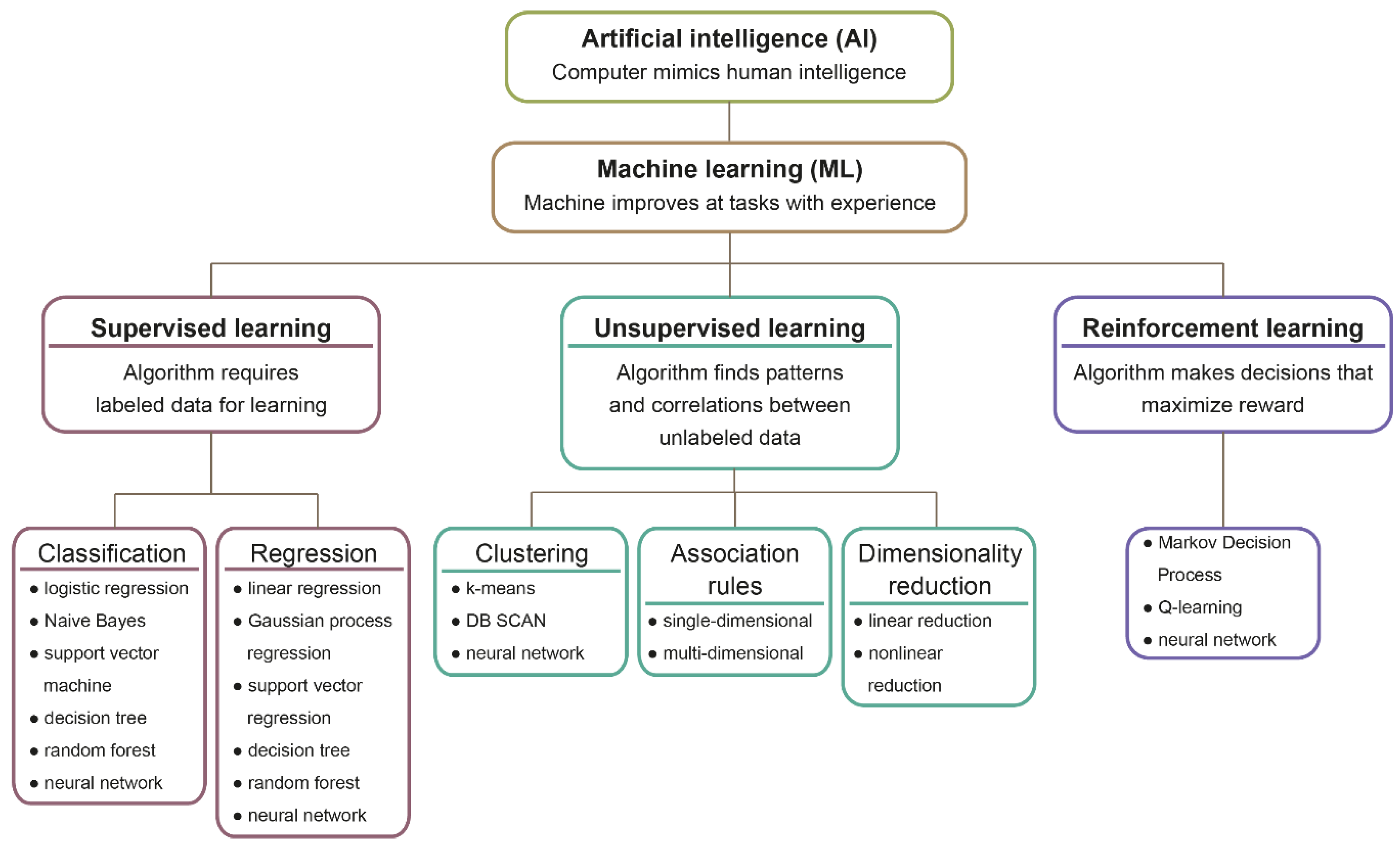
2.2. Machine Learning Models
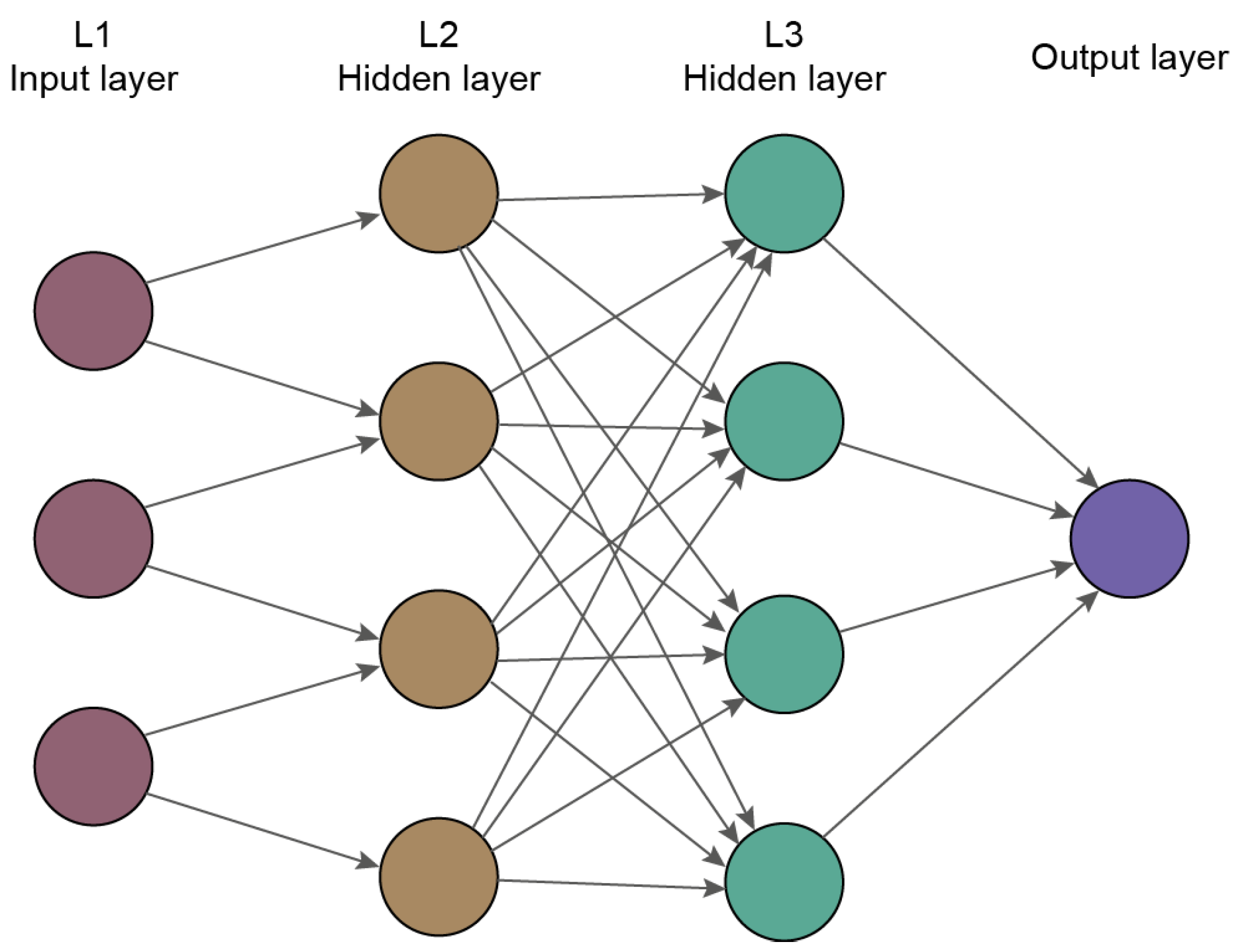
2.3. Deep Learning
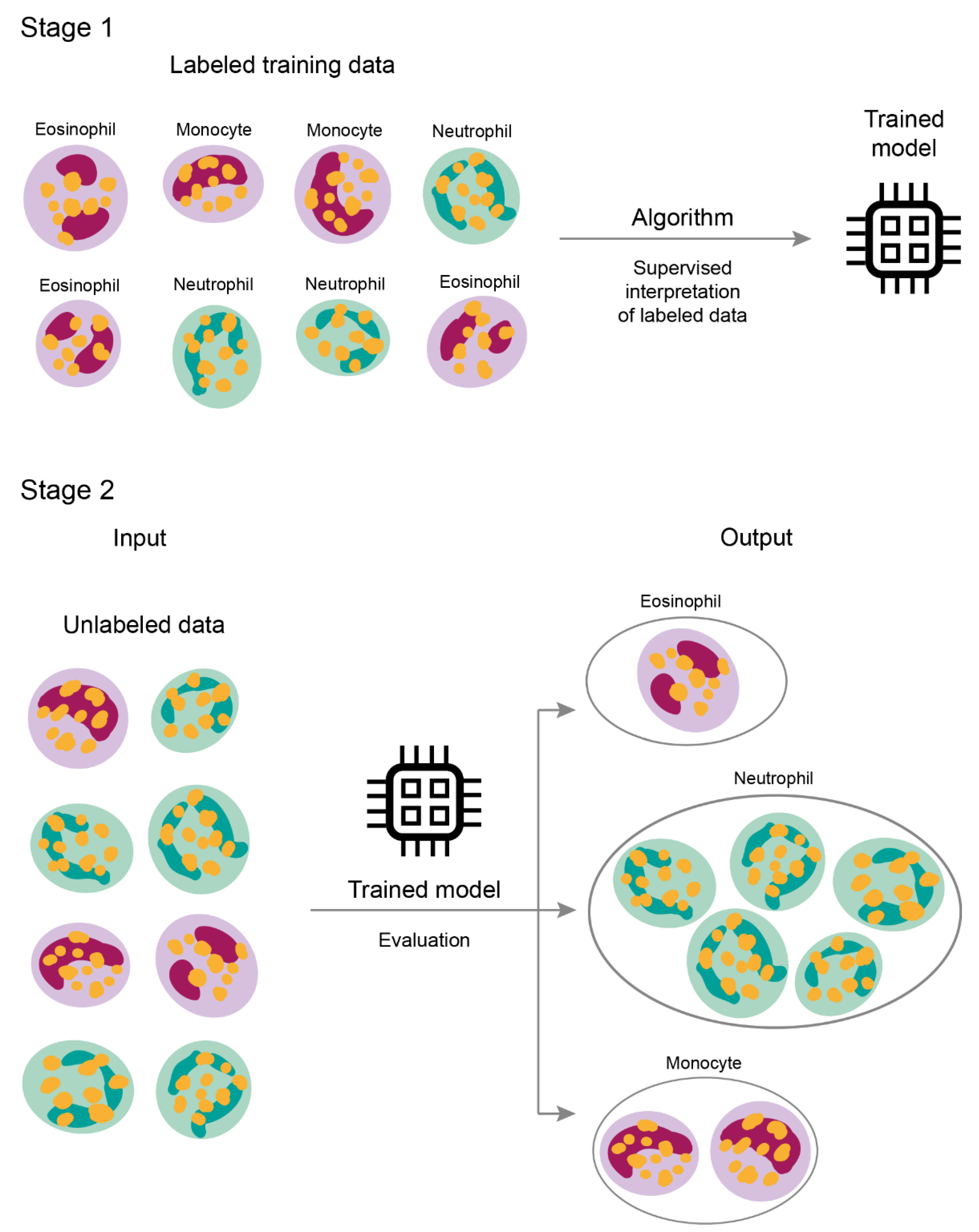
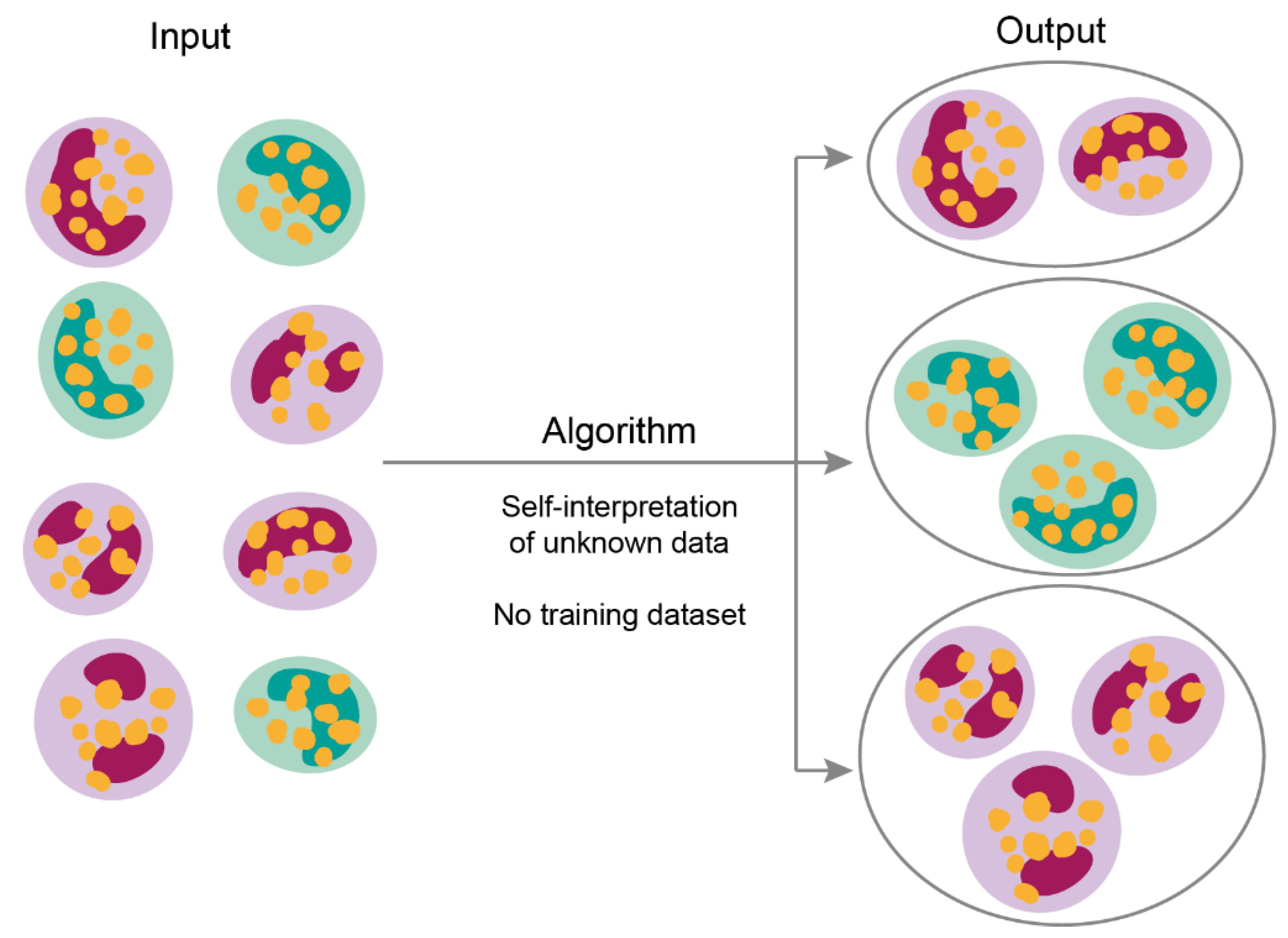
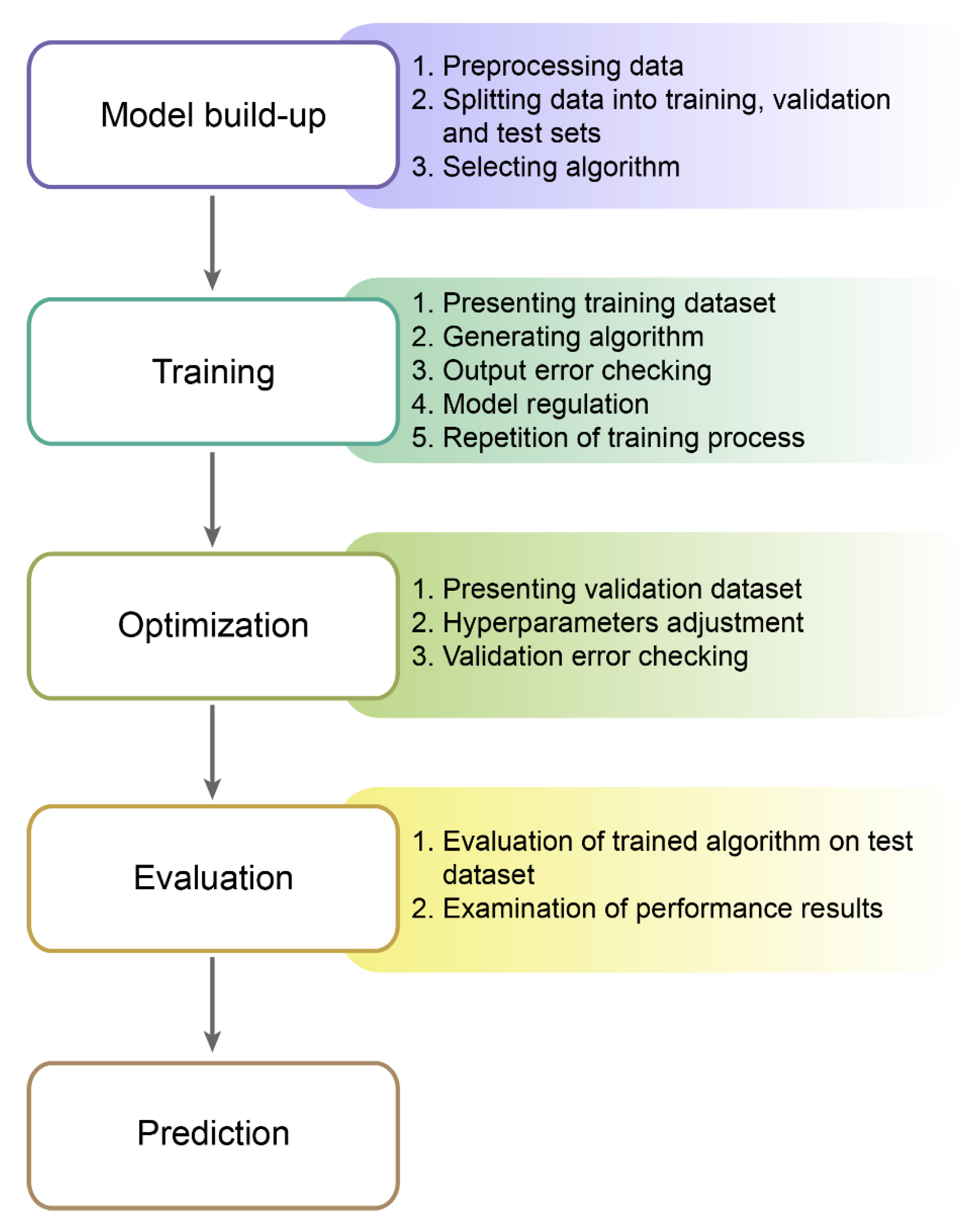
2.4. Machine Learning Process
2.5. Examples of Machine Learning in Everyday Life
3. Application of Machine Learning in Medicine
3.1. Imaging in Medicine
3.2. Personalized Decision Making
3.3. Drug Design
3.4. Infectious Diseases
4. Challenges and Prospects
Author Contributions
Funding
Institutional Review Board Statement
Informed Consent Statement
Data Availability Statement
Acknowledgments
Conflicts of Interest
References
- Ernest, N.; Carroll, D. Genetic Fuzzy based Artificial Intelligence for Unmanned Combat Aerial Vehicle Control in Simulated Air Combat Missions. J. Def. Manag. 2016, 6. [Google Scholar] [CrossRef]
- Morando, M.M.; Tian, Q.; Truong, L.T.; Vu, H.L. Studying the Safety Impact of Autonomous Vehicles Using Simulation-Based Surrogate Safety Measures. J. Adv. Transp. 2018, 2018, 6135183. [Google Scholar] [CrossRef]
- Palmer, C.; Angelelli, L.; Linton, J.; Singh, H.; Muresan, M. Cognitive Cyber Security Assistants–Computationally Deriving Cyber Intelligence and Course of Actions; AAAI: Menlo Park, CA, USA, 2016. [Google Scholar]
- Karakaya, D.; Ulucan, O.; Turkan, M. Electronic Nose and Its Applications: A Survey. Int. J. Autom. Comput. 2020, 17, 179–209. [Google Scholar] [CrossRef] [Green Version]
- Stulp, F.; Sigaud, O. Many regression algorithms, one unified model: A review. Neural Netw. 2015, 69, 60–79. [Google Scholar] [CrossRef] [Green Version]
- Rajkomar, A.; Dean, J.; Kohane, I. Machine learning in medicine. N. Engl. J. Med. 2019, 380, 1347–1358. [Google Scholar] [CrossRef]
- Chandrasekaran, V.; Jordan, M.I. Computational and statistical tradeoffs via convex relaxation. Proc. Natl. Acad. Sci. USA 2013, 110, E1181–E1190. [Google Scholar] [CrossRef] [Green Version]
- Gahlot, S.; Yin, J. Data Optimization for Large Batch Distributed Training of Deep Neural Networks Mallikarjun (Arjun) Shankar. arXiv 2020, arXiv:2012.09272. [Google Scholar]
- Yampolskiy, R.V. Turing test as a defining feature of AI-completeness. Stud. Comput. Intell. 2013, 427, 3–17. [Google Scholar] [CrossRef] [Green Version]
- Aron, J. How innovative is Apple’s new voice assistant, Siri? New Sci. 2011, 212, 24. [Google Scholar] [CrossRef]
- Soltan, S.; Mittal, P.; Vincent, H.; Poor, H.V. BlackIoT: IoT Botnet of High Wattage Devices Can Disrupt the Power Grid BlackIoT: IoT Botnet of High Wattage Devices Can Disrupt the Power Grid. In Proceedings of the 27th USENIX Security Symposium is sponsored by USENIX, Baltimore, MD, USA, 15–17 August 2018; pp. 33–47. [Google Scholar]
- Gudwin, R.R. Evaluating intelligence: A Computational Semiotics perspective. In Proceedings of the IEEE International Conference on Systems, Man and Cybernetics, Nashville, TN, USA, 8–11 October 2000; Volume 3, pp. 2080–2085. [Google Scholar]
- Ghahramani, Z. Probabilistic Machine Learning and Artificial Intelligence. Nature 2015, 521, 452–459. [Google Scholar] [CrossRef]
- Cramer, J.S. The Origins of Logistic Regression. SSRN Electron. J. 2003, 119, 167–178. [Google Scholar] [CrossRef] [Green Version]
- Neelamegam, S.; Ramaraj, E. Karaikudi Classification algorithm in Data mining: An Overview. Int. J. P2P Netw. Trends Technol. 2013, 3, 369–374. [Google Scholar]
- Cortes, C.; Vapnik, V. Support-Vector Networks. Mach. Learn. 1995, 20, 273–297. [Google Scholar] [CrossRef]
- Zou, K.H.; Tuncali, K.; Silverman, S.G. Correlation and simple linear regression. Radiology 2003, 227, 617–622. [Google Scholar] [CrossRef]
- Multiple Linear Regression. In The Concise Encyclopedia of Statistics; Springer: New York, NY, USA, 2008; pp. 364–368.
- Polynomial Regression. In Applied Regression Analysis; Springer: Berlin/Heidelberg, Germany, 2006; pp. 235–268.
- Ho, T.K. Random decision forests. In Proceedings of the International Conference on Document Analysis and Recognition, ICDAR, IEEE Computer Society, Montreal, QC, Canada, 4–16 August 1995; Volume 1, pp. 278–282. [Google Scholar]
- Schubert, E.; Sander, J.; Ester, M.; Kriegel, H.P.; Xu, X. DBSCAN revisited, revisited: Why and how you should (still) use DBSCAN. ACM Trans. Database Syst. 2017, 42, 1–21. [Google Scholar] [CrossRef]
- Libbrecht, M.W.; Noble, W.S. Machine learning applications in genetics and genomics. Nat. Rev. Genet. 2015, 16, 321–332. [Google Scholar] [CrossRef] [Green Version]
- Lloyd, S.; Mohseni, M.; Rebentrost, P. Quantum algorithms for supervised and unsupervised machine learning. arXiv 2013, arXiv:1307.0411. [Google Scholar]
- Wang, M.; Sha, F.; Jordan, M.I. Unsupervised Kernel Dimension Reduction. Adv. Neural Inf. Process. Syst. 2010, 2, 2379–2387. [Google Scholar]
- Caron, M.; Bojanowski, P.; Joulin, A.; Douze, M. Deep Clustering for Unsupervised Learning of Visual Features. In Proceedings of the European Conference on Computer Vision (ECCV), Munich, Germany, 8–14 September 2018; pp. 132–149. [Google Scholar]
- Cios, K.J.; Swiniarski, R.W.; Pedrycz, W.; Kurgan, L.A. Unsupervised Learning: Association Rules. In Data Mining; Springer: New York, NY, USA, 2007; pp. 289–306. [Google Scholar]
- Bifet, A.; Gavaldà, R.; Holmes, G.; Pfahringer, B.; M.I.T. Press Clustering. Machine Learning for Data Streams: With Practical Examples in MOA; MIT Press: Cambridge, MA, USA, 2018; pp. 149–163. ISBN 9780262346047. [Google Scholar]
- Scicluna, B.P.; van Vught, L.A.; Zwinderman, A.H.; Wiewel, M.A.; Davenport, E.E.; Burnham, K.L.; Nürnberg, P.; Schultz, M.J.; Horn, J.; Cremer, O.L.; et al. Classification of patients with sepsis according to blood genomic endotype: A prospective cohort study. Lancet Respir. Med. 2017, 5, 816–826. [Google Scholar] [CrossRef]
- Ayesha, S.; Hanif, M.K.; Talib, R. Overview and comparative study of dimensionality reduction techniques for high dimensional data. Inf. Fusion 2020, 59, 44–58. [Google Scholar] [CrossRef]
- Clark, J.; Provost, F. Unsupervised dimensionality reduction versus supervised regularization for classification from sparse data. Data Min. Knowl. Discov. 2019, 33, 871–916. [Google Scholar] [CrossRef] [Green Version]
- Handl, J.; Knowles, J.; Kell, D.B. Computational cluster validation in post-genomic data analysis. Bioinformatics 2005, 21, 3201–3212. [Google Scholar] [CrossRef] [PubMed] [Green Version]
- Lazar, C.; Taminau, J.; Meganck, S.; Steenhoff, D.; Coletta, A.; Molter, C.; De Schaetzen, V.; Duque, R.; Bersini, H.; Nowé, A. A survey on filter techniques for feature selection in gene expression microarray analysis. IEEE/ACM Trans. Comput. Biol. Bioinforma. 2012, 9, 1106–1119. [Google Scholar] [CrossRef]
- Yang, J.; Wang, H.; Ding, H.; An, N.; Alterovitz, G. Nonlinear dimensionality reduction methods for synthetic biology biobricks’ visualization. BMC Bioinform. 2017, 18, 47. [Google Scholar] [CrossRef] [PubMed] [Green Version]
- Zhu, M.; Xia, J.; Yan, M.; Cai, G.; Yan, J.; Ning, G. Dimensionality Reduction in Complex Medical Data: Improved Self-Adaptive Niche Genetic Algorithm. Comput. Math. Methods Med. 2015, 2015, 794586. [Google Scholar] [CrossRef] [PubMed]
- Peng, C.; Chen, Y.; Kang, Z.; Chen, C.; Cheng, Q. Robust principal component analysis: A factorization-based approach with linear complexity. Inf. Sci. 2020, 513, 581–599. [Google Scholar] [CrossRef]
- Cheplygina, V.; de Bruijne, M.; Pluim, J.P.W. Not-so-supervised: A survey of semi-supervised, multi-instance, and transfer learning in medical image analysis. Med. Image Anal. 2019, 54, 280–296. [Google Scholar] [CrossRef] [Green Version]
- Chi, S.; Li, X.; Tian, Y.; Li, J.; Kong, X.; Ding, K.; Weng, C.; Li, J. Semi-supervised learning to improve generalizability of risk prediction models. J. Biomed. Inform. 2019, 92, 103117. [Google Scholar] [CrossRef]
- Chen, L.; Bentley, P.; Mori, K.; Misawa, K.; Fujiwara, M.; Rueckert, D. Self-supervised learning for medical image analysis using image context restoration. Med. Image Anal. 2019, 58, 101539. [Google Scholar] [CrossRef]
- Doersch, C.; Zisserman, A. Multi-task Self-Supervised Visual Learning. In Proceedings of the IEEE International Conference on Computer Vision, Venice, Italy, 22–29 October 2017; pp. 2051–2060. [Google Scholar]
- Choy, G.; Khalilzadeh, O.; Michalski, M.; Do, S.; Samir, A.E.; Pianykh, O.S.; Geis, J.R.; Pandharipande, P.V.; Brink, J.A.; Dreyer, K.J. Current applications and future impact of machine learning in radiology. Radiology 2018, 288, 318–328. [Google Scholar] [CrossRef]
- François-Lavet, V.; Henderson, P.; Islam, R.; Bellemare, M.G.; Pineau, J. An introduction to deep reinforcement learning. Found. Trends Mach. Learn. 2018, 11, 219–354. [Google Scholar] [CrossRef] [Green Version]
- Silver, D.; Hubert, T.; Schrittwieser, J.; Antonoglou, I.; Lai, M.; Guez, A.; Lanctot, M.; Sifre, L.; Kumaran, D.; Graepel, T.; et al. A general reinforcement learning algorithm that masters chess, shogi, and Go through self-play. Science 2018, 362, 1140–1144. [Google Scholar] [CrossRef] [Green Version]
- Hinton, G.E.; Osindero, S.; Teh, Y.W. A fast learning algorithm for deep belief nets. Neural Comput. 2006, 18, 1527–1554. [Google Scholar] [CrossRef] [PubMed]
- Lecun, Y.; Bengio, Y.; Hinton, G. Deep learning. Nature 2015, 521, 436–444. [Google Scholar] [CrossRef]
- Alom, M.Z.; Taha, T.M.; Yakopcic, C.; Westberg, S.; Sidike, P.; Nasrin, M.S.; Hasan, M.; Van Essen, B.C.; Awwal, A.A.S.; Asari, V.K. A State-of-the-Art Survey on Deep Learning Theory and Architectures. Electronics 2019, 8, 292. [Google Scholar] [CrossRef] [Green Version]
- Marblestone, A.H.; Wayne, G.; Kording, K.P. Toward an integration of deep learning and neuroscience. Front. Comput. Neurosci. 2016, 10, 94. [Google Scholar] [CrossRef] [PubMed]
- Abiodun, O.I.; Jantan, A.; Omolara, A.E.; Dada, K.V.; Mohamed, N.A.E.; Arshad, H. State-of-the-art in artificial neural network applications: A survey. Heliyon 2018, 4, e00938. [Google Scholar] [CrossRef] [PubMed] [Green Version]
- Bevilacqua, V.; Brunetti, A.; Cascarano, G.D.; Guerriero, A.; Pesce, F.; Moschetta, M.; Gesualdo, L. A comparison between two semantic deep learning frameworks for the autosomal dominant polycystic kidney disease segmentation based on magnetic resonance images. BMC Med. Inform. Decis. Mak. 2019, 19, 1–12. [Google Scholar] [CrossRef]
- Altini, N.; Cascarano, G.D.; Brunetti, A.; Marino, F.; Rocchetti, M.T.; Matino, S.; Venere, U.; Rossini, M.; Pesce, F.; Gesualdo, L.; et al. Semantic Segmentation Framework for Glomeruli Detection and Classification in Kidney Histological Sections. Electronics 2020, 9, 503. [Google Scholar] [CrossRef] [Green Version]
- Schmauch, B.; Romagnoni, A.; Pronier, E.; Saillard, C.; Maillé, P.; Calderaro, J.; Kamoun, A.; Sefta, M.; Toldo, S.; Zaslavskiy, M.; et al. A deep learning model to predict RNA-Seq expression of tumours from whole slide images. Nat. Commun. 2020, 11, 1–15. [Google Scholar] [CrossRef]
- Saillard, C.; Schmauch, B.; Laifa, O.; Moarii, M.; Toldo, S.; Zaslavskiy, M.; Pronier, E.; Laurent, A.; Amaddeo, G.; Regnault, H.; et al. Predicting survival after hepatocellular carcinoma resection using deep-learning on histological slides. Hepatology 2020, 72, 2000–2013. [Google Scholar] [CrossRef] [PubMed]
- Long, J.; Shelhamer, E.; Darrell, T. Fully Convolutional Networks for Semantic Segmentation. IEEE Trans. Pattern Anal. Mach. Intell. 2014, 39, 640–651. [Google Scholar]
- Ronneberger, O.; Fischer, P.; Brox, T. U-net: Convolutional networks for biomedical image segmentation. In Lecture Notes in Computer Science (Including Subseries Lecture Notes in Artificial Intelligence and Lecture Notes in Bioinformatics); Springer: Berlin/Heidelberg, Germany, 2015; Volume 9351, pp. 234–241. [Google Scholar]
- Milletari, F.; Navab, N.; Ahmadi, S.-A. V-Net: Fully Convolutional Neural Networks for Volumetric Medical Image Segmentation. In Proceedings of the 2016 Fourth International Conference on 3D Vision (3DV), Stanford, CA, USA, 25–28 October 2016; pp. 565–571. [Google Scholar]
- Pinheiro, G.R.; Voltoline, R.; Bento, M.; Rittner, L. V-net and u-net for ischemic stroke lesion segmentation in a small dataset of perfusion data. In Lecture Notes in Computer Science (Including Subseries Lecture Notes in Artificial Intelligence and Lecture Notes in Bioinformatics); Springer: Berlin/Heidelberg, Germany, 2019; Volume 11383 LNCS, pp. 301–309. [Google Scholar]
- Nugaliyadde, A.; Wong, K.W.; Parry, J.; Sohel, F.; Laga, H.; Somaratne, U.V.; Yeomans, C.; Foster, O. RCNN for Region of Interest Detection in Whole Slide Images; Springer: Cham, Switzerland, 2020; pp. 625–632. ISBN 9783030638221. [Google Scholar]
- Brunetti, A.; Carnimeo, L.; Trotta, G.F.; Bevilacqua, V. Computer-assisted frameworks for classification of liver, breast and blood neoplasias via neural networks: A survey based on medical images. Neurocomputing 2019, 335, 274–298. [Google Scholar] [CrossRef]
- Girshick, R. Fast R-CNN; IEEE: New York, NY, USA, 2015; ISBN 978-1-4673-8391-2. [Google Scholar]
- Ren, S.; He, K.; Girshick, R.; Sun, J. Faster R-CNN: Towards Real-Time Object Detection with Region Proposal Networks. IEEE Trans. Pattern Anal. Mach. Intell. 2017, 39, 1137–1149. [Google Scholar] [CrossRef] [PubMed] [Green Version]
- He, K.; Gkioxari, G.; Dollár, P.; Girshick, R. Mask R-CNN. IEEE Trans. Pattern Anal. Mach. Intell. 2020, 42, 386–397. [Google Scholar] [CrossRef]
- Kriegeskorte, N.; Golan, T. Neural network models and deep learning. Curr. Biol. 2019, 29, R231–R236. [Google Scholar] [CrossRef] [PubMed]
- Lyu, C.; Chen, B.; Ren, Y.; Ji, D. Long short-term memory RNN for biomedical named entity recognition. BMC Bioinform. 2017, 18, 462. [Google Scholar] [CrossRef] [PubMed]
- Navamani, T.M. Efficient Deep Learning Approaches for Health Informatics. In Deep Learning and Parallel Computing Environment for Bioengineering Systems; Elsevier: Amsterdam, The Netherlands, 2019; pp. 123–137. [Google Scholar]
- Zhang, S.; Zhang, C.; Yang, Q. Data preparation for data mining. Appl. Artif. Intell. 2003, 17, 375–381. [Google Scholar] [CrossRef]
- Chicco, D. Ten quick tips for machine learning in computational biology. Chicco BioData Min. 2017, 10, 35. [Google Scholar] [CrossRef]
- Powell, M.; Hosseini, M.; Collins, J.; Callahan-Flintoft, C.; Jones, W.; Bowman, H.; Wyble, B. I Tried a Bunch of Things: The Dangers of Unexpected Overfitting in Classification. bioRxiv 2016, 119, 456–467. [Google Scholar] [CrossRef]
- Boulesteix, A.-L. Ten Simple Rules for Reducing Overoptimistic Reporting in Methodological Computational Research. PLoS Comput. Biol. 2015, 11, e1004191. [Google Scholar] [CrossRef] [Green Version]
- Grégoire, G. Simple linear regression. In EAS Publications Series; EDP Sciences: Les Ulis, France, 2015; Volume 66, pp. 19–39. [Google Scholar]
- Tarca, A.L.; Carey, V.J.; Chen, X.; Romero, R.; Drăghici, S. Machine Learning and Its Applications to Biology. PLoS Comput. Biol. 2007, 3, e116. [Google Scholar] [CrossRef] [PubMed]
- Models for Machine Learning; IBM Developer: Armonk, NY, USA, 2017.
- Mehta, P.; Bukov, M.; Wang, C.H.; Day, A.G.R.; Richardson, C.; Fisher, C.K.; Schwab, D.J. Physics Reports; Elsevier B.V.: Amsterdam, The Netherlands, 2019; pp. 1–124. [Google Scholar]
- Online Payment Fraud. Available online: https://www.ravelin.com/insights/online-payment-fraud#thethreepillarsoffraudprotection (accessed on 19 November 2020).
- Baker, J. Using Machine Learning to Detect Financial Fraud. Bus. Stud. Sch. Creat. Work 2019, 6. Available online: https://jayscholar.etown.edu/busstu/6 (accessed on 19 November 2020).
- Wei, J.; He, J.; Chen, K.; Zhou, Y.; Tang, Z. Collaborative Filtering and Deep Learning Based Hybrid Recommendation for Cold Start Problem; IEEE: New York, NY, USA, 2016. [Google Scholar] [CrossRef] [Green Version]
- Technology—Waymo. Available online: https://waymo.com/tech/ (accessed on 19 November 2020).
- Brynjolfsson, E.; Rock, D.; Syverson, C.; Abrams, E.; Agrawal, A.; Autor, D.; Benzell, S.; Gans, J.; Goldfarb, A.; Goolsbee, A.; et al. Nber Working Paper Series Artificial Intelligence and the Modern Productivity Paradox: A Clash of Expectations and Statistics; National Bureau of Economic Research: Cambridge, MA, USA, 2017. [Google Scholar]
- Chu, K.C.; Feldmann, R.J.; Shapiro, B.; Hazard, G.F.; Geran, R.I. Pattern Recognition and Structure-Activity Relation Studies. Computer-Assisted Prediction of Antitumor Activity in Structurally Diverse Drugs in an Experimental Mouse Brain Tumor System. J. Med. Chem. 1975, 18, 539–545. [Google Scholar] [CrossRef] [PubMed]
- Shortliffe, E.H. Computer-Based Medical Consultations: MYCIN; Elsevier: New York, NY, USA, 1976; ISBN 978-0444569691. [Google Scholar]
- Finlayson, S.G.; Bowers, J.D.; Ito, J.; Zittrain, J.L.; Beam, A.L.; Kohane, I.S. Adversarial attacks on medical machine learning. Science 2019, 363, 1287–1289. [Google Scholar] [CrossRef] [PubMed]
- FDA’s Comprehensive Effort to Advance New Innovations: Initiatives to Modernize for Innovation | FDA. Available online: https://www.fda.gov/news-events/fda-voices/fdas-comprehensive-effort-advance-new-innovations-initiatives-modernize-innovation (accessed on 6 January 2021).
- Zhu, B.; Liu, J.Z.; Cauley, S.F.; Rosen, B.R.; Rosen, M.S. Image reconstruction by domain-transform manifold learning. Nature 2018, 555, 487–492. [Google Scholar] [CrossRef] [PubMed] [Green Version]
- Kermany, D.S.; Goldbaum, M.; Cai, W.; Valentim, C.C.S.; Liang, H.; Baxter, S.L.; McKeown, A.; Yang, G.; Wu, X.; Yan, F.; et al. Identifying Medical Diagnoses and Treatable Diseases by Image-Based Deep Learning. Cell 2018, 172, 1122–1131.e9. [Google Scholar] [CrossRef] [PubMed]
- Christiansen, E.M.; Yang, S.J.; Ando, D.M.; Javaherian, A.; Skibinski, G.; Lipnick, S.; Mount, E.; O’Neil, A.; Shah, K.; Lee, A.K.; et al. In Silico Labeling: Predicting Fluorescent Labels in Unlabeled Images. Cell 2018, 173, 792–803.e19. [Google Scholar] [CrossRef] [PubMed] [Green Version]
- Tomašev, N.; Glorot, X.; Rae, J.W.; Zielinski, M.; Askham, H.; Saraiva, A.; Mottram, A.; Meyer, C.; Ravuri, S.; Protsyuk, I.; et al. A clinically applicable approach to continuous prediction of future acute kidney injury. Nature 2019, 572, 116–119. [Google Scholar] [CrossRef]
- Li, J.; Pan, C.; Zhang, S.; Spin, J.M.; Deng, A.; Leung, L.L.K.; Dalman, R.L.; Tsao, P.S.; Snyder, M. Decoding the Genomics of Abdominal Aortic Aneurysm. Cell 2018, 174, 1361–1372. [Google Scholar] [CrossRef] [Green Version]
- Jamthikar, A.; Gupta, D.; Khanna, N.N.; Saba, L.; Araki, T.; Viskovic, K.; Suri, H.S.; Gupta, A.; Mavrogeni, S.; Turk, M.; et al. A low-cost machine learning-based cardiovascular/stroke risk assessment system: Integration of conventional factors with image phenotypes. Cardiovasc. Diagn. Ther. 2019, 9, 420–430. [Google Scholar] [CrossRef] [Green Version]
- Adler, E.D.; Voors, A.A.; Klein, L.; Macheret, F.; Braun, O.O.; Urey, M.A.; Zhu, W.; Sama, I.; Tadel, M.; Campagnari, C.; et al. Improving risk prediction in heart failure using machine learning. Eur. J. Heart Fail. 2019, 22, 139–147. [Google Scholar] [CrossRef] [PubMed]
- Zeevi, D.; Korem, T.; Zmora, N.; Israeli, D.; Rothschild, D.; Weinberger, A.; Ben-Yacov, O.; Lador, D.; Avnit-Sagi, T.; Lotan-Pompan, M.; et al. Personalized Nutrition by Prediction of Glycemic Responses. Cell 2015, 163, 1079–1094. [Google Scholar] [CrossRef] [PubMed] [Green Version]
- Yang, J.H.; Wright, S.N.; Hamblin, M.; McCloskey, D.; Alcantar, M.A.; Schrübbers, L.; Lopatkin, A.J.; Satish, S.; Nili, A.; Palsson, B.O.; et al. A White-Box Machine Learning Approach for Revealing Antibiotic Mechanisms of Action. Cell 2019, 177, 1649–1661.e9. [Google Scholar] [CrossRef] [PubMed]
- Granda, J.M.; Donina, L.; Dragone, V.; Long, D.L.; Cronin, L. Controlling an organic synthesis robot with machine learning to search for new reactivity. Nature 2018, 559, 377–381. [Google Scholar] [CrossRef]
- Jayaraj, P.B.; Jain, S. Ligand based virtual screening using SVM on GPU. Comput. Biol. Chem. 2019, 83, 107143. [Google Scholar] [CrossRef]
- Stokes, J.M.; Yang, K.; Swanson, K.; Jin, W.; Cubillos-Ruiz, A.; Donghia, N.M.; MacNair, C.R.; French, S.; Carfrae, L.A.; Bloom-Ackerman, Z.; et al. A Deep Learning Approach to Antibiotic Discovery. Cell 2020, 180, 688–702.e13. [Google Scholar] [CrossRef] [Green Version]
- Popova, M.; Isayev, O.; Tropsha, A. Deep reinforcement learning for de novo drug design. Sci. Adv. 2018, 4, eaap7885. [Google Scholar] [CrossRef] [Green Version]
- Lei, D.; Pinaya, W.H.L.; Young, J.; van Amelsvoort, T.; Marcelis, M.; Donohoe, G.; Mothersill, D.O.; Corvin, A.; Vieira, S.; Huang, X.; et al. Integrating machining learning and multimodal neuroimaging to detect schizophrenia at the level of the individual. Hum. Brain Mapp. 2019, 41, 1119–1135. [Google Scholar] [CrossRef] [Green Version]
- Mellema, C.; Treacher, A.; Nguyen, K.; Montillo, A. Multiple Deep Learning Architectures Achieve Superior Performance Diagnosing Autism Spectrum Disorder Using Features Previously Extracted from Structural and Functional MRI. Proc. IEEE Int. Symp. Biomed. Imaging 2019, 2019, 1891–1895. [Google Scholar] [CrossRef]
- Law, M.T.; Traboulsee, A.L.; Li, D.K.; Carruthers, R.L.; Freedman, M.S.; Kolind, S.H.; Tam, R. Machine learning in secondary progressive multiple sclerosis: An improved predictive model for short-term disability progression. Mult. Scler. J. Exp. Transl. Clin. 2019, 5, 2055217319885983. [Google Scholar] [CrossRef] [PubMed]
- Cascarano, G.D.; Loconsole, C.; Brunetti, A.; Lattarulo, A.; Buongiorno, D.; Losavio, G.; Di Sciascio, E.; Bevilacqua, V. Biometric handwriting analysis to support Parkinson’s Disease assessment and grading. BMC Med. Inform. Decis. Mak. 2019, 19, 252. [Google Scholar] [CrossRef] [PubMed] [Green Version]
- Trotta, G.F.; Pellicciari, R.; Boccaccio, A.; Brunetti, A.; Cascarano, G.D.; Manghisi, V.M.; Fiorentino, M.; Uva, A.E.; Defazio, G.; Bevilacqua, V. A neural network-based software to recognise blepharospasm symptoms and to measure eye closure time. Comput. Biol. Med. 2019, 112, 103376. [Google Scholar] [CrossRef] [PubMed]
- Kök, H.; Acilar, A.M.; İzgi, M.S. Usage and comparison of artificial intelligence algorithms for determination of growth and development by cervical vertebrae stages in orthodontics. Prog. Orthod. 2019, 20, 41. [Google Scholar] [CrossRef] [PubMed]
- Kim, J.; Chang, H.L.; Kim, D.; Jang, D.H.; Park, I.; Kim, K. Machine learning for prediction of septic shock at initial triage in emergency department. J. Crit. Care 2020, 55, 163–170. [Google Scholar] [CrossRef] [PubMed]
- Stehrer, R.; Hingsammer, L.; Staudigl, C.; Hunger, S.; Malek, M.; Jacob, M.; Meier, J. Machine learning based prediction of perioperative blood loss in orthognathic surgery. J. Craniomaxillofac. Surg. 2019, 47, 1676–1681. [Google Scholar] [CrossRef]
- Liu, Z.; Huang, S.; Lu, W.; Su, Z.; Yin, X.; Liang, H.; Zhang, H. Modeling the trend of coronavirus disease 2019 and restoration of operational capability of metropolitan medical service in China: A machine learning and mathematical model-based analysis. Glob. Heal. Res. Policy 2020, 5, 1–11. [Google Scholar] [CrossRef]
- Randhawa, G.S.; Soltysiak, M.P.M.; El Roz, H.; de Souza, C.P.E.; Hill, K.A.; Kari, L. Machine learning using intrinsic genomic signatures for rapid classification of novel pathogens: COVID-19 case study. PLoS ONE 2020, 15, e0232391. [Google Scholar] [CrossRef] [Green Version]
- Mei, X.; Lee, H.-C.; Diao, K.-Y.; Huang, M.; Lin, B.; Liu, C.; Xie, Z.; Ma, Y.; Robson, P.M.; Chung, M.; et al. Artificial intelligence-enabled rapid diagnosis of patients with COVID-19. Nat. Med. 2020, 26, 1224–1228. [Google Scholar] [CrossRef]
- Hornbrook, M.C.; Goshen, R.; Choman, E.; O’Keeffe-Rosetti, M.; Kinar, Y.; Liles, E.G.; Rust, K.C. Early Colorectal Cancer Detected by Machine Learning Model Using Gender, Age, and Complete Blood Count Data. Dig. Dis. Sci. 2017, 62, 2719–2727. [Google Scholar] [CrossRef] [Green Version]
- Kinar, Y.; Kalkstein, N.; Akiva, P.; Levin, B.; Half, E.E.; Goldshtein, I.; Chodick, G. Development and validation of a predictive model for detection of colorectal cancer in primary care by analysis of complete blood counts: A binational retrospective study. J. Am. Med. Inform. Assoc. 2016, 972, 879–890. [Google Scholar] [CrossRef] [PubMed] [Green Version]
- Ellrott, K.; Bailey, M.H.; Saksena, G.; Covington, K.R.; Kandoth, C.; Stewart, C.; Hess, J.; Ma, S.; Chiotti, K.E.; McLellan, M.; et al. Scalable Open Science Approach for Mutation Calling of Tumor Exomes Using Multiple Genomic Pipelines. Cell Syst. 2018, 6, 271–281.e7. [Google Scholar] [CrossRef] [PubMed] [Green Version]
- Bailey, M.H.; Tokheim, C.; Porta-Pardo, E.; Sengupta, S.; Bertrand, D.; Weerasinghe, A.; Colaprico, A.; Wendl, M.C.; Kim, J.; Reardon, B.; et al. Comprehensive Characterization of Cancer Driver Genes and Mutations. Cell 2018, 173, 371–385.e18. [Google Scholar] [CrossRef] [PubMed] [Green Version]
- Lu, C.F.; Hsu, F.T.; Hsieh, K.L.C.; Kao, Y.C.J.; Cheng, S.J.; Hsu, J.B.K.; Tsai, P.H.; Chen, R.J.; Huang, C.C.; Yen, Y.; et al. Machine learning–based radiomics for molecular subtyping of gliomas. Clin. Cancer Res. 2018, 24, 4429–4436. [Google Scholar] [CrossRef] [PubMed] [Green Version]
- Kather, J.N.; Weis, C.A.; Bianconi, F.; Melchers, S.M.; Schad, L.R.; Gaiser, T.; Marx, A.; Zöllner, F.G. Multi-class texture analysis in colorectal cancer histology. Sci. Rep. 2016, 6, 27988. [Google Scholar] [CrossRef] [PubMed]
- Cammarota, G.; Ianiro, G.; Ahern, A.; Carbone, C.; Temko, A.; Claesson, M.J.; Gasbarrini, A.; Tortora, G. Gut microbiome, big data and machine learning to promote precision medicine for cancer. Nat. Rev. Gastroenterol. Hepatol. 2020, 17, 635–648. [Google Scholar] [CrossRef] [PubMed]
- Louise Pouncey, A.; James Scott, A.; Leslie Alexander, J.; Marchesi, J.; Kinross, J. Gut microbiota, chemotherapy and the host: The influence of the gut microbiota on cancer treatment. Ecancermedicalscience 2018, 12, 868. [Google Scholar] [CrossRef] [Green Version]
- Song, J.; Wang, L.; Ng, N.N.; Zhao, M.; Shi, J.; Wu, N.; Li, W.; Liu, Z.; Yeom, K.W.; Tian, J. Development and Validation of a Machine Learning Model to Explore Tyrosine Kinase Inhibitor Response in Patients With Stage IV EGFR Variant–Positive Non–Small Cell Lung Cancer. JAMA Netw. Open 2020, 3, e2030442. [Google Scholar] [CrossRef]
- Linder, N.; Konsti, J.; Turkki, R.; Rahtu, E.; Lundin, M.; Nordling, S.; Haglund, C.; Ahonen, T.; Pietikäinen, M.; Lundin, J. Identification of tumor epithelium and stroma in tissue microarrays using texture analysis. Diagn. Pathol. 2012, 7, 22. [Google Scholar] [CrossRef] [Green Version]
- Garcia-Canadilla, P.; Sanchez-Martinez, S.; Crispi, F.; Bijnens, B. Machine Learning in Fetal Cardiology: What to Expect. Fetal Diagn. Ther. 2020, 47, 363–372. [Google Scholar] [CrossRef]
- Vashist, S.; Schneider, E.; Luong, J. Commercial Smartphone-Based Devices and Smart Applications for Personalized Healthcare Monitoring and Management. Diagnostics 2014, 4, 104–128. [Google Scholar] [CrossRef] [PubMed]
- Nedungadi, P.; Jayakumar, A.; Raman, R. Personalized Health Monitoring System for Managing Well-Being in Rural Areas. J. Med. Syst. 2018, 42, 22. [Google Scholar] [CrossRef] [PubMed]
- Barrios, M.; Jimeno, M.; Villalba, P.; Navarro, E. Novel Data Mining Methodology for Healthcare Applied to a New Model to Diagnose Metabolic Syndrome without a Blood Test. Diagnostics 2019, 9, 192. [Google Scholar] [CrossRef] [PubMed] [Green Version]
- Heaven, D. Why deep-learning AIs are so easy to fool. Nature 2019, 574, 163–166. [Google Scholar] [CrossRef]
- Char, D.S.; Shah, N.H.; Magnus, D. Implementing machine learning in health care ’ addressing ethical challenges. N. Engl. J. Med. 2018, 378, 981–983. [Google Scholar] [CrossRef] [Green Version]
- Shank, D.B.; Graves, C.; Gott, A.; Gamez, P.; Rodriguez, S. Feeling our way to machine minds: People’s emotions when perceiving mind in artificial intelligence. Comput. Hum. Behav. 2019, 98, 256–266. [Google Scholar] [CrossRef]


| Element of ML | Description |
|---|---|
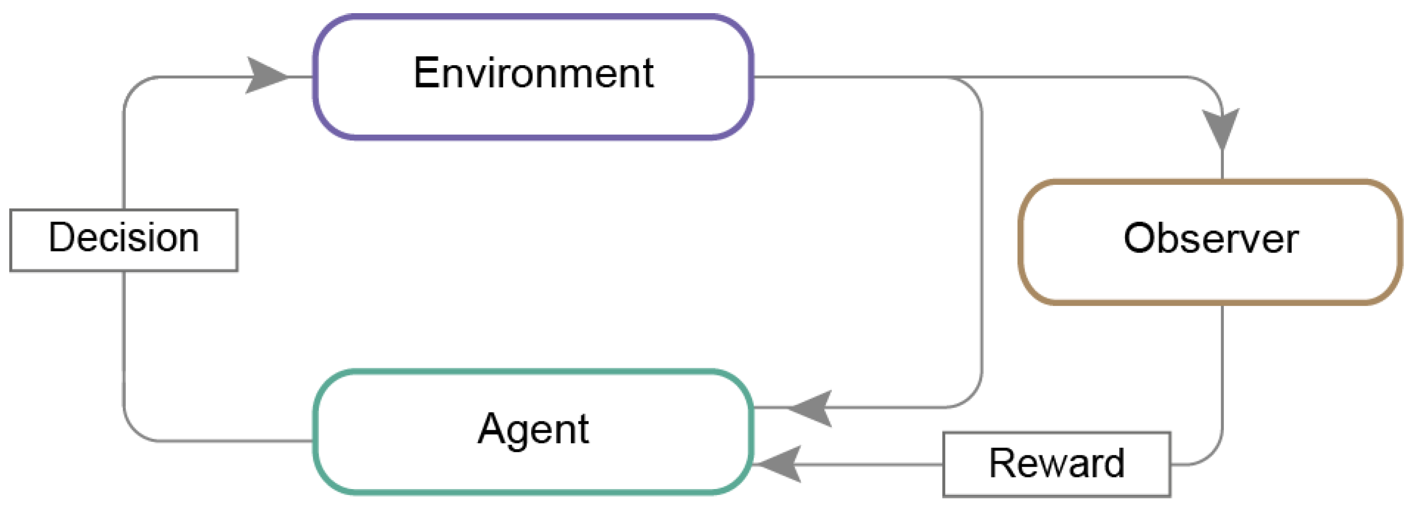
| Artificial agent | An independent program that acts regarding received signals from its environment to meet designated goals. Such an agent is autonomous because it can perform without human or any other system. |
| Clustering | Grouping data points with similar features which differ from other data points containing exceedingly different properties. |
| Environment | A task or a problem that needs to be resolved by the agent. The environment interacts with the agent by executing each received action, sending its current state and reward, linked with agents’ undertaken actions. |
| Feature | An individual quantifiable attribute for the presented event, as the input color or size. |
| Hyperparameters | Parameters that cannot be estimated from training data and are optimized beyond the model. They can be tuned manually in order to get the best possible results. |
| Input | A piece of information or data provided to the machine in pictures, numbers, text, sounds, or other types. |
| Label | A description of the input or output; for example, an x-ray of lungs may have the label “lung”. |
| Layer | The most prominent structure in deep learning. Each layer consists of nodes called neurons, connected, creating together a neural network. The connections between neurons are weighted, and in consequence, the processing signal is increased or decreased. |
| Output | Predicted data generated by a machine learning model with an association with the further given input. |
| Reward | Information from the environment (or supervisor) to an agent about the action’s precision. The reward can be positive or negative, depending on if the action was correct or not. It allows concluding behavior in a particular state. |
| Algorithm | Prediction | References |
|---|---|---|
| Algorithms Applied in Supervised Learning | ||
| Probabilistic model (classification) | Probability distributions are applied to represent all uncertain, unnoticed quantities (including structural, parametric, and noise-related aspects) and their relation to current data. | [13] |
| Logistic regression (classification) | Predicts probability comparing to a logit function or decision trees, where the algorithm divides data according to the essential assets making these groups extremely distinct. | [14] |
| Naïve Bayes classifier (classification) | Assumes that a feature presence in a class is unrelated to any other element’s presence. | [15] |
| Support vector machine (classification) | The algorithm finds the hyperplane with the immense distance of points from both classes. | [16] |
| Simple linear regression (value prediction) | Estimates the relationship of one independent to one dependent variable using a straight line. | [17] |
| Multiple linear regression (value prediction) | Estimates the relationship of at least two independents to one dependent variable using a hyperplane. | [18] |
| Polynomial regression (value prediction) | Kind of linear regression in which the relationship between the independent and dependent variables is projected as an n-degree polynomial. | [19] |
| Decision-tree (classification or value prediction) | A non-parametric algorithm constructs classification or regression in the form of a tree structure. It splits a data set into further small subsets while gradually expanding the associated decision tree. | [15] |
| Random forest (classification or value prediction) | Set consisting of a few decision trees, out of which a class dominant (classification) or expected average (regression) of individual trees is determined. | [20] |
| Algorithms Applied in Supervised Learning | ||
| K-means (clustering) | Clusters are formed by the proximity of data points to the middle of cluster—the most minimal distance of data points in the center. | [21] |
| DBSCAN (clustering) | Consists of clustering points within nearby neighbors (high-density region), outlying those being comparatively far away (low-density region). | [21] |
| Algorithms Applied in Reinforcement Learning | ||
| Markov Decision Process | A mathematical approach where sets of states and rewards are finite. The probability of movement into a new state is influenced by the previous one and the selected action. The likelihood of the transition from state “a” to state “b” is defined with a reward from taking particular action. | [21] |
| Q-learning | Discovers an optimum policy and maximizes reward for the whole following steps launched from the present state. Hither, the agent acts randomly, exploring and discovering new states or exploiting provided information on the possibility of initiating action in the current state. | [20] |
| Branch of Medicine | Application | Description | ML Method | References |
|---|---|---|---|---|
| Radiology | Image reconstruction | High resolution and quality images | Deep neural network | [81] |
| Image analysis | Faster and more accurate analysis | Convolutional neural network and transfer learning | [82] | |
| Pathology | in silico labeling | No need for cell/tissue staining; faster and cheaper analysis | Deep neural network | [83] |
| Nephrology | Prediction of organ injury | Detection of kidney injury up to 48 h in advance, which enable early treatment | Deep neural network | [84] |
| Image analysis and diagnosis | Polycystic kidneys segmentation | Convolutional neural network | [48] | |
| Cardiology | Personalized decision making | Early detection of abdominal aortic aneurysm | Agnostic learning | [85] |
| Improvement of ML techniques to cardiovascular disease risk prediction | Principal component analysis and random forest | [86] | ||
| Mortality risk prediction model in patients with a heart attack | Decision tree | [87] | ||
| Nutrition | Personalized decision making | More accurate, personalized postmeal glucose response prediction | Boosted decision tree | [88] |
| Diabetology | ||||
| Transplantology | Computer-Aided Diagnosis | Estimation of global glomerulosclerosis before kidney transplantation | Convolutional Neural Network | [49] |
| Pharmacology | Studying drug mechanisms of action | New mechanisms of antibiotic action | White-box machine learning | [89] |
| Predicting compounds reactivity | Automated tool for reactivity screening | Supported vector machine | [90] | |
| Ligands screening | Faster screening of compounds that bind to the target | Supported vector machine | [91] | |
| Compounds screening | Discovery of new antibacterial molecules | Deep neural network | [92] | |
| De novo drug design | Generation of libraries of a novel, potentially therapeutical compounds with desired properties | Reinforcement neural network | [93] | |
| Psychiatry | Image analysis and diagnosis | MRI image analysis and fast diagnoses of schizophrenia | Supported vector machine | [94] |
| Neurology | Image analysis and diagnosis | MRI image analysis and diagnoses of autism spectrum disorder | A naïve Bayes, supported vector machine, random forest, extremely randomized trees, adaptive boosting, gradient boosting with decision tree base, logistic regression, neural network | [95] |
| Prognosis the course of the disease | Prediction of progression of disability of multiple sclerosis patients | Decision tree, logistic regression, supported vector machine | [96] | |
| Diagnosis support | Mild and moderate Parkinson’s Disease detection and rating | Artificial Neural Network | [97] | |
| Diagnosis support | Blepharospasm detection and rating | Artificial Neural Network | [98] | |
| Dentistry | Personalized decision making | Determination of optimal bone age for orthodontal treatment | k-nearest neighbors, a naïve Bayes, decision tree, neural network, supported vector machine, random forest, logistic regression | [99] |
| Emergency medicine | Personalized decision making | Triage and prediction of septic shock in the emergency department | Supported vector machine, gradient- boosting machine, random forest, multivariate adaptive regression splines, least absolute shrinkage and selection operator, ridge regression | [100] |
| Surgery | Personalized decision making | Prediction of the amount of lost blood during surgery | Random forest | [101] |
| Infectious diseases | Estimation of epidemic trend | Prediction of number of confirmed cases, deaths, and recoveries during coronavirus outbreak | Neural network | [102] |
| The evolutionary history of viruses | Classification of novel pathogens and determination of the origin of the viruses | Supervised learning with digital processing (MLDSP) | [103] | |
| Diagnoses of infectious diseases | Early diagnoses of COVID-19 | Convolutional neural network, support vector machine, random forest, and multilayer perception | [104] | |
| Oncology | Patients screening | Indicating increased risk of colorectal cancer, early cancer detection | Decision tree | [105,106] |
| Cancer research | New cancer driver genes and mutations discovery | Random forest | [107,108] | |
| Cancer subtypes classification | three-level classification model of gliomas | Support vector machine, decision tree | [109] | |
| Image analysis and cancer diagnosis | Prediction of gene expression | Deep learning | [50] | |
| Improvement of image analysis | Tumor microenvironment components classification in colorectal cancer histological images | 1-nearest neighbor, support vector machine, decision tree | [110] | |
| Cancer development preventing | Gut microbiota analysis in search of biomarkers of neoplasms | Convolutional neural network, support vector machine, random forest, and multilayer perception | [111] | |
| Tolerability of cancer therapies | Identification of microbial signatures affecting gastrointestinal drug toxicity | A naïve Bayes, supported vector machine, random forest, extremely randomized trees, adaptive boosting, gradient boosting with decision tree base, logistic regression, neural network | [111,112] | |
| Image analysis and prognosis the course of the disease | Predicting hepatocellular carcinoma patients’ survival after tumor resection based on histological slides | Deep learning | [51] | |
| Treatment response prediction | Prediction of therapy outcomes in EGFR variant-positive non-small cell lung cancer patients | Deep learning | [113] | |
| Image analysis | Tumor microenvironments components identification | Support vector machine | [114] |
Publisher’s Note: MDPI stays neutral with regard to jurisdictional claims in published maps and institutional affiliations. |
© 2021 by the authors. Licensee MDPI, Basel, Switzerland. This article is an open access article distributed under the terms and conditions of the Creative Commons Attribution (CC BY) license (http://creativecommons.org/licenses/by/4.0/).
Share and Cite
Koteluk, O.; Wartecki, A.; Mazurek, S.; Kołodziejczak, I.; Mackiewicz, A. How Do Machines Learn? Artificial Intelligence as a New Era in Medicine. J. Pers. Med. 2021, 11, 32. https://0-doi-org.brum.beds.ac.uk/10.3390/jpm11010032
Koteluk O, Wartecki A, Mazurek S, Kołodziejczak I, Mackiewicz A. How Do Machines Learn? Artificial Intelligence as a New Era in Medicine. Journal of Personalized Medicine. 2021; 11(1):32. https://0-doi-org.brum.beds.ac.uk/10.3390/jpm11010032
Chicago/Turabian StyleKoteluk, Oliwia, Adrian Wartecki, Sylwia Mazurek, Iga Kołodziejczak, and Andrzej Mackiewicz. 2021. "How Do Machines Learn? Artificial Intelligence as a New Era in Medicine" Journal of Personalized Medicine 11, no. 1: 32. https://0-doi-org.brum.beds.ac.uk/10.3390/jpm11010032