Article

The Hunt for Environmental Noise in Virgo during the Third Observing Run

by
Irene Fiori
1,
Federico Paoletti
2,
Maria Concetta Tringali
1,3,*,
Kamiel Janssens
4,
Christos Karathanasis
5,
Alexis Menéndez-Vázquez
5,
Alba Romero-Rodríguez
5,
Ryosuke Sugimoto
6,
Tatsuki Washimi
7,
Valerio Boschi
2,
Antonino Chiummo
1,
Marek Cieślar
8,
Rosario De Rosa
9,10,
Camilla De Rossi
1,
Francesco Di Renzo
2,11,
Ilaria Nardecchia
12,13,
Antonio Pasqualetti
1,
Barbara Patricelli
2,11,
Paolo Ruggi
1 and
Neha Singh
3
1
European Gravitational Observatory (EGO), Cascina, I-56021 Pisa, Italy
2
INFN, Sezione di Pisa, I-56127 Pisa, Italy
3
Astronomical Observatory, Warsaw University, 00-478 Warsaw, Poland
4
Faculty of Science, Universiteit Antwerpen, 2000 Antwerpen, Belgium
5
Institut de Fìsica d’Altes Energies (IFAE), The Barcelona Institute of Science and Technology, Campus UAB, 08193 Bellaterra (Barcelona), Spain
6
Department of Physics, University of Toyama, Toyama City, Toyama 930-8555, Japan
7
National Astronomical Observatory of Japan (NAOJ), Mitaka City, Tokyo 181-8588, Japan
8
Nicolaus Copernicus Astronomical Center, Polish Academy of Sciences, Bartycka 18, 00-716 Warsaw, Poland
9
Dipartimento di Fisica, Università di Napoli Federico II, Complesso Universitario di Monte S.Angelo, I-80126 Napoli, Italy
10
INFN, Sezione di Napoli, Complesso Universitario di Monte S. Angelo, I-80126 Napoli, Italy
11
Dipartimento di Fisica, Università di Pisa, I-56127 Pisa, Italy
12
Dipartimento di Fisica, Università di Roma Tor Vergata, I-00133 Roma, Italy
13
INFN, Sezione di Roma Tor Vergata, I-00133 Roma, Italy
*
Author to whom correspondence should be addressed.
Submission received: 30 October 2020 / Revised: 27 November 2020 / Accepted: 3 December 2020 / Published: 7 December 2020
(This article belongs to the Special Issue Gravitational Wave Detectors)

Abstract

:
The first twenty years of operation of gravitational-wave interferometers have shown that these detectors are affected by physical disturbances from the surrounding environment. These are seismic, acoustic, or electromagnetic disturbances that are mainly produced by the experiment infrastructure itself. Ambient noise can limit the interferometer sensitivity or potentially generate transients of non-astrophysical origin. Between 1 April 2019 and 27 March 2020, the network of second generation interferometers—LIGO, Virgo and GEO—performed the third joined observing run, named O3, searching for gravitational signals from the deep universe. A thorough investigation has been done on each detector before and during data taking in order to optimize its sensitivity and duty cycle. In this paper, we first revisit typical sources of environmental noise and their coupling paths, and we then describe investigation methods and tools. Finally, we illustrate applications of these methods in the hunt for environmental noise at the Virgo interferometer during the O3 run and its preparation phase. In particular, we highlight investigation techniques that might be useful for the next observing runs and the future generation of terrestrial interferometers.

1. Introduction

Gravitational waves (GW) from coalescence of compact binary systems have been detected by km-scale laser interferometers measuring the tiny strain of space-time they produce [1]. The relevant signal is the differential variation of the length of the two interferometer arms that, for the events that have been observed so far, is of the order of 10 19 m. Although interferometers are extremely well isolated from the external environment, disturbances, such as sounds, vibrations, and electromagnetic fields, can produce arms length variations of the same magnitude degrading the detector sensitivity. Since the beginning, all of the GW detectors have put a lot of effort in identifying and mitigating such sources of noise and understanding the coupling paths [2,3,4,5,6,7].
The global gravitational-wave detector network currently consists of two Advanced LIGO detectors in Hanford (WA) and Livingston (LA), USA [8]; the Advanced Virgo detector in Italy [9]; the GEO600 detector in Germany [10]; and, the KAGRA [11] underground cryogenic interferometer in Japan. These detectors are power-recycled laser Michelson interferometers with 4 km (LIGO), 3 km (Virgo and KAGRA), and 600 m (GEO) long optical cavities in the arms (folded optical cavities for GEO, Fabry-Perot resonators for LIGO, Virgo, and KAGRA) and squeezed light injected at the output port [12]. An input mode cleaner cavity filters the laser light before entering the interferometer. A thermal compensation system recovers deformations of the mirror test masses (TM) that are heated by the power stored into the interferometer resonant optical cavities [13]. The laser beam path is for the most part enclosed in ultra-high vacuum, which also decouples acoustic noise. Fused silica TM mirrors as well as all sensitive optical benches are suspended to multi-stage seismic isolators that perform up to 280 dB of attenuation above 10 Hz [14,15].
From 1 April 2019 to 27 March 2020, the LIGO, Virgo, and GEO detectors performed a joined observing run, named O3. The data taking was interrupted for one month in October 2019 to allow commissioning of LIGO and Virgo detectors. The run periods, before and after the interruption, are named O3a and O3b, respectively.
Virgo sensitivity steadily improved before and during O3, reaching the peak observation range for binary neutron stars (BNS) of 60 Mpc and stable continuous operation periods of one week. The run concluded with 56 confirmed alerts of coalescences in low latency analysis [16,17,18,19,20,21]. Figure 1 shows Virgo sensitivity improvement since October 2018. This improvement has also been the result of the identification and mitigation of several sources of environmental noise whose search was conducted with dedicated experimental tools and methods.
Since the end of O3, a phase of detector upgrade has started. The new AdV+ detector aims for an improved sensitivity and increased observation range in the future observing runs, O4 and O5 [22]. To this purpose, another assignment during O3 has been to measure the couplings of ambient noise and produce a noise budget in order to identify critical sources and couplings.
In the following, we describe the search and reduction of environmental disturbances into the Virgo interferometer carried out during the preliminary commissioning phase and O3. We dealt with various noise sources adopting different search methods and analysis techniques. We first give an overview of the installed environmental monitors, focusing on performed upgrades (Section 2), the environmental couplings (Section 3), and the investigation methods (Section 4). Subsequently, in Section 5, we illustrate noise hunting cases to which we applied these methods. Finally, in Section 6, we conclude and outline future perspectives.

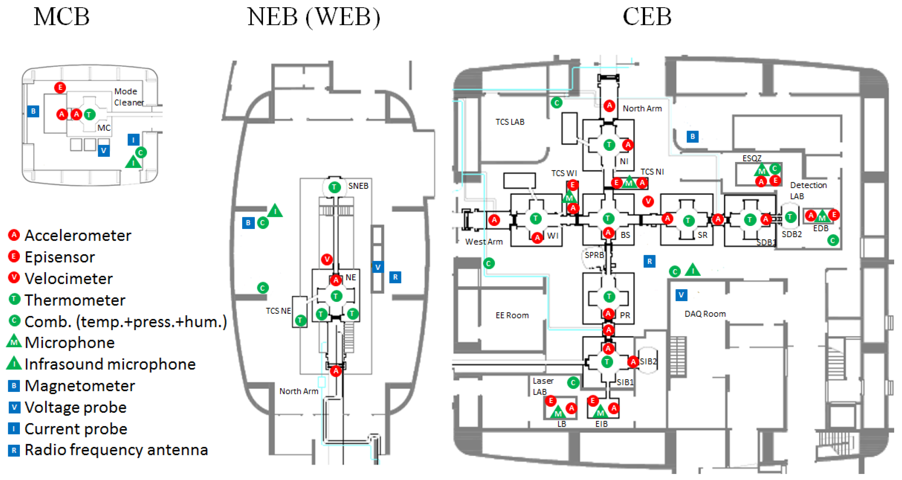
2. Environmental Monitors

The auxiliary monitors of the Virgo environment are essential for tracking sources and studying their influences. A distributed network of environmental probes was initially setup for Virgo [23] and, subsequently, expanded and enhanced for Advanced Virgo. In Figure 2, we show the current layout of sensors deployed in the central building, the input mode cleaner building, and the two buildings at the end of the North and West arms [24]. Other monitored locations are: the laser clean room hosting the in-air (i.e., at ordinary atmospheric pressure) benches carrying the laser source and input optics; the detection clean room hosting the in-vacuum suspended bench with the readout photodiode and the in-air bench for squeezed light injection; and a few electronic rooms. There are two categories of sensors: fast sensors, sampled at 1 kHz to 20 kHz according to the probe operating bandwidth, and slow sensors, which were sampled at 1 Hz. Table 1 provides a list of the sensors in use.
Fast sensors (∼150 probes) are magnetometers, radio frequency (RF) receivers, accelerometers, seismometers, microphones, power line voltage monitors, and current sensors. They continuously monitor the ambient noise close to the detector at frequencies up to 10 kHz. These sensors are low noise devices with enhanced low frequency response and they are positioned close to potential noise coupling sites. All of the external optical benches, which are prone to acoustically driven vibrations and thermal fluctuations, are monitored with one low frequency tri-axial accelerometer, one high frequency accelerometer, one microphone, and one temperature probe. In Advanced Virgo, we have added accelerometers in order to improve the monitoring of locations prone to scattered light coupling, such as vacuum chambers, vacuum separating windows, and cryogenic traps. Experimental halls noise is monitored from 0.1 Hz to 10 kHz with tri-axial seismometers, magnetometers, and new infrasound microphones.
Slow sensors are temperature, humidity, and air pressure probes, positioned in several sensitive locations in the experimental halls, clean rooms, electronic rooms, and along in-vacuum suspensions. These are approximately 300 probes. In addition, we monitor several service devices of the detector infrastructure, like air cleaning and conditioning, water pumps, chillers, illumination. The primary use of these monitors is in the Detector Monitoring System [25] for issuing safety alerts, but they are also often used to correlate devices operation with non-stationary disturbances. New monitors have been added during the O3 preparation phase and, presently, there are approximately 150 probes, including: illumination sensors, ambient over-pressure, air and water temperature and pressure, air and water flux, power monitors, and particle dust counters. The readout electronics of these monitors adopted in the initial Virgo was found to produce electromagnetic disturbances in the form of a comb of narrow equally-spaced lines associated to the timed communication data packets [26]. It has been replaced with a silent custom solution.
Advanced Virgo also has geophysical environmental monitors: one cosmic ray detector, one weather station, and one lightning sensor. One recent addition is two very low noise magnetometers (Metronix, mod. MFS-06e) that we installed at approximately one hundred meter distance from the central building with the purpose of sensing Schumann’s global magnetic field and electromagnetic noise transients correlated among distant interferometers [27,28].

3. Environmental Noise Couplings and Sources

In the initial Virgo, a major issue was noise due to light back scattering from vibrating surfaces on in-air and not seismically isolated optical benches [29,30]. In Advanced Virgo, most auxiliary optical benches have been suspended in light vacuum with residual gas pressure of ≈1 mbar [15]. This allows to reduce their displacement noise with respect to ground by 5 to 7 orders of magnitude at 10 Hz and provides acoustic isolation. In addition, each bench position is actively controlled to minimize its motion with respect to the main optics. Despite all of this, scattered light noise has been a major issue for both Virgo and LIGO during O3 [31,32,33,34]. In Section 5.1, we describe some scattered light noise investigations at Virgo during O3.
Advanced Virgo adopts a coil-magnet actuation system to control the angular and longitudinal position of the test masses. Four little magnets are glued on the back-side of each TM mirror in anti-parallel cross configuration in order to reduce the total magnetic moment [9,35].
Ambient magnetic fields induce eddy currents in the metallic structure surrounding the TM, which, in turn, warp the field and produce magnetic gradients. Magnetic fields and magnetic gradients couple to the mirror magnets, thus exerting a displacement force. The AdV new payload structure has been designed to reduce eddy currents, and its coupling with ambient magnetic fields was validated prior to assembling with simulations and measurements [35].
In Advanced Virgo, we have significantly reduced the ambient magnetic field in proximity of the TM mirrors vacuum chambers [36]. The main actions consisted of: (i) rerouting electric cables at further distance from chambers; (ii) using mains cables with twisted hot and neutral wires in the chamber proximity; and, (iii) replacing several step-down power supplies with toroidal shaped core types for the reduction of stray magnetic field. Despite these mitigation actions, during O3, we have faced residual magnetic noise coupling and sources, which we discuss in Section 5.2.
Among anthropogenic sources of noise, close-by flying vehicles (helicopters, airplanes) are a long lasting problem [37]. Air pressure waves from the rotor blades induce low frequency vibrations, usually in the range 10–150 Hz, in the experimental buildings walls and all their content. Scattered light noise paths can be excited. This was still a potential noise issue before O3, as we demonstrated with fly-over tests that were performed in collaboration with the italian 46th air brigade [38]. Just before O3 started, an agreement signed with the air force authorities enforced no-fly zones within cylindrical volumes of 600 m radius and height around the three Virgo vertices.
The majority of noise sources are part of the detector facility infrastructure, like ventilation systems and vacuum devices, or electronics, like power supplies, data and communication lines. Electrical devices using pulse-width-modulation (PWM) technique to regulate the delivered power produce amplitude modulation and, thus, spectral side-band noise of the mains frequency (50 Hz in Europe) or harmonics. We have replaced PWM heaters used to melt liquid Nitrogen condensation, which were producing 10 Hz magnetic combs, with variac regulated devices. Noise from other devices of this kind, like chillers used to cool down lasers and beam dumpers, or laser beam profilers is discussed in Section 5.4.

4. Noise Hunting Methods

Noise hunting is defined as the process of identifying noise sources and coupling paths to the interferometer, and pursuing a mitigation of their effects. Noise hunting makes use of specific data analysis and experimental methods that are described below.

4.1. Data Mining

Data mining is usually the first step. The Virgo and LIGO collaborations have developed several tools for monitoring and identifying noise features in the gravitational-wave signal (referred to as Hrec) and all of the auxiliary channels [39,40]. Here, we address the tools that are used for environmental noise hunting.
The search often starts from the careful inspection of noise features in the reconstructed strain signal. The time-frequency plots (spectrograms) that we automatically compute hourly and archive are extremely helpful. Typically, we look for the onset (or modification) of spectral noise features, like lines (monochromatic peaks) or bumps. This sometimes happens in coincidence with actions carried out on site and considered to be harmless, like turning on or modifying the operation set point of devices or detector components. Consequently, when we find unexpected features, we usually first look for possible coincident actions made on the experiment and reported on the Virgo electronic logbook [41].
We then search for correlated noise features in other channels, specifically the environmental ones. The most efficient approach is the so-called brute-force or exhaustive search. It consists in blindly estimating the correlation between Hrec and all of the auxiliary signals (thousands) used for the detector monitoring and control. For this purpose, data analysis tools have been developed looking for either linear or, more challenging, non-linear noise. An example of a linear noise search tool is BruCo [42,43], which computes brute-force coherence for Hrec with the auxiliary channels and outputs a ranked list of the most coherent signals at each frequency bin.
Noise with a periodicity in amplitude or frequency is often correlated with the operation cycle of infrastructure devices or with ambient temperatures. In this case, a brute-force correlation analysis with the slow monitors helps in pinpointing the noise source. Tools, like Buffalo [44] and NonNA [45], are used for this purpose.
Uncorrelated sources can sum and show up in Hrec at their beating frequency. MONET [46] is a tool that is dedicated to this search and during O3 it could spot beatings between slow residual angular drifts of suspended optics and detector calibration lines, violin modes, and mains harmonics [47].
Another category of non-linear noise is scattered light. It often produces typical spectral features in Hrec, like bumps and arches or shelves, which help in recognizing and tracking it down [29,31,48]. We show examples in Section 5.1.

4.2. Experimental Methods

Following the hints collected in the data mining step, a set of subsequent experimental actions is needed in order to better understand and pursue the mitigation of each noise source. Three experimental investigation methods are the mostly used: sniffing, switch off tests, and noise injections.
In the sniffing process, we use a set of portable magnetic, seismic, and acoustic probes (see Table 2) to inspect the experimental areas. With auxiliary sensors placed in the proximity of the suspected offender, we scrutinize a number of devices looking for the specific noise “signature” (frequency pattern) identified in the data mining step. One example during O3 was the localization of the source of the main sideband noise. We discuss it in Section 5.4.
The number of noisy devices is so large that, sometimes, the best strategy for finding a source is to perform selective switch off of suspected candidates, and observe whether the noise disappears from the gravitational-wave signal. As we discuss in Section 5.1, during O3, the temporary turn off of one air conditioning machine significantly reduced a number of structures in the amplitude spectral density (ASD) of the residual strain. In that eventuality, we further investigated the devices in that area. A lesson we learned is that “devices that are not strictly needed should stay off”. We provide an example in Section 5.5. For this reason, we have plugged several seldomly used devices on remote controllable mains sockets.
The last method we mention is noise injections. The noise injection technique is well known in the GW detector community [4,29,36,49]. The aim is to produce controlled and localized enhancements of the detector ambient noise in order to have a sizeable effect in the gravitational-wave signal allowing for the measurement of a noise coupling function. For this purpose, we use dedicated loudspeakers (acoustic injections), coils (magnetic injection), RF transmitting antennas (RF injections), and shakers (vibration injections). Main injection tools are listed in Table 2. These devices are conveniently driven with sets of sine waves (which allow to generate high intensity stimuli) or white/band-limited signals (that allow to span all frequency bins without blind spots). Subsequently, we use these coupling functions to compute the contribution to Hrec of the quiet ambient noise level (i.e., in absence of injected stimuli) named noise projection, and evaluate how critical it actually is. A plot of noise projections as compared to strain ASD is what we call a noise budget. We provide an example of noise injections and projections in Section 5.2.
Noise injections are also used for the hunt of specific noise structures in the gravitational-wave signal. In this case, more localized stimuli are generated, for example, with the use of a small portable bluetooth shaker or impact hammer actuating on a vacuum chamber, a bench or single optics. The frequency content of the stimulus is adjusted to match that of the target. The aim in this case is to excite the target noise, so as to establish a cause-effect relationship and pinpoint the offender or the coupling path. Section 5.1 describes examples.

5. O3 Noise Hunting

In this section, we describe the most relevant environmental noise search and mitigation actions performed in Advanced Virgo during the commissioning before and throughout the O3 observing run.

5.1. Scattered Light Noise Studies

A small fraction of the laser light circulating in the interferometer can be scattered off by any illuminated surface and, if not blocked, it might re-enter the main beam path adding a noise modulated by the motion of the scattering surface. Scattered light (SL) noise has been known for long [50], but it is particularly striking for the last generation of GW interferometers, which have very large circulating light power.
The model of the strain noise associated to light scattering by a surface displacing as x ( t ) is [51]:
n s c = C · K ϕ ( f ) · F sin 4 π λ x ( t ) + K δ P / P ( f ) · F cos 4 π λ x ( t )
where we indicated with F the Fourier transform, with λ = 1064 nm the laser wavelength, with K ϕ ( f ) and K δ P / P ( f ) , respectively, the transfer function from phase and amplitude noise to the detector measured strain, and with C a coupling constant that depends on the fraction of light re-coupling to the interferometer main beam. The K transfer functions depend on the micrometric position of the scattering source inside the interferometer and they are evaluated with an optical model of the interferometer, like Optickle [52]. The coupling constant C is estimated by a fit of the model to the measured data.
Spotting the presence of SL noise is not an easy task, primarily because it is non-linear and no coherence or very poor coherence with witness sensors is expected. Typical evidences of SL are spectral noise features, such as bumps in photodiode signals, which are non-stationary in time, with a typical timescale of a few hours. Bumps width typically increases with the level of microseismic noise. The amplitude of bumps can change from lock-to-lock, depending on the global interferometer alignment.
During O3, we used two experimental methods to test whether scattered light noise was impacting the sensitivity or was very close to do so: (1) switch off of heating, ventilation, and air conditioning (HVAC) systems; and, (2) enhance vibration noise of specific parts by means of shakers or loudspeakers. In the following, we illustrate some applications.
Seven air handling units are in continuous operation site-wide for the purpose of temperature control and dust decontamination of experimental areas. Clean laboratories have their dedicated unit with the addition of water chillers, heaters, and circulation pumps. These devices produce broadband acoustic noise that extend from 1 Hz to 100 Hz and monochromatic seismic-acoustic disturbances at fans and at engines rotation frequencies (10–30 Hz range). Air conditioners can be temporarily turned off for periods of 10 to 60 min., depending on the experimental area, without significantly affecting the interferometer operation.
One sequential switch off of all Virgo HVAC units was performed on 19 April 2019, and it lasted about 40 min. before restoring the initial condition. The effect was in real time visible in the BNS range online monitor (Figure 3a). Hrec noise reduced significantly below 30 Hz (Figure 3b). The time of the noise reduction could be correlated with the turning off of the HVAC unit serving the detection clean room. On 27 October 2019, a similar sequential switch off highlighted a new issue. The noise bumps at 20 Hz and 40 Hz in the strain ASD turned out to be correlated with the acoustic noise inside the laser clean room. Of course, air conditioners could not be kept off, but the tests provided useful hints. Subsequently, the investigation proceeded with techniques that permitted a more precise localization of the scatterer.
In the case of the laser clean room, the suspect fell onto the laser optical bench, which is in-air and it does not benefit from any seismic isolation. In fact, by examining the signal of the seismic sensor on the bench we found a significantly large (≈ 10 8 m/ Hz ) horizontal motion at about 20 Hz, which is a mechanical mode of the table (Figure 4a). This frequency matched that of a bump in the spectrum of the power recycling cavity length signal (PRCL), as shown by the blue line in Figure 4b.
We proceeded with applying a controlled vibration to the bench. For this purpose, we used one commercial shaker that was attached to one of the bench legs and loaded with a reaction mass. By applying a 20 Hz sinusoidal excitation, we managed to enhance the bench motion at the resonance by a factor ten. At the same time bumps at 20 Hz and harmonics grew in the PRCL spectrum.
These bumps can be reproduced by a simplified version of the scattered light model of Equation (1), as demonstrated in Figure 4b. In this case, the model is used to estimate not the strain noise but the PRCL noise due to scattered light. We used for x ( t ) the horizontal bench displacement measured by the seismic sensor. The scale factor C is determined by best matching the model (yellow curve in Figure 4b) and the data measured during injection (red curve in Figure 4b). The obtained value is C = 8 × 10 6 . The simplified model consisted in assuming unitary phase and amplitude noise transfer functions. For a thorough understanding of the noise path, the K ϕ and K δ P / P functions should be estimated and applied. Despite this simplification, the reasonable match between the data and model was sufficient to localize the source in the laser bench. In Figure 4b, the green curve also shows that the same model applied to the quiet data (i.e., in the absence of external stimuli) roughly explains the residual PRCL bumps noise.
An investigation followed, which identified and properly dumped stray beams on the bench. We aim to reduce the bench motion at 20 Hz adopting passive resonant dampers and diverting the clean air flux from the bench in order to further mitigate the noise.
The scattered light issue inside the detection clean room has been followed up with acoustic injections. We injected broadband 20–1000 Hz noise with one 18-inch sub-woofer inside the clean room. We injected increasing levels of noise and found that a little enhancement of sound level in the room was sufficient for stimulating the rise of a noise bump between 46 and 50 Hz in the strain ASD, as shown by the blue curve in the top panel of Figure 5. The same sound injection was repeated after having blocked the pick-off beam from the interferometer at the entrance of the squeezer bench, so that no laser light was present on the bench [12]. In this condition, even with a larger acoustic injection, the noise bump between 46 and 50 Hz was sensibly reduced and the injected noise did not produce any additional contribution in Hrec, as reported by the black curve in the top panel of Figure 5. This meant that the scattering source had to be located on the bench itself. Further investigations [34] have identified the scattering that occurred in some components installed on the bench, which, during O3, was placed in-air and rested on the ground. The coupling of this noise to Hrec was finally made negligible by optimizing the beam alignment on the bench.

5.2. Electromagnetic Noise Injections

We describe two applications of the aforementioned (Section 4.2) technique of noise injections. The first application is a far-field electromagnetic noise injection with the purpose of measuring the detector coupling to ambient magnetic and radio frequency fields and then estimate their noise contribution to the O3 residual strain noise. The second application is a near-field magnetic injection with the purpose of localizing an anomalous coupling to magnetic fields within the central area.
Monitoring magnetic noise coupling to the detector is also of interest for the stochastic GW search, where global magnetic fields (e.g., Schumann’s resonances [53,54]) can limit the sensitivity to searches of GW signals that are correlated over multiple detectors [27,28]. On a weekly basis, far-field magnetic injections were performed during O3 in order to monitor variations in the magnetic coupling function for far field sources1.
The setup consists of one coil (Table 2) that was placed inside the experimental area in the farthest possible location from all interferometer components [55]. The maximal current was 3 A, limited by the driving amplifier. With this setup, we generated sinusoidal fields with frequencies in the range 10 Hz to 500 Hz and intensities of 0.2 nT to 2 nT within the central hall, in proximity of the interferometer sensitive parts. This injected field added to the preexisting ambient field, whose intensity (apart for mains) is 1 pT to 10 pT, depending on frequencies and away from electromagnetic (EM) sources.
Equation (2) gives the magnetic coupling function (CF), with Y and X being, respectively, Hrec and the witness sensor during the injection ( i n j ) or an adjacent time without injection ( b k g ):
C F ( f ) m e a s u r e d = Y i n j 2 ( f ) Y b k g 2 ( f ) X i n j 2 ( f ) X b k g 2 ( f ) , C F ( f ) u p p e r l i m i t = Y b k g ( f ) X i n j 2 ( f ) X b k g 2 ( f ) .
The witness sensor of the total magnetic field is the modulus of the magnetic field observed by the three perpendicularly orientated magnetometers. If the injected field results in an increase of the strain ASD of at least a factor 2, we claim to have measured the coupling, see the dots in Figure 6. Otherwise, we place an upper-limit on the CF under the additional condition that the witness sensor detects an effect of at least a factor of 10, as pointed out by stars in Figure 62.
An in-depth discussion on magnetic injections can be found in [36]. Here, we comment on the two most important features of the measured coupling function: the low frequency part (up to 100 Hz) with a declining slope and the high frequency part (above 100 Hz) with a rising slope. The low frequency part is dominated by the coupling of the ambient magnetic field to the small magnets that are attached to the back of each TM mirror and they are used to control the mirror position. The coupling to these magnets is known to decay as f 3 , where f is the frequency [36]. The measurements at NEB and WEB confirmed the expected behavior, while the magnetic coupling measured in CEB does not follow the same slope. Even if we do not have a complete explanation for this result, it is reasonable to ascribe the enhanced low frequency coupling to other noise sources that were triggered by the magnetic injection (e.g., scattered light). This mechanism is very likely in the complex environment of the central building.
In order to understand the origin of high frequency slope of the magnetic coupling function we performed a set of near-field magnetic injections. We probed several locations within the central hall using one small injection coil (Table 2). We fed the coil with one pair of sinusoidal signals with fixed amplitude (I) and frequency (f): one in the low frequency region below 100 Hz (we chose: f = 28 Hz, I = 3 A) and one in the high frequency region (we chose: f = 368 Hz, I = 0.3 A). In this condition, a ∼1 nT field is generated at a distance of a few meters from the coil. This is the same order of magnitude of the intensity that is generated in the far field injections. Therefore, using the small coil as a stimulus and looking at the induced effect in Hrec, we could pinpoint the source location with a distance accuracy of a few meters.
The low frequency stimulus (28 Hz, triangles) couples significantly to Hrec when approaching the test mass at the input of the North arm (NI), as illustrated in Figure 7. Indeed, this behaviour is expected for fields coupling to mirror magnets. Instead, the coupling of high frequency stimulus (368 Hz, circles) gets larger and larger approaching the output suspended bench (SDB1).
The described method does not allow for a quantitative assessment. However, it helped in identifying the most likely noise path responsible for the high frequency increase of coupling to ambient magnetic fields in the central experimental area. The noise path is: ambient magnetic fields shake the SDB1 bench acting on the coil-magnet actuators. The enhanced bench vibration increases the coupling of scattered light noise from the bench that we know is close to limit, and is actually limiting at a few frequencies, the O3 strain ASD in the 300–600 Hz range. As further proof, we injected broadband 10–1000 Hz noise with the small coil in proximity of the SDB1 vacuum chamber and we could reproduce similar strain noise structures as when a white noise signal is sent to the bench coil-magnet actuators.

5.3. Evaluation of Residual Magnetic Noise

Figure 8 reports the noise budget of ambient magnetic noise in the Virgo central area. In order to visualize the variability of the ambient fields, projections are computed while using percentile ASD of the ambient fields.
The noise budget provides information on the relevance of the ambient noise: if the projected noise is close to the strain ASD, it requires immediate attention; otherwise, it might become relevant as the detector sensitivity improves. If the noise is at least a factor ten below the target sensitivity it is expected to not contribute significantly and can be given little attention.
Examining Figure 8, we notice the noise estimate is quite low across most of the frequency band, except for some frequencies, where the 90th percentile (or even 50th percentile) has a predicted noise level, which is less than a factor of ten below the O3b strain noise.
Many of these peaks are located around the mains frequency (50 Hz) and harmonics. However, the effect at 50 Hz is mitigated by an active subtraction (Section 5.4). The two peaks at approximately 49.5 Hz an 50.5 Hz are linked to the MCB electric heater and limit the O3b sensitivity at those frequencies, see top panel of Figure 8. A probable pathway for this magnetic noise from the MCB to the CEB is an electric current flowing in the mode cleaner pipe.
If no actions are taken, then magnetic noise will be limiting the Virgo detector sensitivity at several frequencies in O4 and even more in O5, as seen in Figure 8. Four main activities are planned between O3 and O4 in order to minimize the impact of magnetic noise on future observing runs.
The first action to mitigate the magnetic noise from the MCB HVAC system presented in the CEB was already successfully completed during the last months. The MCB and CEB were sharing their low voltage mains circuit, each with three phases and a common neutral wire. In the case of an unbalance between the three phases, the neutral wire will be used as return for the unbalanced current. However, if this neutral wire has, somewhere, a connection to the protective earth, the unbalanced current will chose any low resistance connection, such as the MCB vacuum pipe. An insulating transformer has been placed to separate the neutral wires of the MCB and CEB. All of the magnetic noise known to originate from the MCB HVAC system disappeared from the CEB magnetometers after this action [56].
Secondly, new diaphragm baffles will be installed at SDB1 in order to reduce scattered light. This action aims to reduce the slope of the coupling function above 100 Hz.
Thirdly, alternatives are being investigated for vacuum-equipment near the test masses. During O3 noise hunting efforts, some pressure gauges were identified as a local source of magnetic fields. A temporary switch off reduced the local magnetic field up to 1 kHz, and partially removed 0.5 Hz and 5 Hz magnetic combs [57].
Finally, larger injection coils with a radius of a few meters will be build, so that we can inject broadband magnetic noise instead of the current discrete-frequency injections.

5.4. Mains and Sidebands

The frequency of the mains electrical system in Virgo is 50 Hz. A quite intense 50 Hz noise was affecting Hrec before O3. The path of this coupling was investigated. Various searching techniques were used, like switching off several components and verifying the electronics grounding. However, neither of these were successful. Eventually, the 50 Hz noise has been substantially removed with a feed forward control scheme. This control uses the voltage monitor of the uninterruptible power supply (UPS) of the central building and applies a longitudinal correction to West input mirror actuators. The control features a factor 10 3 suppression and no sensible noise re-injection, as illustrated in Figure 9a.
However, one residual noise was present in the interferometer strain signal as reported in the bottom panel of Figure 9b. The noise was shaped as symmetric peaks around 50 Hz, namely sidebands. The most pronounced being a pair of peaks that could be grouped in two families: ± 1.25 Hz with its double at ± 2.5 Hz, and ± 1.7 Hz with its double at ± 3.4 Hz and triple at ± 5.1 Hz.
This sideband noise is common in Virgo. It is typically associated to power controlled loads that cause periodic amplitude modulation of the mains. We experienced this noise from devices, such as water chillers or electrical heaters.
The coherence of sidebands with the UPS monitors and the magnetic and electric probes of the central building (spotted with the BruCo tool) indicated the EM origin of this disturbance, and the source being located in the central area. Moreover, it had to be a device component of the interferometer electronics infrastructure, which, at Virgo, is powered by an UPS system to guarantee continuity of operation. Indeed, further evidence emerged from the data of a site power outage on 4 June 2019, during which the noise from the sidebands did not disappear, proving that the offensive device was powered by the UPS.
We used a magnetic probe that was connected to a portable C h r o m e b o o k (a setup developed at KAGRA [7]) to sniff noise emissions of each electric switchboards within the central experimental area, while looking for the presence of the characteristic spectral peaks in the probe spectrum. The search led us to the switchboard in the thermal compensation system (TCS) area. Following the noise emissions along power cables, we ended-up at the two optical benches hosting the CO 2 lasers that were used to compensate the thermal lensing that was generated by the main laser beam in the North and West Input mirrors [13,58]. In particular, the 1.2 Hz sideband family originated from the West bench and 1.7 Hz family from the North bench. Finally, by selectively switching off devices on the benches, the source was identified in the infra-red laser beam profilers, one for each TCS bench, which have a variable load cycle of 0.8 s and 0.65 s, respectively. These devices have been installed on the CO 2 benches in order to monitor the heating pattern profiles. Given that their role is purely diagnostic, they can be kept off during the observing run mode and switched on upon need.
In Figure 9b, we show the magnetometer (top) located in proximity of the TCS bench and the strain ASD noise (bottom). The achieved reduction of upper sidebands at 51.2 Hz and 51.7 Hz is well visible in the Hrec signal after the switch-off of the beam profilers. Peaks in Hrec at frequencies below 50 Hz are not associated to sidebands, but they have different origin. They are examined in Section 5.5.

5.5. Charged Mirrors

In summer 2018, during the O3 preparation phase, several commissioning activities were carried out, while the interferometer remained unavailable for more than thirty consecutive days without the possibility of checking the noise impact of each single intervention. When the detector was finally recovered a new mysterious noise, with a spectral frequency dependence of 1/ f 2.5 , worsening of the detector sensitivity up to 100 Hz had appeared (the black curve in Figure 1).
LIGO had observed a disturbance of similar shape due to the coupling of noise produced by their electrostatic actuator drivers with the electrically charged TM mirror [59]. To see whether we were suffering from a similar problem, we first had to determine whether our TM mirrors were charged, and then identify the presumed source of electrostatic force on the mirror.
We devised a method that, operating from remote on the coil actuators, allows determining whether a TM mirror is electrically charged and, in case, extract a measure of the charge.
A signal, V i n j = V p e a k sin ( 2 π f t ) with frequency f, was applied at both ends of the actuation coils of the mirrors. The coil-charged mirror system can be modelled as a capacitor whose plates are the coil and the mirror face. The energy stored in the capacitor is given by E = [ C V m i r + V i n j 2 ] / 2 , with V m i r the electrostatic potential of the charged mirror and C = ε S / x , where ε , S, x are the dielectric constant, mirror surface, and distance between coil and mirror, respectively. The resulting force on the mirror is given by:
F = d E d x = 1 2 d C d x V m i r + V i n j 2 = 1 2 C x V m i r 2 + C x V m i r V i n j + 1 2 C x V i n j 2 .
The coil-mirror distance is x = d + Δ L , where d is the effective distance between the Virgo mirror and coil and Δ L = h L is the differential arms length, h is the gravitational strain, and L is the Virgo arm length. Being Δ L d and x d , the first term in brackets is static and it can be neglected.
The equation for motion of the mirror with mass m, for frequencies that are higher than the last suspension resonance, is: F = m a = m ω 2 Δ L . When comparing with the previous equation, we have two force contributions that depend on f and 2 f :
F f = m ω 2 h f L C d V m i r V i n j h f V m i r sin ( 2 π f t ) ,
F 2 f = m ω 2 h 2 f L 1 2 C d V i n j 2 h 2 f V p e a k 2 cos ( 4 π f t ) ,
where h f and h 2 f are the strain component at the injected frequency and at its first harmonic, respectively. The injected signal shows up in Hrec at double of its frequency (Equation (5)). If the mirror is charged ( V m i r 0 ), the injected signal also shows up at its fundamental frequency (Equation (4)). Moreover, being:
V m i r = h f h 2 f V i n j ,
the charge density on the mirror surface can be estimated:
σ = ε 0 d V m i r ,
with d = 10 mm. The relative sign of the charge is determined by the relative phase between h ( t ) and V i n j ( t ) measured with a transfer function. We stress that the method estimates the charge density value in the portion of the mirror surface in front of the actuation coil.
Each coil of each one of the four TM mirrors was tested in turn. All four test mass mirrors were found to be electrically charged with surface density values of the order of some tens of pC/cm 2 . The charge density that was measured in front of each coil of the same mirror typically had different magnitude and sign. This indicates that the charge is not uniformly distributed over the mirror dielectric surface. The mirror charging may have occurred just after the TM payloads installation before evacuating the vacuum chambers, and remained as such since then. We think the charging might have occurred when removing the mirror’s protection film or through accidental contact of the mirror surface with the safety peek stoppers.
Virgo TM actuator coils can exert an electrostatic force in case a common mode signal is present at both ends. To test this occurrence, we unplugged the actuator coils of one TM, while keeping the interferometer locked acting on the opposite TM. The 1 / f 2.5 noise reduced, proportionally to the number of coils disconnected at the same time. We found that the source of the common mode noise from the coils was the modified version of the coil driver board that had been installed in summer 2018. The new driver produced a common mode noise with a spectral shape of 1 / f , while the additional 1 / f 2 shape was due to the pendulum’s mechanical transfer function. The driver problem was fixed and the noise disappeared.
A second noise issue that was related to the mirrors charge was solved at the end of O3b period. An excess noise was present in the strain ASD between 40 Hz and 50 Hz, as shown by the blue curve in Figure 10. BruCo provided the first clue, highlighting a slight coherence with the magnetic probes in the west terminal building. Sniffing the area with a portable magnetometer gave a further indication that the source must have been located near the west end (WE) mirror chamber. However, neither the switching off of potential sources around the chamber (cooling fans, digital vacuum sensors) nor the addition of external stimuli (shaking the chamber, injecting magnetic field) revealed the mysterious noise.
Eventually, the event that led to the understanding and cure of the problem was to observe the noise temporarily reducing during a period of failure of one of the UPS devices. The mirror suspension control electronics, which is UPS powered, is a physical connection between the UPS mains line and the WE test mass. A selective disconnection test of these electronic modules allowed us to identify the noise path. We found that the module power supply neutral wire was producing a common mode noise into the signal wires that drive the stepper motors, used for the positioning and balancing of the WE test mass suspension. Stepper motor wires run tens of meters inside the vacuum chamber in the same bundle together with the mirror coil actuators’s wires. The noise was coupling capacitively to coil actuators wires and, once at the coils, it exerted an electrostatic force on the electrically charged mirror. As a test, we were able to replicate the noise in Hrec by injecting a synthesized signal between the ground and the neutral wire of the stepper motors power supply. Given that these motors are not used during operation, they were left disconnected and the noise disappeared from Hrec.
Following the experience of LIGO, where the mirrors are routinely discharged, we are now studying a mirror discharging system.

6. Conclusions and Future Perspectives

The study of environmental disturbances was a major topic of investigation during the setup phase of the Advanced Virgo detector and throughout the O3 scientific run. The network of probes monitoring the detector environment and the operation of the infrastructure monitors has been improved and extended with respect to the initial Virgo. Experimental methods and software tools for data monitoring and extended correlation studies have been fruitfully applied in the noise search. This work contributed to gaining a better understanding of noise sources and coupling paths, which is useful in reaching the 60 Mpc goal. Several environmental sources affecting the Advanced Virgo interferometer have been addressed and cured. New unexpected paths have been found, such as the electrostatic noise coupling to the residual charge on TM mirrors. The residual unexplained noise has the characteristics of scattered light noise.
Due to the COVID-19 pandemic, the commissioning activities planned to address these issues will be carried out at the end of the installation of the experiment upgrades, named AdV+. The target of AdV+ is to increase the BNS range by about a factor 2. The detector upgrade started in June 2020. It consists of implementing new optical cavities, such as the signal recycling cavity and the filter cavity for frequency dependent squeezing, and a new auxiliary green light source with the associated optical system. The environmental probe network is being upgraded in order to monitor these new detector systems. Additionally, central and terminal buildings are being instrumented with seismometer arrays for Newtonian noise cancellation. New hardware for noise injections will be installed, such as low frequency vibration exciters for the investigation of scattered light and large coils for more accurate assessment of ambient EM noise coupling. Remote control and automation of the injection procedure is being pursued. Profiting from the detector downtime, some identified problems in the detector infrastructure are being cured, like residual vibration noise from air conditioning devices, and electromagnetic noise from the experimental power grid. The implementation of a system for periodic discharging of mirror test masses is under study.
The interferometer network plans a new joined data taking, also including KAGRA, the O4 observation run, which is currently planned for 2022. Environmental monitors, experimental techniques, and tools described in this paper will be used for assessing the infrastructure performance of the new detector and hunt for unexpected couplings.

Author Contributions

Writing–original draft preparation, I.F., F.P., M.C.T., K.J., C.K., A.M.-V., A.R.R.; writing–review and editing, M.C.T., I.F., K.J., T.W., A.R.R.; investigation, V.B., A.C., M.C., R.D.R., C.D.R., F.D.R., I.N., A.P., B.P., P.R., N.S., R.S., T.W. All authors have read and agreed to the published version of the manuscript.

Funding

This work was supported by the following fundings: European Gravitational Observatory; TEAM/2016-3/19 grant from the Foundation for Polish Science; FWO-Vlaanderen via grant number 11C5720N; Spanish MINECO under the grants SEV-2016-0588 and PGC2018-101858-B-I00; JSPS Core-to-Core Program Advanced Research Networks; JSPS KAKENHI Grant Number 19J01299 and Polish National Science Centre grant Harmonia 2017/26/M/ST9/00978. MC is supported by IRAP AstroCeNT funded by FNP from ERDF.

Acknowledgments

The authors thank their colleagues of the Virgo Collaboration and the staff of the EGO laboratory. Authors are also grateful to Vincenzo Dattilo, Diego Passuello, Bas Swinkels and Matteo Tacca for fruitful discussions and constant support; Robert Schofield for being an undisputed reference in this field; Tomasz Bulik, Mario Martinez and Takaaki Yokozawa for having entrusted us with their brilliant young collaborators; Giovanni Losurdo and Geppo Cagnoli for their advices in the charged mirror measurement.

Conflicts of Interest

The authors declare no conflict of interest.

Abbreviations

ASDAmplitude Spectral Density
BBHBinary Black Hole
BNSBinary Neutron Star
CEBCEntral Building
CFCoupling Function
DACDigital to Analog Converter
EMElectroMagnetic
GWGravitational Wave
Hrecreconstructed gravitational strain signal
HVACHeating Ventilation and Air Conditioning
MCBMode Cleaner Building
NEBNorth End Building
PRCLPower Recycling Cavity Length
RFRadio Frequency
SDB1Suspended Detection Bench 1
SLScattered Light
TCSThermal Compensation System
TMTest Mass
UPSUninterruptible Power Supply
WEBWest End Building

References

  1. Abbott, B.P.; Abbott, R.; Abbott, T.D.; Abernathy, M.R.; Acernese, F.; Ackley, K.; Adams, C.; Adams, T.; Addesso, P.; Adhikari, R.X.; et al. Observation of Gravitational Waves from a Binary Black Hole Merger. Phys. Rev. Lett. 2016, 116, 061102. [Google Scholar] [CrossRef] [PubMed]
  2. Effler, A.; Schofield, R.M.S.; Frolov, V.V.; González, G.; Kawabe, K.; Smith, J.R.; Birch, J.; McCarthy, R. Environmental Influences on the LIGO Gravitational Wave Detectors during the 6th Science Run. Class. Quantum Gravity 2015, 32, 3. [Google Scholar] [CrossRef] [Green Version]
  3. Covas, P.B.; Effler, A.; Goetz, E.; Meyers, P.M.; Neunzert, A.; Oliver, M.; Pearlstone, B.L.; Roma, V.J.; Schofield, R.M.S.; Adya, V.B.; et al. Identification and mitigation of narrow spectral artifacts that degrade searches for persistent gravitational waves in the first two observing runs of Advanced LIGO. Phys. Rev. D 2018, 97, 082002. [Google Scholar] [CrossRef] [Green Version]
  4. Acernese, F.; Amico, P.; Al-Shourbagy, M.; Aoudia, S.; Avino, S.; Babusci, D.; Ballardin, G.; Barillé, R.; Barone, F.; Barsotti, L.; et al. A first study of environmental noise coupling to the Virgo interferometer. Class. Quantum Gravity 2005, 22, S1069–S1077. [Google Scholar] [CrossRef] [Green Version]
  5. Acernese, F.; Alshourbagy, M.; Amico, P.; Antonucci, F.; Aoudia, S.; Arun, K.G.; Astone, P.; Avino, S.; Baggio, L.; Ballardin, G.; et al. Noise studies during the first Virgo science run and after. Class. Quantum Gravity 2008, 25, 184003. [Google Scholar] [CrossRef]
  6. Acernese, F.; Amico, P.; Alshourbagy, M.; Antonucci, F.; Aoudia, S.; Astone, P.; Avino, S.; Babusci, D.; Ballardin, G.; Barone, F.; et al. Analysis of noise lines in the Virgo C7 data. Class. Quantum Gravity 2007, 24, S433–S443. [Google Scholar] [CrossRef]
  7. Akutsu, T.; Ando, M.; Arai, K.; Arai, Y.; Araki, S.; Araya, A.; Aritomi, N.; Asada, H.; Aso, Y.; Bae, S.; et al. Overview of KAGRA: Calibration, Detector Characterization, Physical Environmental Monitors, and the Geophysics Interferometer. arXiv 2020, arXiv:2009.09305. [Google Scholar]
  8. LIGO Scientific Collaboration. Advanced LIGO. Class. Quantum Gravity 2015, 32, 074001. [Google Scholar] [CrossRef]
  9. Virgo Collaboration. Advanced Virgo: A second-generation interferometric gravitational wave detector. Class. Quantum Gravity 2014, 32, 024001. [Google Scholar] [CrossRef] [Green Version]
  10. Affeldt, C.; Danzmann, K.; Dooley, K.L.; Grote, H.; Hewitson, M.; Hild, S.; Hough, J.; Leong, J.; Lu¨ck, H.; Prijatelj, M.; et al. Advanced techniques in GEO 600. Class. Quantum Gravity 2014, 31, 224002. [Google Scholar] [CrossRef]
  11. Akutsu, T.; Ando, M.; Arai, K.; Arai, Y.; Araki, S.; Araya, A.; Aritomi, N.; Asada, H.; Aso, Y.; Atsuta, S.; et al. First cryogenic test operation of underground km-scale gravitational-wave observatory KAGRA. Class. Quantum Gravity 2019, 36, 165008. [Google Scholar] [CrossRef] [Green Version]
  12. Acernese, F.; Agathos, M.; Aiello, L.; Allocca, A.; Amato, A.; Ansoldi, S.; Antier, S.; Arène, M.; Arnaud, N.; Ascenzi, S.; et al. Increasing the Astrophysical Reach of the Advanced Virgo Detector via the Application of Squeezed Vacuum States of Light. Phys. Rev. Lett. 2019, 123, 231108. [Google Scholar] [CrossRef] [PubMed] [Green Version]
  13. Rocchi, A.; Coccia, E.; Fafone, V.; Malvezzi, V.; Minenkov, Y.; Sperandio, L. Thermal effects and their compensation in Advanced Virgo. J. Phys. Conf. Ser. 2012, 363, 012016. [Google Scholar] [CrossRef]
  14. Acernese, F.; Antonucci, F.; Aoudia, S.; Arun, K.G.; Astone, P.; Ballardin, G.; Barone, F.; Barsuglia, M.; Bauer, T.S.; Beker, M.G.; et al. Measurements of Superattenuator seismic isolation by Virgo interferometer. Astropart. Phys. 2010, 33, 182–189. [Google Scholar] [CrossRef] [Green Version]
  15. Van Heijningen, J.V.; Bertolini, A.; Hennes, E.; Beker, M.G.; Doets, M.; Bulten, H.J.; Agatsuma, K.; Sekiguchi, T.; Van den Brand, J.F.J. A multistage vibration isolation system for Advanced Virgo suspended optical benches. Class. Quantum Gravity 2019, 36, 7. [Google Scholar] [CrossRef]
  16. Gravitational-Wave Candidate Event Database. Available online: https://gracedb.ligo.org/superevents/public/O3/ (accessed on 4 December 2020).
  17. LIGO Scientific Collaboration and Virgo Collaboration. GWTC-2: Compact Binary Coalescences Observed by LIGO and Virgo During the First Half of the Third Observing Run. Available online: https://arxiv.org/abs/2010.14527 (accessed on 4 December 2020).
  18. LIGO Scientific Collaboration and Virgo Collaboration. GW190412: Observation of a binary-black-hole coalescence with asymmetric masses. Phys. Rev. D 2020, 102, 043015. [Google Scholar] [CrossRef]
  19. LIGO Scientific Collaboration and Virgo Collaboration. GW190425: Observation of a Compact Binary Coalescence with Total Mass ∼3.4 M. Astrophys. J. 2020, 892, L3. [Google Scholar] [CrossRef]
  20. LIGO Scientific Collaboration and Virgo Collaboration. GW190814: Gravitational Waves from the Coalescence of a 23 Solar Mass Black Hole with a 2.6 Solar Mass Compact Object. Astrophys. J. 2020, 896, L44. [Google Scholar] [CrossRef]
  21. LIGO Scientific Collaboration and Virgo Collaboration. GW190521: A Binary Black Hole Merger with a Total Mass of 150 M. Phys. Rev. Lett. 2020, 125, 101102. [Google Scholar] [CrossRef]
  22. LIGO Scientific Collaboration and Virgo Collaboration. Prospects for Observing and Localizing Gravitational-Wave Transients with Advanced LIGO, Advanced Virgo and KAGRA. Living Rev. Relativ. Vol. 2016, 19. [Google Scholar] [CrossRef] [Green Version]
  23. Barone, F.; De Rosa, R.; Eleuteri, A.; Milano, L.; Qipiani, K. The environmental monitoring system of VIRGO antenna for gravitational wave detection. IEEE Trans. Nucl. Sci. 2002, 49, 405–410. [Google Scholar] [CrossRef]
  24. De Rosa, R.; Fiori, I. AdV ENV Probe Maps (Fast and Slow Sensors). May 2019. Available online: https://tds.virgo-gw.eu/ql/?c=13976 (accessed on 4 December 2020).
  25. Berni, F.; Carbognani, F.; Dattilo, V.; Gherardini, F.; Hemming, G.; Verkindt, D. The Detector Monitoring System. May 2012. Available online: https://tds.virgo-gw.eu/ql/?c=9005 (accessed on 4 December 2020).
  26. Dattilo, V. Comb at 10.2782 Hz: Path and Source Identification. October 2011. Available online: https://logbook.virgo-gw.eu/virgo/?r=30429 (accessed on 4 December 2020).
  27. Coughlin, M.W.; Cirone, A.; Patrick, M.; Sho, A.; Boschi, V.; Chincarini, A.; Christensen, N.L.; De Rosa, R.; Effler, A.; Fiori, I.; et al. Measurement and subtraction of Schumann resonances at gravitational-wave interferometers. Phys. Rev. D 2018, 97, 102007. [Google Scholar] [CrossRef] [Green Version]
  28. Kowalska-Leszczynska, I.; Bizouard, M.A.; Tomasz, B.; Nelson, C.; Michael, C.; Gołkowski, M.; Jerzy, K.; Kulak, A.; Mlynarczyk, J.; Florent, R.; et al. Globally coherent short duration magnetic field transients and their effect on ground based gravitational-wave detectors. Class. Quantum Gravity 2017, 34, 074002. [Google Scholar] [CrossRef] [Green Version]
  29. Accadia, T.; Acernese, F.; Antonucci, F.; Astone, P.; Ballardin, G.; Barone, F.; Barsuglia, M.; Bauer, T.S.; Beker, M.G.; Belletoile, A.; et al. Noise from scattered light in Virgo’s second science run data. Class. Quantum Gravity 2010, 27, 194011. [Google Scholar] [CrossRef]
  30. Canuel, B.; Fiori, I.; Marque, J.; Tournefier, E. Diffused Light Mitigation in Virgo and Constraints for Virgo+ and AdV. December 2009. Available online: https://tds.virgo-gw.eu/ql/?c=7118 (accessed on 4 December 2020).
  31. Soni, S.; Austin, C.; Effler, A.; Schofield, R.M.S.; Gonzalez, G.; Frolov, V.V.; Driggers, J.C.; Pele, A.; Urban, A.L.; Valdes, G.; et al. Reducing Scattered Light in LIGO’s Third Observing Run. arXiv 2020, arXiv:2007.14876. [Google Scholar]
  32. Was, M.; Gouaty, R.; Bonnand, R. End Benches Scattered Light Modeling and Subtraction in Advanced Virgo. arXiv 2020, arXiv:2011.03539v1. [Google Scholar]
  33. Schofield, R.; Nguyen, P.; Banagiri, S.; Austin, C.; Merfeld, K.; Effler, A.; Shoemaker, D.; Siddharth, S.; Helmling-Cornell, A.; Ball, M. August 2019 PEM Update and New Techniques for Localizing Scattering. August 2019. Available online: https://dcc.ligo.org/LIGO-G1901683/public (accessed on 4 December 2020).
  34. Eisenmann, M.; Flaminio, R.; Gouaty, R. The ESQB Mechanical Resonances Analysis. July 2020. Available online: https://tds.virgo-gw.eu/ql/?c=15790 (accessed on 4 December 2020).
  35. Cirone, A.; Chincarini, A.; Neri, M.; Farinon, S.; Gemme, G.; Fiori, I.; Paoletti, F.; Majorana, E.; Puppo, P.; Rapagnani, P.; et al. Magnetic coupling to the advanced Virgo payloads and its impact on the low frequency sensitivity. Rev. Sci. 2018, 89, 114501. [Google Scholar] [CrossRef]
  36. Cirone, A.; Fiori, I.; Paoletti, F.; Perez, M.M.; Rodríguez, A.R.; Swinkels, B.L.; Vazquez, A.M.; Gemme, G.; Chincarini, A. Investigation of magnetic noise in advanced Virgo. Class. Quantum Gravity 2019, 36, 225004. [Google Scholar] [CrossRef] [Green Version]
  37. LIGO Scientific Collaboration; Virgo Collaboration; Coughlin, M.W. Identification of long-duration noise transients in LIGO and Virgo. Class. Quantum Gravity 2011, 28, 235008. [Google Scholar] [CrossRef] [Green Version]
  38. Boschi, V.; 46th Airbrigade; Fiori, I.; Mantovani, M.; Menzione, N.; Paoletti, F.; Pillant, G.; Tringali, M.C. C130J Flyover Tests. January 2019. Available online: https://logbook.virgo-gw.eu/virgo/?r=44268 (accessed on 4 December 2020).
  39. Aasi, J.; Abadie, J.; Abbott, B.P.; Abbott, R.; Abbott, T.; Abernathy, M.R.; Accadia, T.; Acernese, F.; Adams, C.; Aams, T.; et al. The characterization of Virgo data and its impact on gravitational-wave searches. Class. Quantum Gravity 2012, 29. [Google Scholar] [CrossRef]
  40. Aasi, J.; Abadie, J.; Abbott, B.P.; Abbott, R.; Abbott, T.; Abernathy, M.R.; Accadia, T.; Acernese, F.; Adams, C.; Aams, T.; et al. Characterization of the LIGO detectors during their sixth science run. Class. Quantum Gravity 2015, 32. [Google Scholar] [CrossRef] [Green Version]
  41. Virgo Electronic Logbook. Available online: https://logbook.virgo-gw.eu/virgo/ (accessed on 4 December 2020).
  42. Vajente, G. BRUte Force COherence. May 2017. Available online: https://github.com/gw-pem/bruco (accessed on 4 December 2020).
  43. Vajente, G. Analysis of Sensitivity and Noise Sources for the Virgo Gravitational Wave Interferometer. Ph.D. Thesis, Scuola Normale Superiore, Pisa, Italy, 2008. Chapter 8. [Google Scholar]
  44. Swinkels, B. Brute Force Correlation of Drifting Lines. June 2018. Available online: https://tds.virgo-gw.eu/ql/?c=13316 (accessed on 4 December 2020).
  45. Di Renzo, F. NonNA: A Non-Stationary Noise Analysis Tool. March 2019. Available online: https://tds.virgo-gw.eu/ql/?c=15883 (accessed on 4 December 2020).
  46. Patricelli, B.; Cella, G. Tools for Modulated Noise Study. June 2019. Available online: https://tds.virgo-gw.eu/ql/?c=14409 (accessed on 4 December 2020).
  47. Wąs, M.; Patricelli, B. Range Variations and Subtraction Efficiency. December 2019. Available online: https://logbook.virgo-gw.eu/virgo/?r=47852 (accessed on 4 December 2020).
  48. Marque, J.; Vajente, G. Stray Light Issues. In Advanced Interferometers and the Search for Gravitational Waves: Lectures from the First VESF School on Advanced Detectors for Gravitational Waves; Astrophysics and Space Science Library; Springer International Publishing: Basel, Switzerland, 2014; pp. 275–290. [Google Scholar]
  49. Kruck, J.; Schofield, R. Environmental Monitoring: Coupling Function Calculator. August 2016. Available online: https://dcc.ligo.org/LIGO-T1600387/public (accessed on 4 December 2020).
  50. Billing, H.; Maischberger, K.; Rudiger, A.; Schilling, R.; L Schnupp, L.; Winkler, W. An argon laser interferometer for the detection of gravitational radiation. J. Phys. E Sci. Instrum. 1979, 12, 1043–1050. [Google Scholar] [CrossRef]
  51. Canuel, B.; Genin, E.; Vajente, G.; Marque, J. Displacement noise from back scattering and specular reflection of input optics in advanced gravitational wave detectors. Opt. Express 2013, 21, 10546. [Google Scholar] [CrossRef] [PubMed]
  52. Evans, M. Optickle. November 2020. Available online: https://dcc.ligo.org/T070260/public (accessed on 4 December 2020).
  53. Schumann, W. Über die strahlungslosen Eigenschwingungen einer leitenden Kugel die von einer Luftschicht und einer Ionosphärenhülle umgeben ist. Z. Naturforschung Teil A 1952, 7, 149. [Google Scholar] [CrossRef]
  54. Sentman, D.D. Schumann Resonances. In Handbook of Atmospheric Electrodynamics; Volland, H., Ed.; CRC Press: Boca Raton, FL, USA, 1995; Volume I, Chapter 11. [Google Scholar]
  55. Fiori, I.; Bersanetti, D.; Cirone, A. Magnetic Injections CEB. July 2017. Available online: https://logbook.virgo-gw.eu/virgo/?r=38369 (accessed on 4 December 2020).
  56. Paoletti, F.; Fiori, I.; Soldani, D.; D’Andrea, M. TEST: Separating CEB and MCB Mains Lines, and Reducing the Unwanted Coupling between Them (50 Hz HVAC Sidebands in Hrec). November 2019. Available online: https://logbook.virgo-gw.eu/virgo/?r=49102 (accessed on 4 December 2020).
  57. Fiori, I.; De Rossi, C.; Paoletti, F. Hunting for 5 Hz Comb and the Higher Magnetic Fields Close to WE Chamber. November 2019. Available online: https://logbook.virgo-gw.eu/virgo/?r=47617 (accessed on 4 December 2020).
  58. Nardecchia, I.; Aiello, L.; Cesarini, E.; Lumaca, D.; Fafone, V.; Maggiore, R.; Lorenzini, M.; Minenkov, Y.; Rocchi, A. Integrated dynamical thermal compensation techniques for Advanced Virgo. In Proceedings of the 2nd GRavitational-Waves Science and Technology Symposium (GRASS 2019), Padova, Italy, 17–18 October 2019. [Google Scholar] [CrossRef]
  59. Martynov, D. 1/f2 Noise. October 2016. Available online: https://alog.ligo-la.caltech.edu/aLOG/index.php?callRep=28644 (accessed on 4 December 2020).
1.
The ideal condition would be that of generating a uniform field across the whole interferometer and the witness sensors. The best practical approximation that we could do consisted of one injection coil that was placed in one corner of the experimental halls and witness magnetometers centrally located with respect to the potentially sensitive components.
2.
We also evaluated the impact of ambient EM fields at frequencies within 10 kHz from the Virgo laser modulation frequencies ( F m o d ) 6 MHz, 8 MHz, and 56 MHz. These fields might couple to electronics contaminating the demodulated photodiode signals used for the angular and longitudinal controls of the interferometer. In this case, we used one transmitting antenna (6 m long vertical whip) positioned in proximity of the central building to broadcast 20 kHz-span sweep signals that were centered at each F m o d . This antenna was fed with a broadband power radio frequency amplifier set for an output of about 10 W. The contribution of the ambient radio frequency background was estimated to be more than one order of magnitude below the current Virgo sensitivity.
Figure 1. Amplitude spectral density of residual strain noise for Advanced Virgo in October 2018 (black), best of O3a (blue), best of O3b (red), and O3 observing scenario (green belt). The binary neutron stars (BNS) range is quoted as the average distance to which a signal generated by a BNS system with 1.4 M -1.4 M could be detected.
Galaxies 08 00082 g001
Figure 2. Virgo environmental probes. Top left: mode cleaner building (MCB). Middle: North end building (NEB). West end building (WEB) is identical. Right: central building (CEB).
Galaxies 08 00082 g002
Figure 3. Effect of turning off HVAC devices in binary neutron star range (a) and detector sensitivity (b). In (a), the black and purple dotted lines points out the beginning and ending of the switch off test, the red and green lines indicates the switching off of CEB hall and detection clean room units, respectively.
Galaxies 08 00082 g003
Figure 4. Shaking test of laser bench. In both sub-figures the blue curve corresponds to quiet conditions, the red curve is when applying a 20 Hz sinusoidal excitation to the laser bench. (a): the bench displacement signal in quiet condition and during the excitation. (b): power recycling cavity length signal (PRCL) signal and scattered light model using C = 8 × 10 6 are shown. Yellow and green curves show the model during the shaking of the bench and quiet condition, respectively.
Galaxies 08 00082 g004
Figure 5. The amplitude spectral density of Hrec (top) and microphone (bottom) on the external squeezer bench, in reference condition (red) and when generating sound inside the room (blue), and then repeated after having blocked the beam onto the bench (black).
Galaxies 08 00082 g005
Figure 6. Magnetic coupling functions for CEB, WEB, and NEB. For CEB multiple injections over the time of O3 are shown to illustrate the time variations. Dots are measured values of the magnetic coupling, while stars are upper-limits, calculated using Equation (2).
Galaxies 08 00082 g006
Figure 7. Near-field magnetic injection map. Positions of injection with the small coil are indicated, both for sinus excitation signals at 28 Hz (triangles) and at 368 Hz (circles). The marker color shade indicates the intensity of the induced excitation measured in the output port power.
Galaxies 08 00082 g007
Figure 8. Noise projection (NP) of ambient magnetic fields in the central building. The strength of the ambient magnetic field is visualized in the form of percentiles computed over one week period with a frequency resolution of 0.05 Hz. For each frequency at which we determined the coupling function we took the maximum measured value among all injections in the CEB during O3. To produce a continuous noise projection we applied a linear interpolation between frequencies at which magnetic injections were performed. In regions with a partially transparent color, the coupling function only gives an upper-limit. The projected noise (blue shaded curves) is compared with the O3b measured sensitivity (black curve) and with Virgo future observing scenarios, named O4 and O5.
Galaxies 08 00082 g008
Figure 9. (a) Feed-forward subtraction of 50 Hz noise. (b) Removal of 50 Hz sideband noise.
Galaxies 08 00082 g009
Figure 10. Test of unplugging west end (WE) mirror stepper motor crate cables: sensitivity curve before (blue) and after (red) the unplug of cables.
Galaxies 08 00082 g010
Table 1. Specifications for main environmental sensor types: the model, the frequency range in which they are used, and their typical self-noise.
TypeSensor ModelUsable Frequency BandSelf Noise
seismometerGuralp CMG-40T 0.01 –50 Hz6 nm / s / Hz at 0.1  Hz
accelerometerEpisensor FBA ES-T 3-axis 0.1 –50 Hz 0.3 μ m / s 2 / Hz at 1 Hz
accelerometerWilcoxon 731-207 or PCB 393B121–1000 Hz 1 μ m / s 2 / Hz at 10 Hz
microphoneBrüel Kjaer 4190 or 41930.1 Hz–10 kHz 0.1  mPa / Hz at 10 Hz
magnetometerMetronix MFS-06e0.1 mHz–10 kHz 0.1  pT/ Hz at 1 Hz
RF receiverAOR AR5000A10 kHz–3 GHz10 nV/ Hz at 10 MHz
Table 2. The hunter’s tool-kit: set of tools for investigating environmental noise.
TypeDescriptionOperating FrequencyModel
Portable sensors
seismicdigital accelerometer1–1000 HzPCB 633A01
acousticcell phone microphone10–20,000 Hz-
magnetic3-axial probe0–1000 HzMayer FL3-100
RFRF receiver10 kHz–100 MHzELAD FDM-S1
Tools for noise injections
seismicsmall impact hammer-PCB 086C01
seismicsmall bluetooth shaker30–2000 HzVibe–Tribe Troll Plus
seismicmedium shaker10–1000 HzTIRA TV-51110
acousticspeaker set20 Hz to few kHz18” sub-woofer and PROEL SMTV-15MA
magneticinjection coilDC to a few 100 Hz0.5 m radius, 50 turns of 1 mm Cu wire
magneticsmall injection coilDC to a few kHz32 mm radius, 1000 turns of 1 mm Cu wire
Publisher’s Note: MDPI stays neutral with regard to jurisdictional claims in published maps and institutional affiliations.

