Three-Dimensional Rogue Waves in Earth’s Ionosphere

Abstract

The modulational instability of ion-acoustic waves (IAWs) in a four-component magneto-plasma system consisting of positive–negative ions fluids and non-Maxwellian $(r,q)$ distributed electrons and positrons, is investigated. The basic system of fluid equations is reduced to a three-dimensional (3D) nonlinear Schrödinger Equation (NLS). The domains of the IAWs stability are determined and are found to be strongly affected by electrons and positrons spectral parameters r and q and temperature ratio $T_p$/$T_e$ ($T_p$ and $T_e$ are positrons and electrons temperatures, respectively). The existence domains, where we can observe the ion-acoustic rogue waves (IARWs) are determined. The basic features of IARWs are analyzed numerically against the distribution parameters and the other system physical parameters as $T_p$/$T_e$ and the external magnetic field strength. Moreover, a comparison between the first- and second-order rogue waves solution is presented. Our results show that the nonlinearity of the system increases by increasing the values of the non-Maxwellian parameters and the physical parameters of the system. This means that the system gains more energy by increasing r, q, $T_p$, and the external magnetic field through the cyclotron frequency ${\omega }_{ci}$. Finally, our theoretical model displays the effect of the non-Maxwellian particles on the MI of the IAWs and RWs and its importance in D–F regions of Earth’s ionosphere through ($H^{+},O_2^{-}$) and ($H^{+},H^{-}$) electronegative plasmas.

1. Introduction

The upper region of Earth’s atmosphere, which is significantly ionized by the effect of solar wind, is called the ionosphere. The Earth’s ionosphere has mainly three layers or regions—D, E, and F [1,2]. The D layer is the innermost region and extends from 60 to 90 km altitude above the surface of the Earth. This region is formed by the effect of solar Lyman-$\alpha$, EUV, and strong X-ray radiation, and is energetic to relativistic particle precipitation from the magnetosphere. The E region exists between 90 and 150 km altitude, where the motions of electrons and ions in this layer are decoupled. The Appleton–Barnett layer or F layer extends above 150 km altitude. This region is divided into $F_1$ and $F_2$ regions by the effect of the solar cycle on the dayside. The $F_1$ is a weaker layer of ionization and disappears at night, while the $F_2$ layer exists day and night and is the main region responsible for the reflection and refraction of radio waves.

Electronegative plasmas comprise both positive ions and electrons, and negative ions [3,4,5]. They have attracted the attention of many researchers because of their wide technology applications such as neutral beam sources [6], plasma processing reactors [7], astrophysical environments through Earth’s ionosphere (D region [8] and F region [9]), solar wind magnetosphere, cometary comae [10], and the upper region of Titans [11]. The measurements of the concentrations of negative and positive ions in Earth’s ionosphere (D region) have been reported by Pedersen [8]. For this measurement, he used a Gerdien condenser rocket probe and indicated that positive and negative ion concentrations are ${10}^4$ and ${10}^8$ cm${}^{-3}$, respectively.

The electron–positron–ion (EPI) plasma has become an interesting topic during the last few decades because the observational results [12] have exposed the existence of a large amount of e–p–i plasma in space plasma such as neutron stars [13], Saturn’s magnetosphere [14,15], pulsar magnetosphere [16,17], (D–F regions) Earth’s ionosphere [5,18] and laboratories plasmas [19] such as laser–plasma interaction [20], semiconductor plasmas [21], and other magnetic confinement systems [22]. Many authors have investigated the wave dynamics [23,24,25,26], viz., ion-acoustic waves (IAWs), ion-acoustic rogue waves (IARWs), electroacoustic waves, and positron-acoustic waves. The dynamics of IARWs in electronegative magnetized plasma with nonthermal distributed electrons and positrons are investigated by Haque and Mannan [18].

The one-dimensional (1D) and three-dimensional (3D) modulational instability (MI) of IAWs through the use of the nonlinear Schrödinger equation (NLSE) have been investigated by a number of authors [4,27,28,29,30]. The MI of heavy ion-acoustic rogue waves (IARWs) in an unmagnetized free collision plasma consisting of positive ions, electrons, and negative ions have been examined by Chowdhury et al. [4]. They studied MI criteria, growth rate, and pulse amplitude. The 3D MI of the nonlinear IAWs propagating in an EPI– magneto plasma, where the electron and positron are obeying the kappa distribution, has been studied by El-Tantawy et al. [29].

On the other hand, the new nonlinear wave phenomenon called rogue wave (RW) or freak wave, which is a rare, short-lived, singular, and highly energetic pulse is investigated. It was observed in the ocean [31] and later in superfluids [32], capillary waves [33], Bose–Einstein condensates [34], and astrophysical objects [35]. Consequently, many researchers have studied the RW characteristics [35,36]. The propagation of IARW and its properties in an unmagnetized plasma consisting of warm ions, electrons, and positrons have been reported by Sabry et al. [35]. Their results showed that the IARWs become suddenly highly energetic pulses around a critical wavenumber ($k_c$) and decrease with the increase of k. Later, Abdelwahed et al. [36] studied the RW in a plasma model containing opposite polarity ions and superthermally distributed electrons. They [36] found that various plasma parameters, such as superthermal parameter $\kappa$, ions density ratio, ions mass ratio ($m_{+}/m_{-}$), etc., play important roles in the RW properties. Early on, many authors investigated the MI of IARWs in EPI plasma in different pair–ion plasma systems [37,38,39,40]. Furthermore, the MI of dust acoustic (DA), dust ion (DI) acoustic waves, and RWs have been reported theoretically by many authors [41,42,43,44,45,46]. The MI of DA waves (DAWs) and RWs in an unmagnetized dusty plasma comprising of inertial warm positively and negatively charged dust particles as well as nonextensive electrons and nonthermal ions are investigated by Rahman et al. [41]. Chowdhury et al. [42] investigated the effect of kappa distribution parameter ($\kappa$) on the MI of DA RWs. The formation of DA RWs and the effect of the nonthermality of ions ($\alpha$), superthermality of electrons ($\kappa$), and the other plasma parameters are investigated by Jahan et al. [44]. In addition, the basic features of DI acoustic RWs in the presence of nonextensive, nonthermal electrons are studied by Rajib et al. [43]. Recently, Rahman et al. [45] analyzed DARWs numerically in an unmagnetized electron–positron–ion–dust plasma with inertial, warm, negatively charged, massive dust grains and inertialess q-distributed electrons, positrons, and ions. Their [45] results illustrated that the amplitude of DARWs decreases with increasing the populations of positrons and ions. The effects of the superthermality of ions, number density, mass, and charge state of the plasma species on the MI and electrostatic DARWs in an electron-depleted dusty plasma are reported by Sikta et al. [46].

Particles with high energy may coexist with non-Maxwellian distributed particles in space and laboratory plasmas such as the particles in galactic cosmic ray distributions, solar flares, and magnetotails. This means that the Maxwell–Boltzmann distribution does not give good results under all circumstances, e.g., under other distributions including the generalized Lorentzian (superthermal distribution), q-nonextensive, $\alpha$-nonthermal, and non-Maxwellian (generalized) $(r,q)$ distributions. The superthermal distribution was first investigated by Vasyliunas [47]. He introduced an index, $\kappa$, to model the distribution of high-velocity particles in space plasma. The superthermal distribution proceeds to the Maxwellian distribution when $\kappa ⟶\infty$. On the other hand, the generalized $(r,q)$ distribution function was introduced by Zaheer et al. [48]. Such distribution has two spectral indexes—r shows particles with high energy on a board shoulder of the velocity curve, and q shows the superthermality on the tail of the velocity curve [49]. The basic properties of the generalized $(r,q)$ distributed electrons are investigated by Qureshi et al. [49]. El-Taibany and Taha [50] investigated the effect of the generalized $(r,q)$ distribution parameters on the properties of DAWs in a dusty plasma system. They found that the two spectral indices influence the amplitude, width, and the other nonlinear properties of DAWs. El-Bedwehy and El-Taibany [51] investigated the effect of the plasma physical parameters, the indexes parameters of $(r,q)$ distribution, and the dust-to-electron number density ratio on the MI of DIAWs.

The main goal of this manuscript is to investigate the 3D MI of the IAWs and the behavior of the highly energetic, giant IARWs in the proposed model, which consists of positive and negative ions fluids and electrons and positrons obeying the non-Maxwellian $(r,q)$ distribution. The layout of this manuscript is as follows: the basic equations of a magnetized plasma model are introduced and the derivation of a 3D NLS equation is provided in Section 2. The MI of the 3D IAWs and the domains where stable IARWs existed are analyzed in Section 3. In Section 4, we present the summary and conclusions.

2. Plasma Model and Derivation of a 3D NLSE

To construct an analysis for the nonlinear propagation of IAWs, we consider a 3D four-component magneto-plasma model consisting of fluids of positively charged ions (mass $m_{+i}$; charge $q_{+i}=Z_{+i}e$) and negatively charged ions (mass $m_{-i}$; charge $q_{-i}=-Z_{-i}e$), as well as generalized $(r,q)$ distributed electrons (mass $m_e$; charge $-e$) and positrons (mass $m_p$; charge $+e$). The charge neutrality condition of the proposed model reads $n_{e0}+Z_{-i}{n}_{-i0}=n_{p0}+Z_{+i}{n}_{+i0}$, where $n_{+i0},n_{-i0},n_{e0}\mathrm{and}{n}_{p0}$ are the unperturbed number densities for positive ions, negative ions, electrons, and positrons, respectively. $Z_{+i}\left(Z_{-i}\right)$ is the number of protons (electrons) residing on the positive (negative) ions; e is the magnitude of the electron charge. The external magnetic field lies along the z-axis $\mathbf{B}=B_0\mathbf{ẑ}$ where $B_0$ is the strength of the magnetic field and ẑ is the unit vector in the z-direction.

The basic equations of 3D fluids which govern the dynamics of the IAWs can be written for positive ions as

$$\left.\begin{array}{c}\hfill \frac{\partial n_{+i}}{\partial t}+\nabla .\left(n_{+i}{\mathbf{u}}_{+i}\right)=0,\\ \hfill \frac{\partial {\mathbf{u}}_{+i}}{\partial t}+({\mathbf{u}}_{+i}.\nabla ){\mathbf{u}}_{+i}={\omega }_{ci}({\mathbf{u}}_{+i}\times \mathbf{ẑ})-\nabla \phi .\end{array}\right\}$$

(1)

and for negative ions as

$$\left.\begin{array}{c}\hfill \frac{\partial n_{-i}}{\partial t}+\nabla .\left(n_{-i}{\mathbf{u}}_{-i}\right)=0,\\ \hfill \frac{\partial {\mathbf{u}}_{-i}}{\partial t}+({\mathbf{u}}_{-i}.\nabla ){\mathbf{u}}_{-i}=-\gamma {\omega }_{ci}({\mathbf{u}}_{-i}\times \mathbf{ẑ})+\gamma \nabla \phi ,\end{array}\right\}$$

(2)

and thus, Poisson equation is

$${\nabla }^2\phi +n_{+i}-{\beta }_2{n}_{-i}-{\beta }_1{n}_e+({\beta }_1+{\beta }_2-1)n_p=0.$$

(3)

where $n_{+i},n_{-i},n_e\mathrm{and}{n}_p$ represent the number densities of the plasma species that normalized by $n_{+i0}$, $n_{-i0}$, $n_{e0}$ and $n_{p0}$, respectively, ${\mathbf{u}}_{\pm i}$ is the positive ($+i$), negative ($-i$) ion fluid velocity whose components are $u_{\pm i},v_{\pm i}\mathrm{and}{w}_{\pm i}$ in $x,y$, and z directions, normalized by the positive ion speed $C_{+i}=\sqrt{Z_{+i}{k}_B{T}_p/m_{+i}}$, where $k_B$ is the Boltzmann constant. $T_p$ is the positron temperature; $\nabla (=\partial /\partial x,\partial /\partial y,\partial /\partial z)$ is the 3D space operator. The space $(x,y,z)$ and the time variables are normalized by Debye screening radius ${\lambda }_{D+i}(=\sqrt{k_B{T}_p/4\pi e^2{Z}_{+i}^2{n}_{+i0}})$ and by the inverse plasma frequency ${\omega }_{p+i}^{-1}\left(=\sqrt{m_{+i}/4\pi e^2{Z}_{+i}^2{n}_{+i0}}\right)$, respectively. $\phi$ is normalized by $k_B{T}_p/e$, and ${\omega }_{ci}(=q_{+i}{B}_0/m_{+i})$ is the ion cyclotron frequency normalized by ${\omega }_{p+i}$. Here, ${\beta }_1=n_{e0}/Z_{+i}{n}_{+i0},{\beta }_2=Z_{-i}{n}_{-i0}/Z_{+i}{n}_{+i0}\mathrm{and}\gamma =Z_{-i}{m}_{+i}/Z_{+i}{m}_{-i}$.

Following the same procedures presented in [49,50], the expressions for the electron and positrons number densities in terms of $\phi$ through the $(r,q)$ velocity distribution function can be written as

$$\left.\begin{array}{c}\hfill n_e\approx 1+{\alpha }_1\sigma \phi +{\alpha }_2{\sigma }^2{\phi }^2+{\alpha }_3{\sigma }^3{\phi }^3+\dots \\ \hfill n_p\approx 1-{\alpha }_1\phi +{\alpha }_2{\phi }^2-{\alpha }_3{\phi }^3+\dots \end{array}\right\},$$

(4)

where

$$\left.\begin{array}{c}\hfill {\alpha }_1=\frac{3{\left[q-1\right]}^{-1/r+1}\Gamma \left[q-\frac{1}{2(r+1)}\right]\Gamma \left[1+\frac{1}{2(r+1)}\right]}{2\Gamma \left[q-\frac{3}{2(r+1)}\right]\Gamma \left[1+\frac{3}{2(r+1)}\right]},\\ \hfill {\alpha }_2=\frac{3{\left[q-1\right]}^{-2/r+1}\Gamma \left[1-\frac{1}{2(r+1)}\right]\Gamma \left[q+\frac{1}{2(r+1)}\right]}{8\Gamma \left[q-\frac{3}{2(r+1)}\right]\Gamma \left[1+\frac{3}{2(r+1)}\right]},\\ \hfill {\alpha }_3=-\frac{{\left[q-1\right]}^{-3/r+1}\Gamma \left[1-\frac{3}{2(r+1)}\right]\Gamma \left[q+\frac{3}{2(r+1)}\right]}{16\Gamma \left[q-\frac{3}{2(r+1)}\right]\Gamma \left[1+\frac{3}{2(r+1)}\right]}.\end{array}\right\}$$

(5)

$\Gamma$ is the Gamma function, $\sigma =T_p/T_e$ where $T_e$ is the electron temperature. The spectral indices satisfy the constraints $q>1$ and $q(r+1)>5/2$ [50]. The $(r,q)$ distribution has double spectral indexes r and q, which leads to a more flexible distribution, and it proceeds to the Maxwellian and other non- Maxwellian distributions such as superthermal (Kappa) distribution by sitting the limit of $r=0$ and $q⟶\infty$; the $(r,q)$ distribution is reduced to the Maxwellian distribution, for the limit of $r=0$ and $q=\kappa +1$, leading to the superthermal distribution. Then we found that the generalized $(r,q)$ distribution is a generalized distribution of superthermal distribution $\left(\kappa \right)$ function, which gives a better fitting to the real space plasmas that composed of non-Maxwellian distributed species [49].

Using Equation (4) into Equation (3) and expanding the resulting equation up to the third order of $\phi$ then we obtain

$${\nabla }^2\phi +n_{+i}-{\beta }_2{n}_{-i}\simeq {\Pi }_1\phi +{\Pi }_2{\phi }^2+{\Pi }_3{\phi }^3+\cdots ,$$

(6)

where

$$\left.\begin{array}{c}\hfill {\Pi }_1={\beta }_1{\alpha }_1\sigma +({\beta }_1+{\beta }_2-1){\alpha }_1,\\ \hfill {\Pi }_2={\beta }_1{\alpha }_2{\sigma }^2-({\beta }_1+{\beta }_2-1){\alpha }_2,\\ \hfill {\Pi }_3={\beta }_1{\alpha }_3{\sigma }^3+({\beta }_1+{\beta }_2-1){\alpha }_3.\end{array}\right\}$$

(7)

To obtain the 3D NLS equation for the proposed plasma, we use the derivative expansion technique [28]. According to this technique, we introduce the stretched variables as

$$\zeta =\epsilon x,\eta =\epsilon y,\chi =\epsilon (z-v_{g}t),\mathrm{and}\tau ={\epsilon }^{2}t,$$

(8)

where $v_g$ is the group velocity, and $\epsilon$ is a small parameter measuring the strength of the perturbation where $0<\epsilon \ll 1$.

The physical dependent variables are expanded as follows [52]:

$$\left.\begin{array}{c}\hfill n_{\pm i}=1+\sum _{m=1}^{\infty }{\epsilon }^{\left(m\right)}\sum _{l=-m}^m{n}_{\pm il}^{\left(m\right)}(\chi ,\zeta ,\eta ,\tau )exp\left[il(kz-\omega t)\right],\\ \hfill u_{\pm i}=\sum _{m=1}^{\infty }{\epsilon }^{(m+1)}\sum _{l=-m}^m{u}_{\pm il}^{\left(m\right)}(\chi ,\zeta ,\eta ,\tau )exp\left[il(kz-\omega t)\right],\\ \hfill v_{\pm i}=\sum _{m=1}^{\infty }{\epsilon }^{(m+1)}\sum _{l=-m}^m{v}_{\pm il}^{\left(m\right)}(\chi ,\zeta ,\eta ,\tau )exp\left[il(kz-\omega t)\right],\\ \hfill w_{\pm i}=\sum _{m=1}^{\infty }{\epsilon }^{\left(m\right)}\sum _{l=-m}^m{w}_{\pm il}^{\left(m\right)}(\chi ,\zeta ,\eta ,\tau )exp\left[il(kz-\omega t)\right],\\ \hfill \phi =\sum _{m=1}^{\infty }{\epsilon }^{\left(m\right)}\sum _{l=-m}^m{\phi }_l^{\left(m\right)}(\chi ,\zeta ,\eta ,\tau )exp\left[il(kz-\omega t)\right].\end{array}\right\}$$

(9)

where $n_{\pm i},{\mathbf{u}}_{\pm i}$ and $\phi$ are real and satisfy $A_{\pm il}^{\left(m\right)}=A_{\pm il}^{{\left(m\right)}^{*}}$ where the asterisk indicates the complex conjugate.

Introducing the new stretched independent variables, Equations (8) and (9), into the system of Equations (1), (2), and (6), then collecting the terms of power of $\epsilon$ with the first harmonics $(l=1)$ leads to

$${\left[n_{+i1}^{\left(1\right)},w_{+i1}^{\left(1\right)}\right]}^T={\left[\frac{k^2}{{\omega }^2},\frac{k}{\omega }\right]}^T{\phi }_1^{\left(1\right)},$$

(10)

and

$${\left[n_{-i1}^{\left(1\right)},w_{-i1}^{\left(1\right)}\right]}^T={\left[\frac{-\gamma k^2}{{\omega }^2},\frac{-\gamma k}{\omega }\right]}^T{\phi }_1^{\left(1\right)}.$$

(11)

where T stands for transpose.

The linear dispersion relation can be obtained as

$$\omega =\sqrt{\frac{k^2(1+\gamma {\beta }_2)}{k^2+{\Pi }_1}}.$$

(12)

Moreover, the group velocity $v_g$ is given by

$$v_g=\frac{\partial \omega }{\partial k}=\frac{k}{\omega }\frac{{\Pi }_1(1+\gamma {\beta }_2)}{{(k^2+{\Pi }_1)}^2}.$$

(13)

For $m=2$ and $l=1$, we obtain the following relations:

$$\left.\begin{array}{c}\hfill -i\omega n_{+i1}^{\left(2\right)}+ik{w}_{+i1}^{\left(2\right)}=\frac{k}{\omega }\left(-1+v_g\frac{k}{\omega }\right)\frac{\partial {\phi }_1^{\left(1\right)}}{\partial \chi },\\ \hfill -i\omega w_{+i1}^{\left(2\right)}+ik{\phi }_1^{\left(2\right)}=\left(-1+v_g\frac{k}{\omega }\right)\frac{\partial {\phi }_1^{\left(1\right)}}{\partial \chi },\\ \hfill -i\omega n_{-i1}^{\left(2\right)}+ik{w}_{-i1}^{\left(2\right)}=\frac{k\gamma }{\omega }\left(1-v_g\frac{k}{\omega }\right)\frac{\partial {\phi }_1^{\left(1\right)}}{\partial \chi },\\ \hfill -i\omega w_{-i1}^{\left(2\right)}-ik\gamma {\phi }_1^{\left(2\right)}=\gamma \left(1-v_g\frac{k}{\omega }\right)\frac{\partial {\phi }_1^{\left(1\right)}}{\partial \chi },\end{array}\right\}$$

(14)

with

$$\left.\begin{array}{c}\hfill u_{+i1}^{\left(1\right)}=\frac{-1}{({\omega }_{ci}^2-{\omega }^2)}\left(-i\omega \frac{\partial {\phi }_1^{\left(1\right)}}{\partial \zeta }+{\omega }_{ci}\frac{\partial {\phi }_1^{\left(1\right)}}{\partial \eta }\right)\\ \hfill v_{+i1}^{\left(1\right)}=\frac{1}{({\omega }_{ci}^2-{\omega }^2)}\left(i\omega \frac{\partial {\phi }_1^{\left(1\right)}}{\partial \eta }+{\omega }_{ci}\frac{\partial {\phi }_1^{\left(1\right)}}{\partial \zeta }\right)\\ \hfill u_{-i1}^{\left(1\right)}=\frac{-\gamma }{({\gamma }^2{\omega }_{ci}^2-{\omega }^2)}\left(i\omega \frac{\partial {\phi }_1^{\left(1\right)}}{\partial \zeta }+\gamma {\omega }_{ci}\frac{\partial {\phi }_1^{\left(1\right)}}{\partial \eta }\right)\\ \hfill v_{-i1}^{\left(1\right)}=\frac{\gamma }{({\gamma }^2{\omega }_{ci}^2-{\omega }^2)}\left(-i\omega \frac{\partial {\phi }_1^{\left(1\right)}}{\partial \eta }+\gamma {\omega }_{ci}\frac{\partial {\phi }_1^{\left(1\right)}}{\partial \zeta }\right)\end{array}\right\}.$$

(15)

On the other hand, for $m=2$ and $l=2$, the physical quantities are estimated as

$$\left.\begin{array}{c}\hfill -\omega n_{+i2}^{\left(2\right)}+k{w}_{+i2}^{\left(2\right)}=\frac{-k^4}{{\omega }^3}{\phi }_1^{{\left(1\right)}^2},\\ \hfill \omega w_{+i2}^{\left(2\right)}-k{\phi }_2^{\left(2\right)}=\frac{k^3}{2{\omega }^2}{\phi }_1^{{\left(1\right)}^2},\\ \hfill -\omega n_{-i2}^{\left(2\right)}+k{w}_{-i2}^{\left(2\right)}=\frac{-k^4{\gamma }^2}{{\omega }^3}{\phi }_1^{{\left(1\right)}^2},\\ \hfill \omega w_{-i2}^{\left(2\right)}+k\gamma {\phi }_2^{\left(2\right)}=\frac{k^3{\gamma }^2}{2{\omega }^2}{\phi }_1^{{\left(1\right)}^2},\end{array}\right\}$$

(16)

Solving this system of equations, Equation (16), we obtain

$${\left[n_{+i2}^{\left(2\right)},w_{+i2}^{\left(2\right)},n_{-i2}^{\left(2\right)},w_{-i2}^{\left(2\right)},{\phi }_2^{\left(2\right)}\right]}^T={\left[A_{+in},A_{+iw},A_{-in},A_{-iw},A_{\phi }\right]}^T{\phi }_1^{{\left(1\right)}^2},$$

(17)

where

$$\begin{array}{c}{A}_{+in}=\left[2k^2{\omega }^2{A}_{\phi }+3k^4\right]{\left[2{\omega }^4\right]}^{-1},A_{-in}=\left[k^2\gamma (3k^2\gamma -2{\omega }^2{A}_{\phi })\right]{\left[2{\omega }^4\right]}^{-1},\hfill \\ A_{+iw}=\left[2k{\omega }^2{A}_{\phi }+k^3\right]{\left[2{\omega }^3\right]}^{-1},A_{-iw}=\left[k^3{\gamma }^2-2k\gamma {\omega }^2{A}_{\phi }\right]{\left[2{\omega }^3\right]}^{-1},\hfill \end{array}$$

and

$$A_{\phi }=-\left[2{\Pi }_2{\omega }^4+3k^4({\beta }_2{\gamma }^2-1)\right]{\left[6k^2{\omega }^4\right]}^{-1}.$$

Going further in the perturbation theory, we have for ${\epsilon }^3$ with $l=0$

$${\left[n_{+i0}^{\left(2\right)},w_{+i0}^{\left(2\right)},n_{-i0}^{\left(2\right)},w_{-i0}^{\left(2\right)},{\phi }_0^{\left(2\right)}\right]}^T={\left[B_{+in},B_{+iw},B_{-in},B_{-iw},B_{\phi }\right]}^T{\left|{\phi }_1^{\left(1\right)}\right|}^2,$$

(18)

where

$$\begin{array}{c}{B}_{+in}=\left[2v_g{k}^3+k^2\omega +{\omega }^3{B}_{\phi }\right]{\left[v_g^2{\omega }^3\right]}^{-1},B_{-in}=\left[2v_g{k}^3{\gamma }^2+k^2{\gamma }^2\omega -\gamma {\omega }^3{B}_{\phi }\right]{\left[v_g^2{\omega }^3\right]}^{-1},\hfill \\ B_{+iw}=\left[k^2+{\omega }^2{B}_{\phi }\right]{\left[v_g{\omega }^2\right]}^{-1},B_{-iw}=\left[k^2{\gamma }^2-\gamma {\omega }^2{B}_{\phi }\right]{\left[v_g{\omega }^2\right]}^{-1},\hfill \end{array}$$

(19)

and

$$B_{\phi }=\left[2k^3{v}_g({\beta }_2{\gamma }^2-1)+k^2\omega ({\beta }_2{\gamma }^2-1)+2{\Pi }_2{v}_g^2{\omega }^3\right]{\left[{\omega }^3(1+\gamma {\beta }_2-v_g^2{\Pi }_1)\right]}^{-1}.$$

Furthermore, calculating the reminds as

$$\left.\begin{array}{c}\hfill u_{+i0}^{\left(2\right)}=\frac{-1}{{\omega }_{cd}}\frac{\partial {\phi }_0^{\left(2\right)}}{\partial \eta }\\ \hfill v_{+i0}^{\left(2\right)}=\frac{1}{{\omega }_{cd}}\frac{\partial {\phi }_0^{\left(2\right)}}{\partial \zeta }\\ \hfill u_{-i0}^{\left(2\right)}=\frac{-1}{{\omega }_{cd}}\frac{\partial {\phi }_0^{\left(2\right)}}{\partial \eta }\\ \hfill v_{-i0}^{\left(2\right)}=\frac{1}{{\omega }_{cd}}\frac{\partial {\phi }_0^{\left(2\right)}}{\partial \zeta }\end{array}\right\}.$$

(20)

Finally, collecting the terms of order ${\epsilon }^3$ and $l=1$, we obtain the NLSE

$$i\frac{\partial \Phi }{\partial \tau }+P\frac{{\partial }^2\Phi }{\partial {\chi }^2}+Q\Phi {|\Phi |}^2-R\left(\frac{{\partial }^2\Phi }{\partial {\zeta }^2}+\frac{{\partial }^2\Phi }{\partial {\eta }^2}\right)=0,$$

(21)

with

$$P=\frac{-3{\Pi }_1{k}^2(1+\gamma {\beta }_2)}{2\omega {[k^2+{\Pi }_1]}^3},$$

$$Q=-\frac{\omega }{2(1+\gamma {\beta }_2)}\left\{\begin{array}{c}\gamma {\beta }_2(A_{-in}+B_{-in})+(A_{+in}+B_{+in})+\frac{2k}{\omega }\gamma {\beta }_2(A_{-iw}+B_{-iw})\hfill \\ +\frac{2k}{\omega }(A_{+iw}+B_{+iw})-\frac{2{\omega }^2}{k^2}(A_{\phi }+B_{\phi }){\Pi }_2-\frac{3{\omega }^2}{k^2}{\Pi }_3\hfill \end{array}\right\},$$

and

$$R={\displaystyle \frac{{\omega }^3}{2k^2(1+\gamma {\beta }_2)}}\left[\frac{({\omega }_{ci}^2-{\omega }^2)\gamma {\beta }_2+({\gamma }^2{\omega }_{ci}^2-{\omega }^2)}{({\gamma }^2{\omega }_{ci}^2-{\omega }^2)({\omega }_{ci}^2-{\omega }^2)}+1\right].$$

where $\Phi ={\phi }_1^{\left(1\right)}$, P and R are the dispersion coefficients, and Q is the nonlinear coefficient. Equation (20) is called the 3D NLS equation. We found that all previous results for $r=0$ and $q⟶\infty$, agree with that obtained by Haque and Mannan [18] when the nonthermal parameter $\beta =0$ in their work.

3. MI IAWs and RWs

In this section, we discuss the MI of IAWs and RWs in D–F regions of Earth’s ionosphere through $(H^{+},O_2^{-})$ and $(H^{+},H^{-})$ plasmas [5,9]. The possibility of existing the RWs in Earth’s ionosphere is already discussed by many authors [18,36] and other ionospheres such as Titan’s ionosphere [53]. The RW is a localized soliton type (Peregrine soliton) in both space and time [54]. This wave accumulates the wave’s energy with amplitude nearly three times the background wave height. This may make RWs a good tool to contribute to many different phenomena in space plasma such as the energy and momentum transfer, and ion heating, or may work as a catalyst for chemical reactions [53].

To investigate the MI of the IAWs in a 3D proposed model, we consider a harmonic wave solution of Equation (20) in the form [17] $\Phi =[{\Phi }_0+\delta \Phi \left(\theta \right)]exp(-i\Delta \tau )$, where ${\Phi }_0$ is a real constant representing the amplitude of the carrier wave, which appears in the nonlinear dispersion relation for the amplitude modulation of ion-acoustic wavepackets [28]

$$\Omega =K^2\left(\frac{P{{\alpha }_{\theta }}^2-R}{1+{{\alpha }_{\theta }}^2}\right)\sqrt{1-\frac{2|{\Phi }_0{|}^2(1+{\alpha }_{\theta }^2)}{K^2}\frac{Q/P}{{{\alpha }_{\theta }}^2-R/P}},$$

(22)

where $\Omega$ and $K\left(\equiv \sqrt{K_{\chi }^2+K_{\zeta }^2+K_{\eta }^2}\right)$ are the nonlinear wave frequency and the wavenumber of the modulation process, respectively. $K_{\chi }$, $K_{\zeta }$, and $K_{\eta }$ are the components of K along the stretched coordinates $\chi$, $\zeta$, and $\eta$, respectively.

Then, the MI condition is written as

$$K^2<K_c^2\equiv 2|{\Phi }_0{|}^2(1+{\alpha }_{\theta }^2)[(Q/P)/{({\alpha }_{\theta }}^2-R/P)],$$

(23)

where $K_c$ is the critical wavenumber, and ${\alpha }_{\theta }=K_{\chi }/\sqrt{(K_{\zeta }^2+K_{\eta }^2)}$ is related to the modulational obliqueness $\theta$; where $\theta =arctan\left({\alpha }_{\theta }\right)$.

Unlike the unmagnetized system, determining the stability regions of the present model is complicated due to the presence of the magnetic field since these regions depend on both the carrier frequency $\left(\omega \right)$ and wavenumber (k), as well as the threshold modulational obliqueness $\theta$ and ${\omega }_{ci}$. Furthermore, we notice that in the one-dimensional (1D) MI, the product PQ is sufficient to determine the stability domains of wave envelope modes. However, in 3D MI, the situation is quite different. The MI in the 3D evolution may occur when $K^2<K_c^2$ (as shown in Equation (22)) if one of the following two conditions is satisfied [17]

$$PQ>0,{{\alpha }_{\theta }}^2>(R/P),$$

(24)

or

$$PQ<0,{{\alpha }_{\theta }}^2<(R/P).$$

(25)

Now, to investigate numerically MI of IAWs and IARWs in D and F regions of Earth’s ionosphere, we use the plasma parameters as follows: $Z_{+}=Z_{-}=1\mathrm{and}{m}_{+}=m_{-}=1.00784u$ for $(H^{+},H^{-})$ and $Z_{+}=1,Z_{-}=16,m_{+}=1.00784u\mathrm{and}{m}_{-}=15.999u$ for $(H^{+},O_2^{-})$. It is noted that, for these sets of magneto-plasma parameters (MPPs), the neutrality condition should be verified.

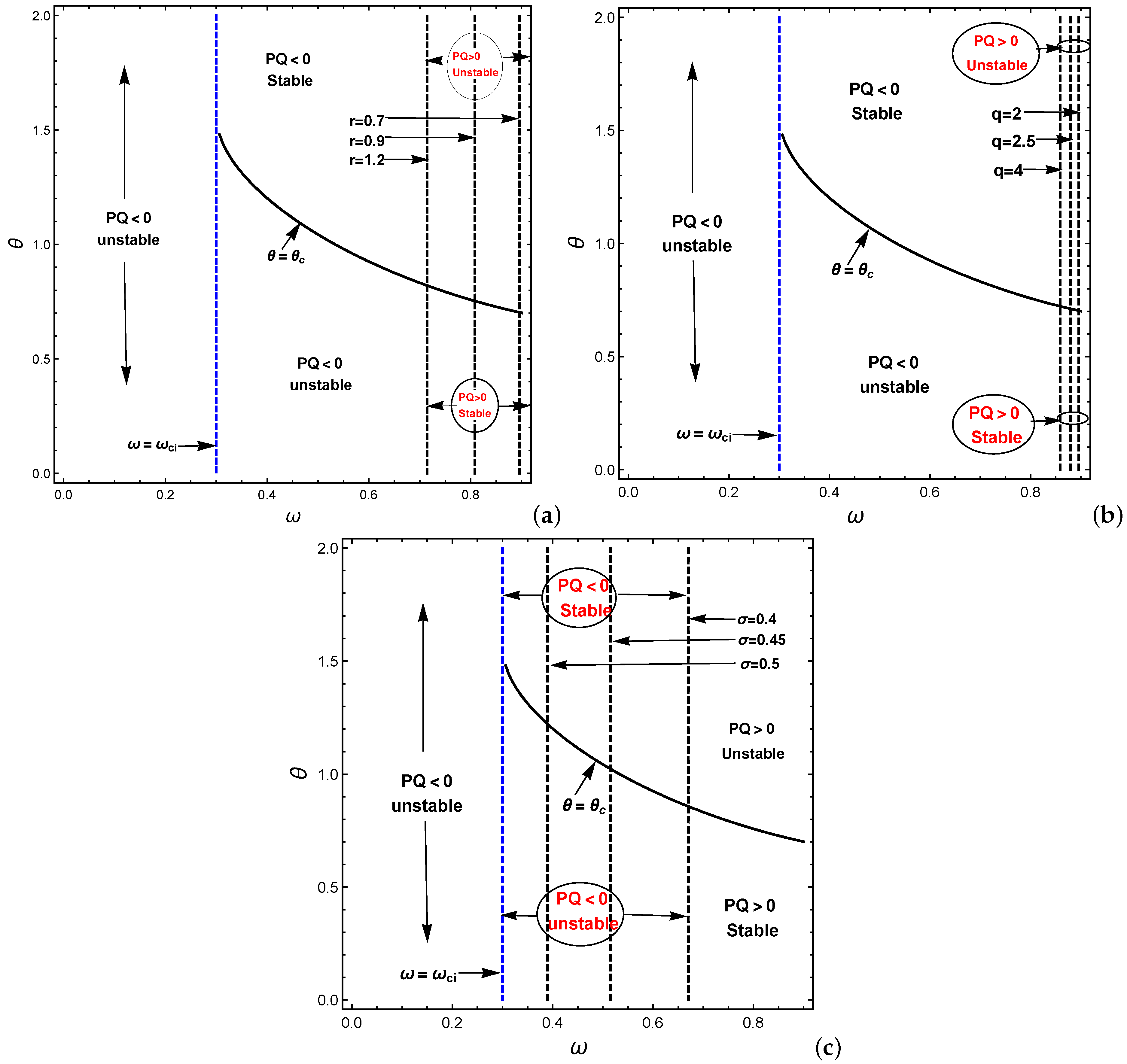
Firstly, our interest is to discuss the effect of the $(r,q)$ distribution parameters and $\sigma =(T_p/T_e)$ on the stability and instability domains for $(H^{+},H^{-})$ electronegative plasma ($\gamma =1$). This is shown in Figure 1. These figures show the $\omega -\theta$ plane for different values of $r,q$, and $\sigma$ at ${\omega }_{ci}=0.3$, which is divided into various stable and unstable regions by the lines $\omega ={\omega }_{ci}$, $\omega ={\omega }_c$, and $\theta ={\theta }_c$. We notice that when $\omega <{\omega }_{ci}$, the product $PQ<0$, the modulational profile of IAWs is independent of the modulational obliqueness $\theta$, and therefore, the IAW is unstable. In contrast, when $\omega ={\omega }_c$, two regions are obtained, i.e., $PQ<0$ (${\omega }_{ci}<\omega <{\omega }_c$) and $PQ>0$ ($\omega >{\omega }_c$), and in these regions, the modulational profile of IAWs is dependent on $\theta$. For $\theta >{\theta }_c$, we have two regions: stable (unstable) corresponding to $PQ<0$ ($PQ>0$). On the contrary, for $\theta <{\theta }_c$, $PQ<0$ (>0) represents an unstable (stable) region, respectively. It is important to mention here that the critical value of the carrier wave frequency ${\omega }_c$ shifts towards lower values by obvious increment change of r, as shown in Figure 1a, but as the spectral index q increases, ${\omega }_c$ decreases slowly, as shown in Figure 1b. Furthermore, the carrier wave frequency ${\omega }_c$ decreases by obvious change as the temperature ratio $\sigma$ increases. We notice from these figures that we obtain one value of the critical ion cyclotron ${\omega }_c$ frequency for each change in the physical parameters of the system. When $\theta >{\theta }_c$, the system is similar to the one-dimensional MI, which has two regions—stable for $PQ<0$ and unstable for $(PQ>0)$. From these regions, we find that the instability of the system increases, and more energy is gained with increasing the effect of highly energetic particles ($(r,q)$ distributed electrons), as well as the positrons temperatures $T_p$ though $\sigma$. In contrast, for $\theta <{\theta }_c$, the stability domain of the system increases as the stable region $(PQ>0)$ increases, and the unstable region $(PQ<0)$ decreases. We find that the study of the waves in 3D gives us a wider range to study the properties of the nonlinear waves in order to understand their features.

Now, let us investigate the role of the other physical parameters of the system on the propagation of the IARWs properties for our plasma system. The first-order RW solution is given as [52,55]

$$\Phi =\sqrt{\frac{2R+P}{Q}}\times \left[\frac{-3+2{(\zeta +\eta +\chi )}^2+4{\tau }^2{(2R+P)}^2-8i\tau (2R+P)}{1+2{(\zeta +\eta +\chi )}^2+4{\tau }^2{(2R+P)}^2}\right]exp\left[i\tau (2R+P)\right],$$

(26)

whereas the second-order RW solution is given by [52]

$$\Phi =\sqrt{\frac{2R+P}{Q}}\times \left[1+\frac{E_2+i{F}_2}{G_2}\right]exp\left[i\tau (2R+P)\right],$$

(27)

with $E_2,F_2$, and $G_2$ having the forms

$$E_2=\frac{3}{8}-9{\tau }^2{(2R+P)}^2-\frac{3}{2}{(\zeta +\eta +\chi )}^2-10{\tau }^4{(2R+P)}^4-\frac{1}{2}{(\zeta +\eta +\chi )}^4-6{(\zeta +\eta +\chi )}^2{\tau }^2{(2R+P)}^2,$$

(28)

$$F_2=\tau (2R+P)\left\{\begin{array}{c}-{\displaystyle \frac{15}{4}}+2{\tau }^2{(2R+P)}^2-3{(\zeta +\eta +\chi )}^2+4{\tau }^4{(2R+P)}^4\hfill \\ +4{(\zeta +\eta +\chi )}^2{\tau }^2{(2R+P)}^2+{(\zeta +\eta +\chi )}^4\hfill \end{array}\right\},$$

and

$$\begin{array}{c}{G}_2=\frac{3}{32}+\frac{33}{8}{\tau }^2{(2R+P)}^2+\frac{1}{2}{(\zeta +\eta +\chi )}^4{\tau }^2{(2R+P)}^2+\frac{9}{2}{\tau }^4{(2R+P)}^4-\frac{3}{2}{(\zeta +\eta +\chi )}^2{\tau }^2{(2R+P)}^2\hfill \\ \hfill +\frac{1}{8}{(\zeta +\eta +\chi )}^4+\frac{2}{3}{\tau }^6{(2R+P)}^6+\frac{1}{12}{(\zeta +\eta +\chi )}^6+{(\zeta +\eta +\chi )}^2{\tau }^4{(2R+P)}^4+\frac{9}{16}{(\zeta +\eta +\chi )}^2.\end{array}$$

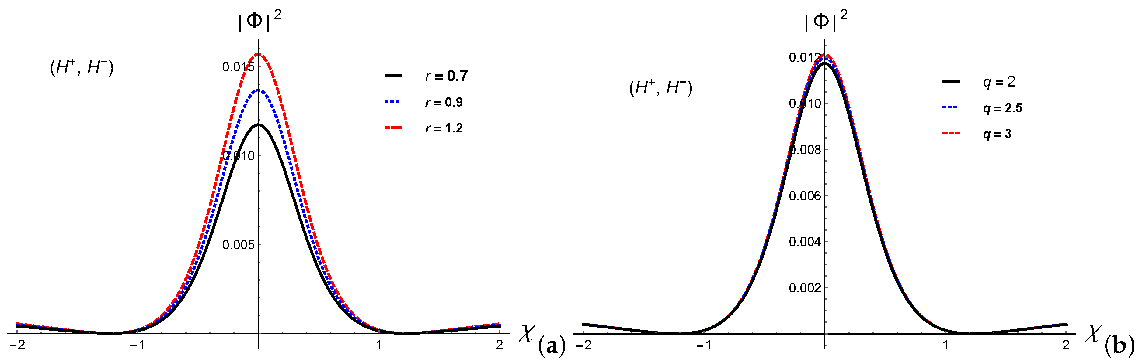
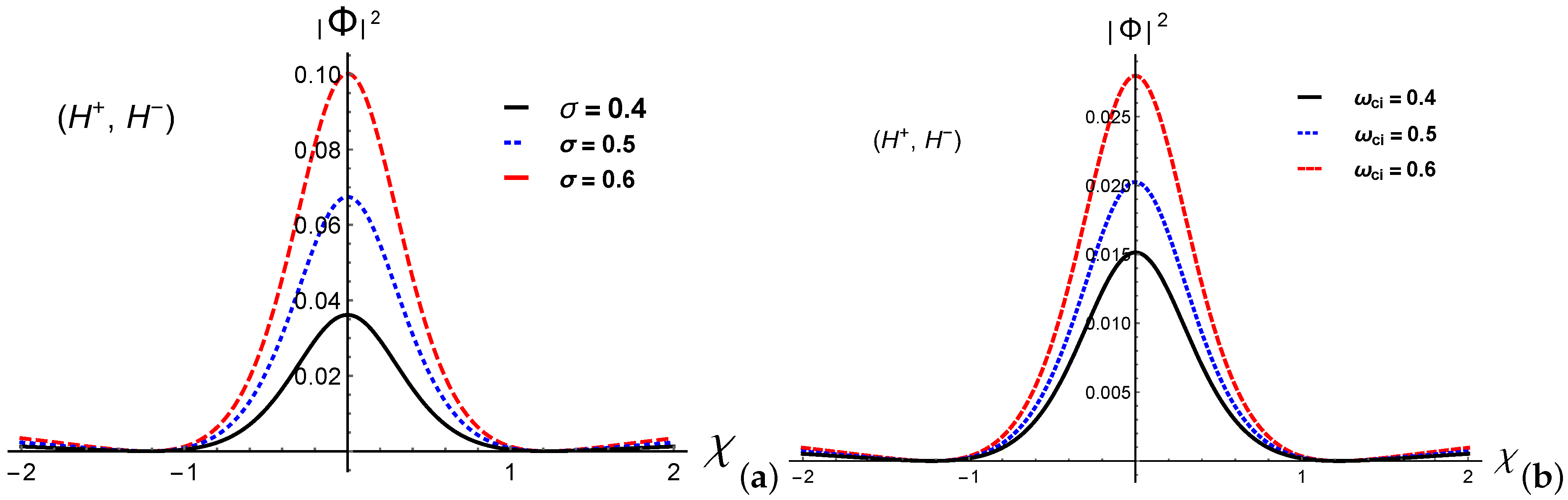
Figure 2 and Figure 3 show the dependence of the nonlinear first-order IARWs formed in the $(H^{+},H^{-})$ electronegative plasma media. We notice here that the profiles of IAWs solution introduced in Equation (25) are significantly modified by the above-mentioned parameters. Figure 2 shows that the width and the amplitude of the first-order IARWs for $(H^{+},H^{-})$ electronegative plasma increase by increasing the effect of non-Maxwellian particles through the increase of r and q. This means that the non-Maxwellian particles improve the nonlinearity of the system, in which the RWs accumulate more to passing through the ionospheric ions of Earth’s ionosphere. Furthermore, increasing the temperature ratio $\left(\sigma \right)$ and the magnetic field through ${\omega }_{ci}$ enhances the width and the amplitude of IARWs. According to these increases in energy, the RWs may be a tool to transfer the energy from/to ionospheric ions or may be a catalyst for chemical reactions in Earth’s ionosphere. The effects obtained for $(H^{+},H^{-})$ electronegative plasma cases can also be obtained for $(H^{+},O_2^{-})$ plasma by a proper choice of the physical parameters of the electronegative plasma systems. However, we do not provide them here.

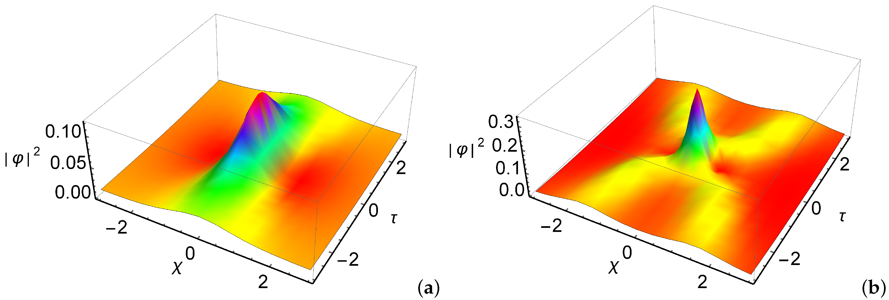
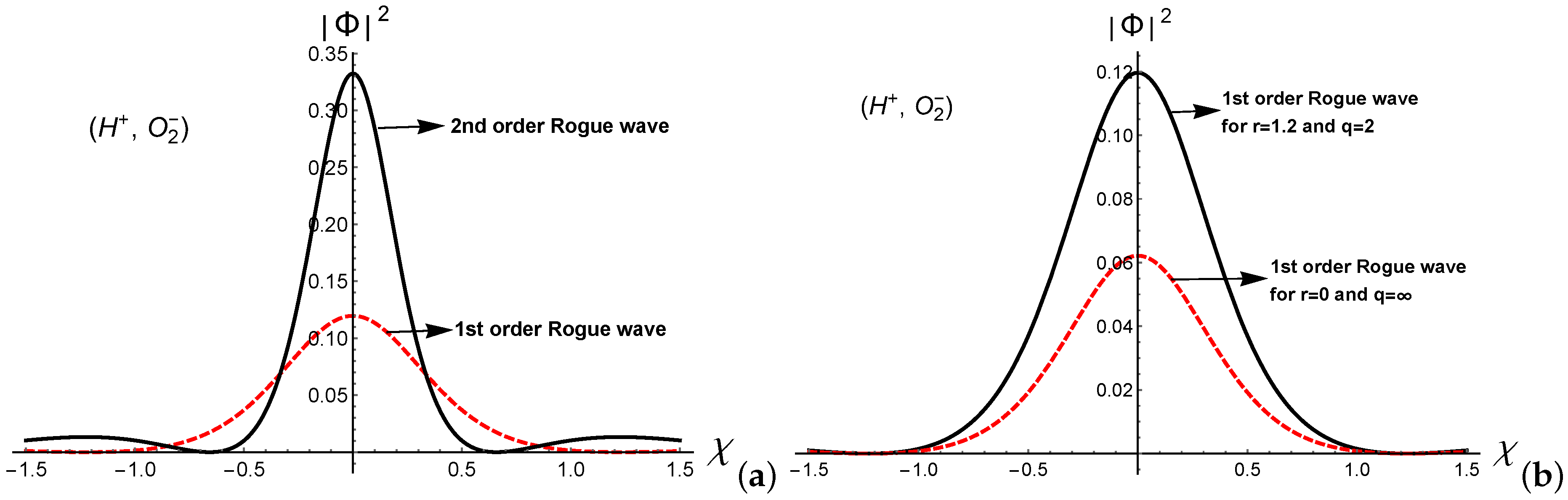
Figure 4 shows the 3D plot of the amplitudes of the first- and second-order IARWs, respectively, formed in the $(H^{+},H^{-})$ electronegative plasma system. Furthermore, Figure 5a illustrates a comparison between the amplitudes of the first-and second-order IARWs for $(H^{+},O_2^{-})$ plasma. We can recognize that the amplitude of the second-order IARWs is narrower, and it is about three times of the first-order IARWs [52,56]. This means that the second-order IARWs accumulate extra energy from the background waves, and more energy is concentrated in narrow regions rather than the first-order IARWs. It is clear that the second-order IARWs involve much more complicated nonlinear profiles. In addition, Figure 5b displays a comparison between the amplitude of the first-order IARWs obtained by $(r,q)$ distribution and the case corresponding to $r=0$, $q⟶\infty$ [where $(r,q)$ distributed electrons and positrons proceed to Maxwellian ones]. It is clear from this figure that the amplitude of first-order IARWs obtained by $(r,q)$ distribution is wider and has higher nonlinearity than that obtained for the Maxwellian case. This means that the Maxwell distribution is not suitable for describing the highly energetic particles, and the non-Maxwellian $(r,q)$ distribution is more adequate.

4. Conclusions

In the present work, the MI as well as the nonlinear properties of IARWs for $(H^{+},H^{-})$ and $(H^{+},O_2^{-})$ electronegative plasmas in a four-component magnetized plasma system, which consists of positive and negative ions fluids, non-Maxwellian $(r,q)$ distributed species for both electrons and positrons are investigated.

The main results of this research can be summarized as follows:

1. The basic system of equations is reduced to a 3D NLSE using the derivative expansion method.

2. The domains of the stability and instability are found to be dependent on the modulational obliqueness $\theta$ and are also strongly affected by the generalized $(r,q)$ distribution parameters as well as the temperature ratio $\sigma [=T_p/T_e]$.

3. The existence domains for the first-and second-order solutions of IARWs are determined and numerically analyzed.

4. The width and the amplitude of the first-order IARWs are modified by increasing the generalized $(r,q)$ distribution parameters, positive ion cyclotron frequency $\left({\omega }_{ci}\right)$ and positron-to-electron temperature ratio $\sigma$. The IARWs gain more energy where the nonlinearity of the system is enhanced by increasing plasma system parameters.

5. The width and amplitude of the second-order IARWs are narrower and higher than the amplitude of the first- order IARWs. This means that the second-order solution has extra poles which accumulate extra energy on the onset of the instability.

6. The amplitude and the width of the first-order IARWs obtained by $(r,q)$ distribution are higher and wider than those of the Maxwellian one.

A good agreement is found between our work for $r=0$ and $q⟶\infty$ with that obtained by Haque and Mannan [18] when the nonthermal parameter $\beta =0$ in their work. Our results of the present work are useful for interpreting the MI of IAW and the formation propagation properties of IARW amplitude in D–F regions of Earth’s ionosphere through $(H^{+},O_2^{-})$ and $(H^{+},H^{-})$ electronegative plasma [5,9].

References

- Kelly, M. The Earth’s Ionosphere: Plasma Physics and Electrodynamics; Elsevier: Amsterdam, The Netherlands, 2012; Volume 43. [Google Scholar]
- Grandian, M. Multi-Instrument and Modelling Studies of Ionospheres at Earth and Mars. Ph.D. Thesis, Université Toulouse 3 Paul Sabatier (UT3 Paul Sabatier), Toulouse, France, November 2017. [Google Scholar]
- El-Labany, S.; Sabry, R.; El-Taibany, W.; Elghmaz, E. Propagation of three-dimensional ion-acoustic solitary waves in magnetized negative ion plasmas with nonthermal electrons. Phys. Plasmas 2010, 17, 042301. [Google Scholar] [CrossRef]
- Chowdhury, N.; Mannan, A.; Hasan, M.; Mamun, A. Heavy ion-acoustic rogue waves in electron-positron multi-ion plasmas. Chaos 2017, 27, 093105. [Google Scholar] [CrossRef]
- Abdelwahed, H.; Sabry, R.; El-Rahman, A. On the positron superthermality and ionic masses contributions on the wave behaviour in collisional space plasma. Adv. Space Res. 2020, 66, 259. [Google Scholar] [CrossRef]
- Bacal, M.; Hamilton, G. H− and D− Production in Plasmas. Phys. Rev. Lett. 1979, 42, 1538. [Google Scholar] [CrossRef]
- Gottscho, R.A.; Gaebe, C.E. Negative Ion Kinetics in RF Glow Discharges. IEEE Trans. Plasma Sci. 1986, 14, 92. [Google Scholar] [CrossRef]
- Pedersen, A. Measurements of ion concentrations in the D-region of the ionosphere with a Gerdien condenser rocket probe. Tellus 1965, 17, 2. [Google Scholar] [CrossRef] [Green Version]
- Sabry, R.; Moslem, W.; Shukla, P.K. Fully nonlinear ion-acoustic solitary waves in a plasma with positive-negative ions and nonthermal electrons. Phys. Plasmas 2009, 16, 032302. [Google Scholar] [CrossRef]
- Chaizy, P.; Reme, H.; Sauvaud, J.; d’Uston, C.; Lin, R.; Larson, D.; Mitchell, D.; Anderson, K.; Carlson, C.; Korth, A.; et al. Negative ions in the coma of comet Halley. Nature 1991, 349, 393. [Google Scholar] [CrossRef]
- Coates, A.; Crary, F.; Lewis, G.; Young, D.; Waite, J.; Sittler, E. Discovery of heavy negative ions in Titan’s ionosphere. Geophys. Res. Lett. 2007, 34. [Google Scholar] [CrossRef] [Green Version]
- Temerin, M.; Cerny, K.; Lotko, W.; Mozer, F. Observations of Double Layers and Solitary Waves in the Auroral Plasma. Phys. Rev. Lett. 1982, 48, 1175. [Google Scholar] [CrossRef]
- Michel, F.C. Theory of Neutron Star Magnetospheres; University of Chicago Press: Chicago, IL, USA, 1991. [Google Scholar]
- Panwar, A.; Ryu, C.; Bains, A. Oblique ion-acoustic cnoidal waves in two temperature superthermal electrons magnetized plasma. Phys. Plasmas 2014, 21, 122105. [Google Scholar] [CrossRef] [Green Version]
- Chowdhury, N.; Mannan, A.; Hasan, M.; Mamun, A. Modulational instability, ion-acoustic envelope solitons, and rogue waves in four-component plasmas. Plasma Phys. Rep. 2019, 45, 459. [Google Scholar] [CrossRef]
- Michel, F.C. Theory of pulsar magnetospheres. Rev. Mod. Phys. 1982, 54. [Google Scholar] [CrossRef]
- Haque, M.; Mannan, A.; Mamun, A. The (3 + 1)-dimensional dust-acoustic waves in multi-components magneto-plasmas. Contrib. Plasma Phys. 2019, 59, e201900049. [Google Scholar] [CrossRef]
- Haque, M.N.; Mannan, A. Dynamics of ion-acoustic rogue waves in electron-positron-ion magneto-plasmas. Contrib. Plasma Phys. 2020, 61, e202000161. [Google Scholar]
- Marklund, M.; Shukla, P.K. Nonlinear collective effects in photon-photon and photon-plasma interactions. Rev. Mod. Phys. 2006, 78, 591. [Google Scholar] [CrossRef] [Green Version]
- Shukla, P.; Yu, M.; Tsintsadze, N. Intense solitary laser pulse propagation in a plasma. Phys. Fluids 1984, 27, 327. [Google Scholar] [CrossRef]
- Shukla, P.; Rao, N.; Yu, M.; Tsintsadze, N. Relativistic nonlinear effects in plasmas. Phys. Rep. 1986, 138, 1. [Google Scholar] [CrossRef]
- Surko, C.; Murphy, T. Use of the positron as a plasma particle. Phys. Fluids B: Plasma Phys. 1990, 2, 1372. [Google Scholar] [CrossRef]
- Sabry, R.; Moslem, W.; Shukla, P.K.; Saleem, H. Cylindrical and spherical ion-acoustic envelope solitons in multicomponent plasmas with positrons. Phys. Rev. E 2009, 79, 056402. [Google Scholar] [CrossRef] [PubMed]
- Shalini, S.; Misra, A. Modulation of ion-acoustic waves in a nonextensive plasma with two-temperature electrons. Phys. Plasmas 2015, 22, 092124. [Google Scholar] [CrossRef] [Green Version]
- Sultana, S.; Kourakis, I. Electrostatic solitary waves in the presence of excess superthermal electrons: Modulational instability and envelope soliton modes. Plasma Phys. Control. Fusion 2011, 53, 045003. [Google Scholar] [CrossRef] [Green Version]
- Baluku, T.; Hellberg, M. Ion acoustic solitons in a plasma with two-temperature kappa-distributed electrons. Phys. Plasmas 2012, 19, 012106. [Google Scholar] [CrossRef]
- Bains, A.; Tribeche, M.; Gill, T. Modulational instability of ion-acoustic waves in a plasma with aq-nonextensive electron velocity distribution. Phys. Plasmas 2011, 18, 022108. [Google Scholar] [CrossRef]
- Sabry, R.; Moslem, W.; Shukla, P. Three-dimensional ion-acoustic wave packet in magnetoplasmas with superthermal electrons. Plasma Phys. Control. Fusion 2012, 54, 035010. [Google Scholar] [CrossRef]
- El-Tantawy, S.; Wazwaz, A.; Rahman, A.U. Three-dimensional modulational instability of the electrostatic waves in e–p–i magnetoplasmas having superthermal particles. Phys. Plasmas 2017, 24, 022126. [Google Scholar] [CrossRef]
- El-Labany, S.K.; El-Taibany, W.F.; El-Bedwehy, N.A.; El-Shafeay, N.A. Modulation of the nonlinear ion acoustic waves in a weakly relativistic warm plasma with superthermally distributed electrons. Alfarama J. Basic Appl. Sci. 2020, 1, 99. [Google Scholar]
- Janssen, P.A. Nonlinear four-wave interactions and freak waves. J. Phys. Oceanogr. 2003, 33, 863. [Google Scholar] [CrossRef]
- Ganshin, A.; Efimov, V.; Kolmakov, G.; Mezhov-Deglin, L.; Clintock, P.V.M. Observation of an inverse energy cascade in developed acoustic turbulence in superfluid helium. Phys. Rev. Lett. 2008, 101, 065303. [Google Scholar] [CrossRef] [Green Version]
- Shats, M.; Punzmann, H.; Xia, H. Capillary Rogue Waves. Phys. Rev. Lett. 2010, 104, 104503. [Google Scholar] [CrossRef]
- Bludov, Y.V.; Konotop, V.; Akhmediev, N. Matter rogue waves. Phys. Rev. A 2009, 80, 033610. [Google Scholar] [CrossRef] [Green Version]
- Sabry, R.; Moslem, W.; Shukla, P. Freak waves in white dwarfs and magnetars. Phys. Plasmas 2012, 19, 122903. [Google Scholar] [CrossRef]
- Abdelwahed, H.; El-Shewy, E.; Zahran, M.; Elwakil, S. On the rogue wave propagation in ion pair superthermal plasma. Phys. Plasmas 2016, 23, 022102. [Google Scholar] [CrossRef]
- Ahmed, N.; Mannan, A.; Chowdhury, N.A.; Mamun, A.A. Electrostatic rogue waves in double pair plasmas. Chaos 2018, 28, 123107. [Google Scholar] [CrossRef] [Green Version]
- Hassan, M.; Rahman, M.H.; Chowdhury, N.A.; Mannan, A.; Mamun, A.A. Ion-acoustic rogue waves in multi-ion plasmas. Commun. Theor. Phys. 2019, 71, 1017. [Google Scholar] [CrossRef] [Green Version]
- Khondaker, S.; Mannan, A.; Chowdhury, N.A.; Mamun, A.A. Rogue waves in multi-pair plasma medium. Contrib. Plasma Phys. 2019, 59, e201800125. [Google Scholar] [CrossRef] [Green Version]
- Jahan, S.; Haque, M.N.; Chowdhury, N.A.; Mannan, A.; Mamun, A.A. Ion-acoustic rogue waves in double pair plasma having non-extensive particles. Universe 2021, 7, 63. [Google Scholar] [CrossRef]
- Rahman, M.H.; Chowdhury, N.A.; Mannan, A.; Rahman, M.; Mamun, A.A. Modulational instability, rogue waves, and envelope solitons in opposite polarity dusty plasmas. Chin. J. Phys. 2018, 56, 2061. [Google Scholar] [CrossRef] [Green Version]
- Chowdhury, N.A.; Mannan, A.; Mamun, A.A. Rogue waves in space dusty plasmas. Phys. Plasmas 2017, 24, 113701. [Google Scholar] [CrossRef]
- Rajib, T.I.; Tamanna, N.K.; Chowdhury, N.A.; Mannan, A.; Sultana, S.; Mamun, A.A. Dust-ion-acoustic rogue waves in presence of non-extensive non-thermal electrons. Phys. Plasmas 2019, 26, 123701. [Google Scholar] [CrossRef]
- Jahan, S.; Mannan, A.; Chowdhury, N.A. Dust-acoustic rogue waves in four-component plasmas. Plasma Phys. Rep. 2020, 46, 90. [Google Scholar] [CrossRef] [Green Version]
- Rahman, M.; Chowdhury, N.A.; Mannan, A.; Mamun, A.A. Dust-acoustic rogue waves in an electron-positron-ion-dust plasma medium. Galaxies 2021, 9, 31. [Google Scholar] [CrossRef]
- Sikta, J.N.; Chowdhury, N.A.; Mannan, A.; Sharmin, S.; Mamun, A.A. Electrostatic Dust-Acoustic Rogue Waves in an Electron Depleted Dusty Plasma. Plasma 2021, 4, 15. [Google Scholar] [CrossRef]
- Vasyliunas, V.M. A survey of low-energy electrons in the evening sector of the magnetosphere with OGO 1 and OGO 3. J. Geophys. Res. 1968, 73, 2839. [Google Scholar] [CrossRef]
- Zaheer, S.; Murtaza, G.; Shah, H. Some electrostatic modes based on non-Maxwellian distribution functions. Phys. Plasmas 2004, 11, 2246. [Google Scholar] [CrossRef]
- Qureshi, M.; Shah, H.; Murtaza, G.; Schwartz, S.; Mahmood, F. Parallel propagating electromagnetic modes with the generalized (r, q) distribution function. Phys. Plasmas 2004, 11, 3819. [Google Scholar] [CrossRef]
- El-Taibany, W.; Taha, R. Variable-size dust grains with generalized (r, q) electrons in a dusty plasma. Contrib. Plasma Phys. 2019, 59, e201800072. [Google Scholar] [CrossRef]
- El-Bedwehy, N.; El-Taibany, W.F. Modulational instability of dust-ion acoustic waves in the presence of generalized (r, q) distributed electrons. Phys. Plasmas 2020, 27, 012107. [Google Scholar] [CrossRef]
- Guo, S.; Mei, L. Three-dimensional dust-ion-acoustic rogue waves in a magnetized dusty pair-ion plasma with nonthermal nonextensive electrons and opposite polarity dust grains. Phys. Plasmas 2014, 21, 082303. [Google Scholar] [CrossRef]
- Yahia, M.E.; Tolba, R.E.; Moslem, W.M. Super rogue wave catalysis in Titan’s ionosphere. Adv. Space Res. 2021, 67, 1412. [Google Scholar] [CrossRef]
- Peregrine, D.H. Water waves, nonlinear Schrödinger equations and their solutions. Anziam J. 1983, 25, 16. [Google Scholar] [CrossRef] [Green Version]
- Akhmediev, N.; Ankiewicz, A.; Soto-Crespo, J.M. Rogue waves and rational solutions of the nonlinear Schrödinger equation. Phys. Rev. E 2009, 80, 026601. [Google Scholar] [CrossRef] [PubMed] [Green Version]
- Abdelwahed, H.; Sabry, R. Modulated 3D electron-acoustic rogue waves in magnetized plasma with nonthermal electrons. Astrophys. Space Sci. 2017, 362, 92. [Google Scholar] [CrossRef]
Figure 1.
Plot of the product versus and for different values of r with (a), q with and (b), and with and (c). Here, , , and .
Figure 2.
The change of first-order IARWs amplitude versus for various values of r with (a) and q with (b). Here, , , , and .
Figure 3.
The change of first-order IARWs amplitude versus for various values of with . (a) and with (b). Here, , , , and .
Figure 4.
The 3D plot of the amplitude of the first-order (a) and second-order (b) IARWs for electronegative plasma (where and ). Here , , , , , and .
Figure 5.
The amplitude of the first-and second-order IARWs with and (a) and the first-order IARWs amplitude obtained by non-Maxwellian and Maxwellian distributed for both electrons and positrons () (b) versus (where and are equal to zero) for electronegative plasma. Here , , , and .
Publisher’s Note: MDPI stays neutral with regard to jurisdictional claims in published maps and institutional affiliations. |
© 2021 by the authors. Licensee MDPI, Basel, Switzerland. This article is an open access article distributed under the terms and conditions of the Creative Commons Attribution (CC BY) license (https://creativecommons.org/licenses/by/4.0/).
Share and Cite
MDPI and ACS Style
El-Taibany, W.F.; El-Bedwehy, N.A.; El-Shafeay, N.A.; El-Labany, S.K. Three-Dimensional Rogue Waves in Earth’s Ionosphere. Galaxies 2021, 9, 48. https://0-doi-org.brum.beds.ac.uk/10.3390/galaxies9030048
AMA Style
El-Taibany WF, El-Bedwehy NA, El-Shafeay NA, El-Labany SK. Three-Dimensional Rogue Waves in Earth’s Ionosphere. Galaxies. 2021; 9(3):48. https://0-doi-org.brum.beds.ac.uk/10.3390/galaxies9030048
Chicago/Turabian StyleEl-Taibany, Wael F., Nabila A. El-Bedwehy, Nora A. El-Shafeay, and Salah K. El-Labany. 2021. "Three-Dimensional Rogue Waves in Earth’s Ionosphere" Galaxies 9, no. 3: 48. https://0-doi-org.brum.beds.ac.uk/10.3390/galaxies9030048
Note that from the first issue of 2016, this journal uses article numbers instead of page numbers. See further details here.