Application of Spatio-Temporal Spectral Analysis for Detection of Seismic Waves in Gravitational-Wave Interferometer

Abstract

Mixed spatio–temporal spectral analysis was applied for the detection of seismic waves passing through the west–end building of the Virgo interferometer. The method enables detection of a passing wave, including its frequency, length, direction, and amplitude. A thorough analysis aimed at improving sensitivity of the Virgo detector was made for the data gathered by 38 seismic sensors, in the two–week measurement period, from 24 January to 6 February 2018, and for frequency range 5–20 Hz. Two dominant seismic–wave frequencies were found: 5.5 Hz and 17.1 Hz. The presented method can be applied for a better understanding of the interferometer seismic environment, and by identifying noise sources, help the noise–hunting and mitigation work that eventually leads to interferometer noise suppression.

1. Introduction

The first events detected by gravitational–wave (GW) detectors in the past decade have given us hope to answer the most fundamental questions of astronomy and physics, concerning, e.g., evolution of galaxies and black holes, gravitational collapse of supernovae, and limits of general relativity [1,2,3,4,5,6]. However, noise reduction in these detectors is a most complex task, due to very low amplitude of the incoming signals. Seismic characterization of the vicinity of the GW detectors is necessary for the noise reduction. The method presented in this paper enables the identification of such signals. This characterization can help noise mitigation, especially for Newtonian noise coming from fluctuating gravitational forces caused by density perturbations of the ground and of the atmosphere [7,8,9,10]. The data for this paper are seismic data of Newtonian noise array of the seismic sensors installed at west–end building (WEB) of the Virgo GW detector [11]. Virgo arms named West and North are orientated approx. 20${}^{°}$ clockwise from North. The Virgo coordinate system is centered on the beam splitter in the central building.

Spatio–temporal spectral analysis is a straightforward extension of harmonic analysis to more than one dimension. Apart from a temporal dimension, additional spatial dimensions are introduced. The method allows identification of the frequencies and the wave vectors of waves passing through the Virgo detector. The input data for our analysis contains spatial and temporal dimensions. Spatial part should have fixed boundaries. In such cases we can look for modes of variability, i.e., underlying spatio–temporal structures with preferred spatial pattern and temporal variation. If the signal is harmonic (wavelike), then we expect spatio–temporal spectral analysis to isolate any such modes that are present in the data. For instance, if we make spatio–temporal spectral analysis of a string instrument, we expect to find a definite relationship between the length scales and the time scales of the oscillations [12].

The method presented in this article is based on paper [13] and refs. therein, where seismic–noise structure has been estimated using arrays of detectors (see also [14]). Spatio–temporal spectral analysis has been used before to obtain the Rayleigh wave phase velocity dispersion curves [15]. It is also a widely explored method in the atmospheric sciences [16,17,18,19,20]. Moreover, [21] applied spatio–temporal spectral analysis to modeling rainfall fields. As far as only spatial Fourier transform is concerned, Kim and Barros [22] used its two–dimensional version to analyze the structure of soil moisture fields in different time moments, considered separately.

Investigations of the seismic characteristics of the Virgo site have been made previously in [23,24,25]. For recent works about seismic–noise measurements for gravitational–wave detectors see, e.g., [26,27,28,29].

This paper is structured as follows. The system of seismometers that we used for data acquisition is presented in Section 2. Then, we provide information about data analysis process in Section 3. The results of this analysis are described in Section 4. Finally, concluding remarks are given in Section 5.

2. Measuring System

For this study, a system of seismic sensors in the west–end building (WEB) of the Virgo interferometer was examined. The system consists of 38 Innoseis Tremornet seismometers [30], deployed on the building floor. The exact coordinates of the seismometers are provided in Appendix A. The average distance between the seismometers was approximately 9.5 m. Point $(0,0)$ of the coordinate system is the interferometer beam splitter mirror. The axes coincide with the Virgo arms.

The floor is supported by 30 m long poles, while the central platform and the basement are supported by a set of longer poles reaching a more stable gravel layer, at 52 m depth. Seismometers no. 1–23 were placed on the floor of the building, no. 24–38—on the central platform, while no. 37 and 38—in the basement. Vacuum chamber rests on the central platform at WEB (and north–end building as well) where one of the four mirror test masses of Virgo is located and suspended to a vibration isolation system. The construction also provides suppression of seismic noise above 15 Hz on the central platform. For frequency values above ca. 15 Hz, there is a significant difference in the amplitude spectral densities (ASDs) between the platform and the floor [29].

The sensors were placed on the floor fixing their mount plate with double–sided adhesive tape for a good connection to ground. The sensors are 4.5 Hz geophones and have a flat response function in the range from 4.5 to at least 50 Hz where we present this analysis. Each sensor measure, the vertical ground velocity [30] and also contains a preamplifier and a 24–bit analog to digital converter. The digital signal of each sensor is transferred to a centralized unit through ethernet cable and then stored. The seismometers measure voltage changes in the range between $-5$ V and 5 V with sensitivity (manufacturer defined) 77.3 V/m/s. Seismometer signals were converted from volts to m/s, by using the appropriate conversion coefficient $5/(2^{23}\times 77.3)$. For more details see [31].

The data that were used for the calculations were collected during a two–week measurement period, from 24 January to 6 February 2018. The data of each sensor are recorded with 500 Hz sampling frequency. Not all the 256 1-h data files generated in the measurement period are complete. The effective measurement time is 250 h (∼10.5 days). A series of 10 consecutive zeros was assumed being empty–data period for this sensor. Empty periods amount to $3.4\%$ of the total data.

3. Methodology

We indicate with $\psi (x,y,t)$ the vertical velocity measured at time t of the seismometer positioned at coordinates $(x,y)$. We apply the mixed spatio–temporal Fourier transform (FT) to obtain the quantity $\mathrm{FT}(k_x,k_y,\omega )$, where $k_x,k_y$ are the components of the wave–vector $\overrightarrow{\mathbf{k}}=\frac{2\pi }{\lambda }\widehat{\mathbf{r}}$, where $\lambda$ is the wavelength, and $\omega$ is the wave frequency. The spatio–temporal transform is defined as:

$$\mathrm{FT}(k_x,k_y,\omega )=\int dt\int dx\int dy\psi (x,y,t)e^{-i(\omega t+k_{x}x+k_{y}y)}$$

(1)

Time t is discretized with $\Delta t=0.002$ s. The value of $\mathrm{FT}(k_x,k_y,\omega )$ provides information about the amplitude of the particular wave.

In general, the spatio–temporal Fourier transform consists of wave vectors for each wave detected in the signal (represented along the $k_x,k_y$ axes) together with the frequency of that wave (on $\omega$ axis). Therefore, we can obtain length, direction, frequency and amplitude (The wave amplitude can be obtained by calculating an inverse Fourier transform of each ASD peak in the final result. However, we must consider in this case all rescalings done during the process of the FT calculation—see below in this section.) of a wave that passed through the measuring system during the considered time period. Notably, Rayleigh surface waves are expected to prevail in the seismic wavefield in the vicinity of the Virgo west–end building [32]. Therefore, we can neglect vertical differences between the spatial positions of the seismometers (z axis).

Remarkably, spatio–temporal Fourier transform, as any other multi–dimensional Fourier transform, can be computed in two steps. Having the input data of $(x,y,t)$–points, we can calculate, first, only the temporal part [obtaining $(x,y,\omega )$–points] and subsequently we can calculate the spatial part, obtaining as final result the $(k_x,k_y,\omega )$–points.

In the approach presented herein, at first, the average value of the signal was subtracted from the input, for each sensor separately. Then, the whole signal was divided into 20–s long segments (time frames), 10,000 samples each. By dividing the data into short pieces, we can detect short wave impulses, lasting only a couple of seconds. Due to the fact that the spatio–temporal method, as any other Fourier–based method, uses finite sets of data, the questions of spectral leakage and, consequently, the necessity of applying appropriate windowing functions should be considered to avoid artificial components to appear in the final result. For that purpose the Hann window function was used.

After the initial preparation of data, explained above, the time–frequency part, for every time frame and for each sensor separately, was calculated, using FFT (Fast Fourier Transform) algorithm. After that, the result was multiplied by the appropriate sensor response function, which depends on the frequency value $\omega$. Subsequently, the spatial part was calculated, variables $(x,y)$ were changed to $u=s_{f}x$ and $v=s_{f}y$, where

$$s_f=\frac{\pi }{max\left\{{\left|x\right|}_{max},{\left|y\right|}_{max}\right\}},$$

(2)

so that both spatial dimensions were normalized to $(-\pi ,\pi )$ range. ($(-\pi ,\pi )$ range is needed for NUFFT algorithm—see Section 4).

Finally, the variables were changed back to $k_x=s_f{k}_u$, $k_y=s_f{k}_v$, and three–dimensional complex modulus of the spectrum was calculated to obtain the 3D amplitude spectral density (ASD):

$$\mathrm{ASD}(k_x,k_y,\omega )=\left|\mathrm{FT}(k_x,k_y,\omega )\right|{\left(TXY\right)}^{-1/2},$$

(3)

where $\mathrm{FT}(k_x,k_y,\omega )$ is the spatio–temporal Fourier transform of the measurement data defined in Equation (1), and $T,X,Y$ are the temporal and spatial extent of the data respectively.

3.1. Test Data

To test the algorithm, the following simulation was run. We created a simulated set of data adopting the same $(x,y)$ positions of the seismometers the superposition of two sinusoidal waves:

$$\psi (x,y,t)=Acos(k_{x}x-{\omega }_{1}t)+Bcos(k_{y}y-{\omega }_{2}t),$$

(4)

where $k_x=0.578{\mathrm{m}}^{-1}$, $k_y=-0.876{\mathrm{m}}^{-1}$, ${\omega }_1=3\left(2\pi \right)\mathrm{Hz}$, ${\omega }_2=5\left(2\pi \right)\mathrm{Hz}$, and for instance $A=B=1000$ V. (To mimic the seismometer measurements in volts, approximated to integer values, due to the fact that the real seismometer measurements in volts were integer values. However, before the process of ASD calculation, the units were converted from volts to m/s—cf. Section 3.) The artificial data in volts are converted to m/s.

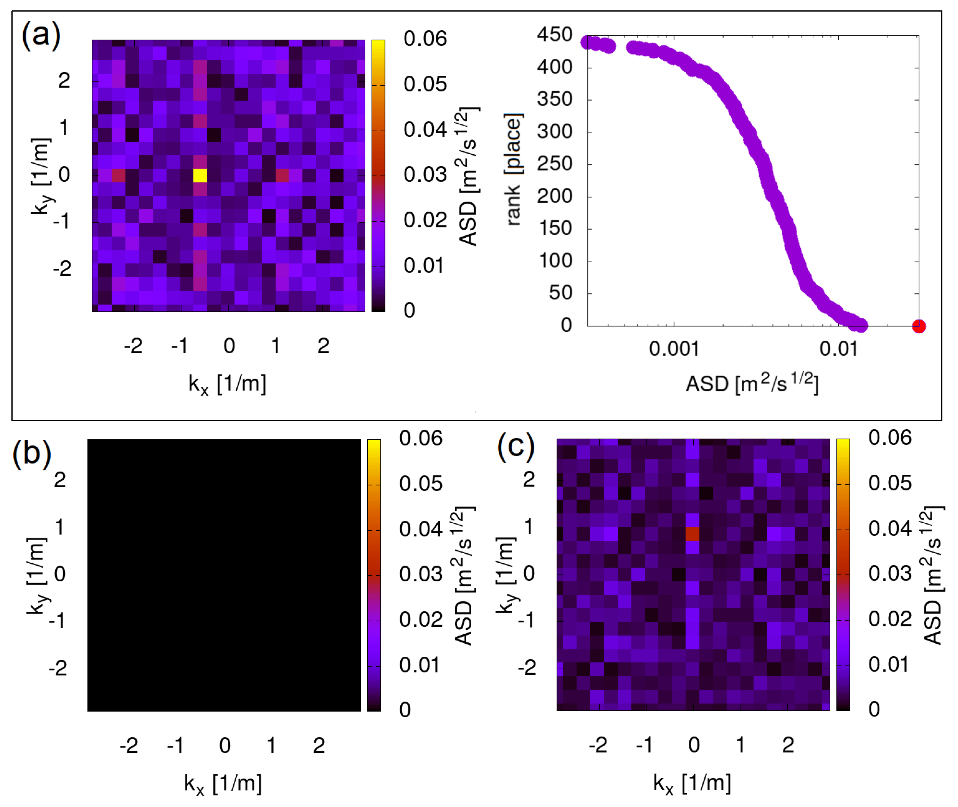
Figure 1 shows the obtained spatio–temporal amplitude spectral density for these exemplary data, in a form of colormap, for 3, 4, and 5 Hz. Additionally, a rank of ASD values is shown for frequency 3 Hz. The right panel of Figure 1a shows the inverse cumulative plot of all the points from the left panel, ordered from the largest to the smallest ASD value. The red dot represents the maximum corresponding to the yellow point in the left panel. This illustrates that the numerical noise due to non–uniform spatial sensor grid is negligible.

As expected, the spatio–temporal amplitude spectral density for such strong signal consists of two outstanding peaks for frequency 3 Hz and 5 Hz (Figure 1a,c), corresponding to both parts of the superpositioned wave, with proper wave–vector and frequency values. Both peaks are outstanding compared to the other spatial modes for frequencies 3 Hz and 5 Hz. The peaks that correspond to 3 Hz and 5 Hz are larger than the average value by about 10 times the standard deviation of the data. We also present the rank plot for the case of 3 Hz, Figure 1a on the right, the outstanding $\mathbf{k}$–value is denoted by the red dot in the bottom right corner, which stands above the remaining data significantly. As expected, no outstanding mode is found at 4 Hz [Figure 1b]. We conclude that the method is robust with respect to identification of the frequency of the waves, but it introduces some noise related to the non–uniform spatial grid.

3.2. Measurement Data

After the successful test of the algorithm on the artificial data, the analysis of the real data collected from the Virgo west–end building was made. In the initial step, the seismometer indications in volts were converted to the appropriate values in m/s (cf. Section 3). Then, the three–dimensional transforms for these data were calculated using FFT and NUFFT algorithms (cf. Section 3). 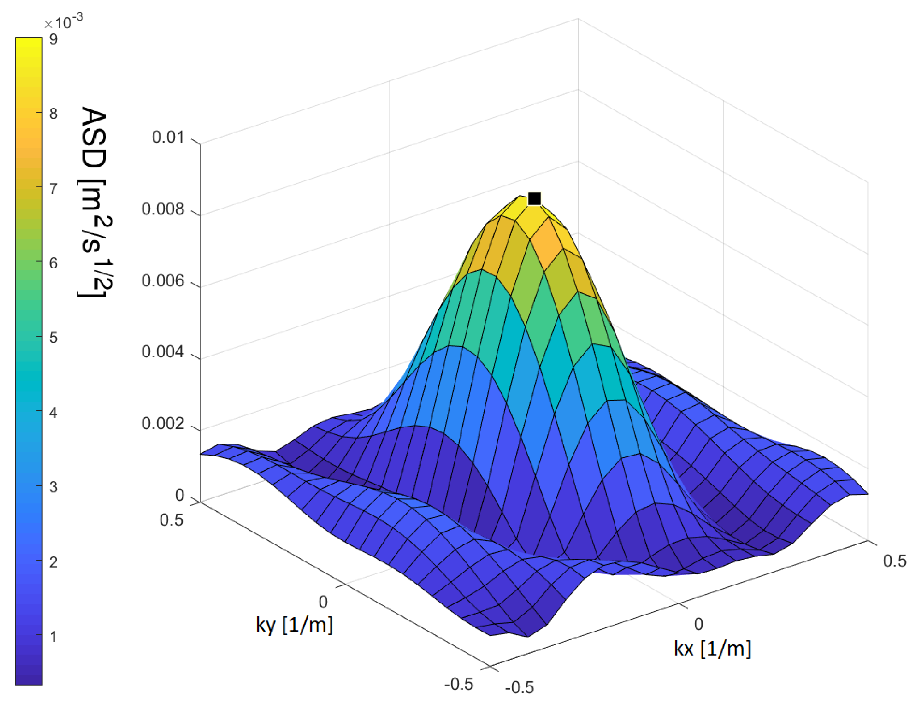The Non–Uniform FFT algorithm (NUFFT) [33,34,35] is the version of FFT algorithm for non–uniform samples, as the locations of the seismometers were not uniform. A version of the NUFFT algorithm for two dimensions was applied. Finally, the spatio–temporal amplitude spectral density was calculated for each 20–s period and each frequency. An example plot is usually characterized by one main maximum—cf. Figure 2.

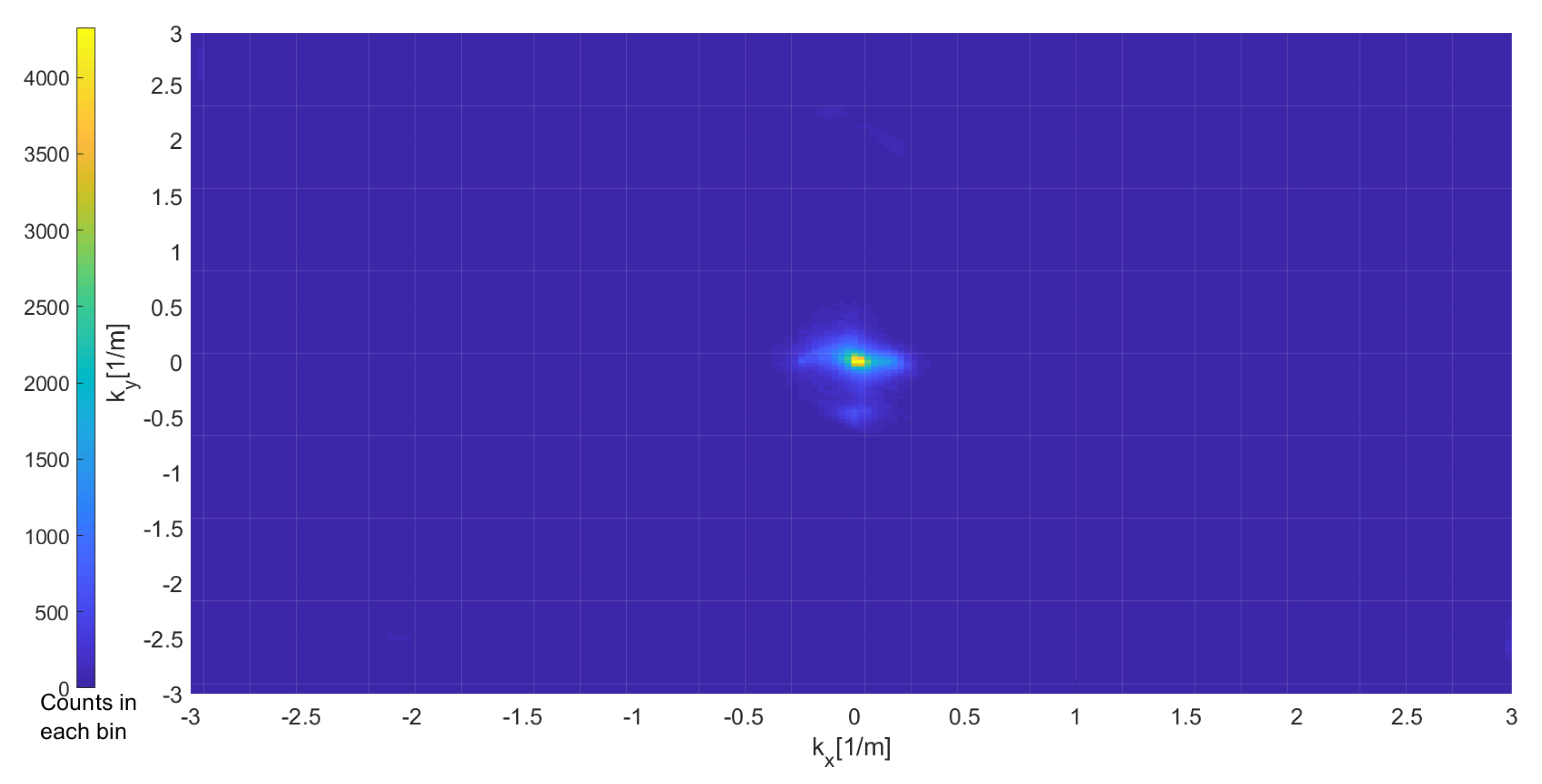
The next step was finding a position $(k_x,k_y)$ of maximal ASD value in time, for each frequency from 5 Hz to 20 Hz, step 0.1 Hz. For the data from a dozen hours of the experiment, a wide range of the wave–vector k was checked. Over 95% of the maximum ASD values found for any frequency in each 20–s period are in the range k from −0.5 to 0.5 1/m (Figure 3). Moreover, the maxima found outside this inner range were very low and likely corresponded to noise. Therefore, we have adopted this smaller range for all calculations.

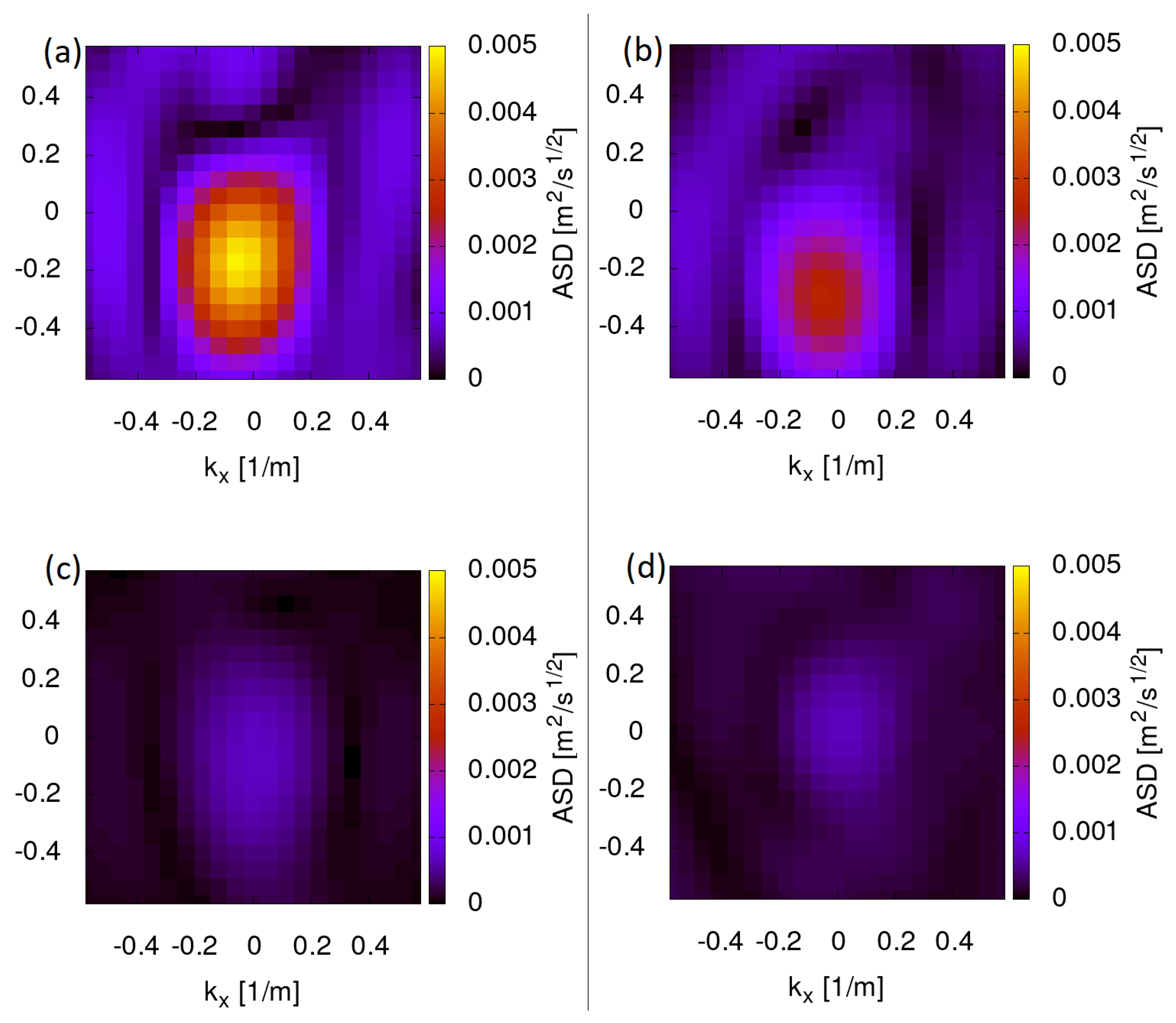
Examples of preliminary results for 20-s pieces of seismic data, taken from the same hour of measurement, are shown in Figure 4.

There are dominant waves for particular frequencies, as expected. In the first plot for 5 Hz [Figure 4a] there is a strong maximum. In Figure 4b for 10 Hz there is much weaker and fuzzy maximum. For Figure 4c,d (12 Hz and 15 Hz, respectively) there are not any signals visible, but rather some artifacts present due to inaccuracy of the measurement or the NUFFT method used.

3.3. Dominant Waves

Resolution of wave–vector space and frequencies taken for our calculation is ${\delta }_k=0.05{\mathrm{m}}^{-1}$, ${\delta }_{\omega }=0.1$ Hz, and we investigated the region of wave–vector space with the size of $-0.5{\mathrm{m}}^{-1}<k_x,k_y<0.5{\mathrm{m}}^{-1}$, thus, for each frequency, there were 180 matrices $21\times 21$ were obtained per hour of data. In order to determine dominant waves the following function (paraboloid, usually looks like our results from Figure 2) was fitted to the spatio–temporal Fourier spectra:

$$\mathrm{f}(u,v)=A-{\frac{u}{{\sigma }_u}}^2-{\frac{v}{{\sigma }_v}}^2,$$

(5)

where A is maximal amplitude for a given matrix $21\times 21$, ${\sigma }_u$ and ${\sigma }_v$ are proportional to standard deviations of u and v, respectively,

$$\begin{array}{c}u=(k_x-k_{x0})\times cos\left(\alpha \right)-(k_y-k_{y0})\times sin\left(\alpha \right),\\ v=(k_x-k_{x0})\times sin\left(\alpha \right)+(k_y-k_{y0})\times cos\left(\alpha \right),\end{array}$$

(6)

$k_{x0},k_{y0}$ are coordinates of maximal ASD value, $\alpha$ is inclination of the paraboloid axis with respect to the X axis, and $k_x,k_y$ are the matrix coordinates.

To increase the resolution in wave–vector space, for each matrix an area of $100\times 100$ points close to the maximum was inspected, with an accuracy of localization of $max\left\{\mathrm{ASD}(k_x,k_y)\right\}$ increased by two orders of magnitude. Then, the likelihood function:

$$L=\sum _{i,j=1}^{21}{\left[\mathrm{f}(k_x,k_y,k_{x0},k_{y0},{\sigma }_u,{\sigma }_v,\alpha ,A)-\lambda (i,j)/{\sigma }_L\right]}^2,$$

(7)

was calculated, where $\lambda (i,j)=\mathrm{ASD}(k_x,k_y,\omega )$ is the value of ASD–matrix element for a particular $\omega$, and ${\sigma }_L=0.05\times A$ is assumed uncertainty of the experiment. (A change of ${\sigma }_L$ does not change coordinates of the ASD maximum, just its value.) The values of ${\sigma }_u$ and ${\sigma }_v$ in Equation (5) were tested in the range 50 to 150 ${\mathrm{s}}^{1/2}{\mathrm{m}}^{-4}$. After normalization, collected values of L were aggregated in the following way (Right–hand side of Equation (8) does not include $k_x,k_y$ as they reflect indices of summation $i,j$ in Equation (7), and A, as it was constant for all calculated L values.)

$$\begin{array}{ccc}\hfill L_{x,y}(k_{x0},k_{y0})& =& {\displaystyle \sum _{{\sigma }_u,{\sigma }_v,\alpha }}L(k_{x0},k_{y0},{\sigma }_u,{\sigma }_v,\alpha ),\hfill \\ \hfill L_x\left(k_{x0}\right)& =& {\displaystyle \sum _{k_{x0}}}L(k_{x0},k_{y0}),\hfill \\ \hfill L_y\left(k_{y0}\right)& =& {\displaystyle \sum _{k_{y0}}}L(k_{x0},k_{y0}).\hfill \end{array}$$

(8)

Finally, for each frequency and each 20-s period of the measurement the cumulative distribution function was compute for $L_{x}i{L}_y$ which results in the coordinates ($k_x,k_y)$ of ASD maximum.

4. Results

In this section, the final results of the analysis of all data gathered between 24 January 2018 and 6 February 2018 are presented. Figure 5 shows dominant frequencies for the whole period. We have decided not to use the data below 5 Hz since the sensor resonant frequency is 4.5 Hz and their response below is decreasing.

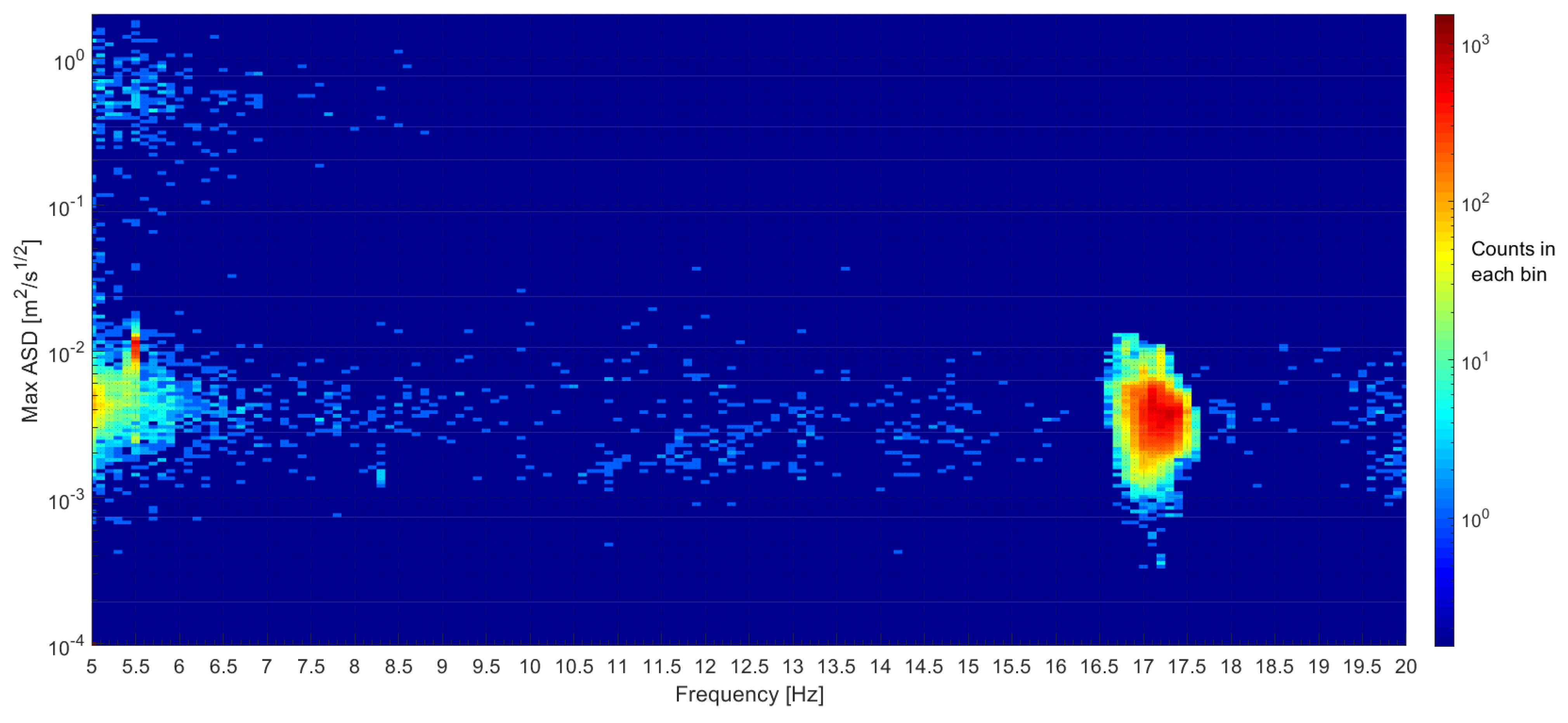
In Figure 6 a spectral histogram of the data is shown, i.e., a two–dimensional distribution of max(ASD) values vs. dominant frequencies. Apparently, there are two main frequencies at which ASD maxima accumulate: ca. 5–6 Hz and ca. 17 Hz. The first one is characterized by strong day–night periodicity. As for the 5.5 Hz wave, its peak in frequency domain is very sharp, while for 17.1 Hz it is more blurred.

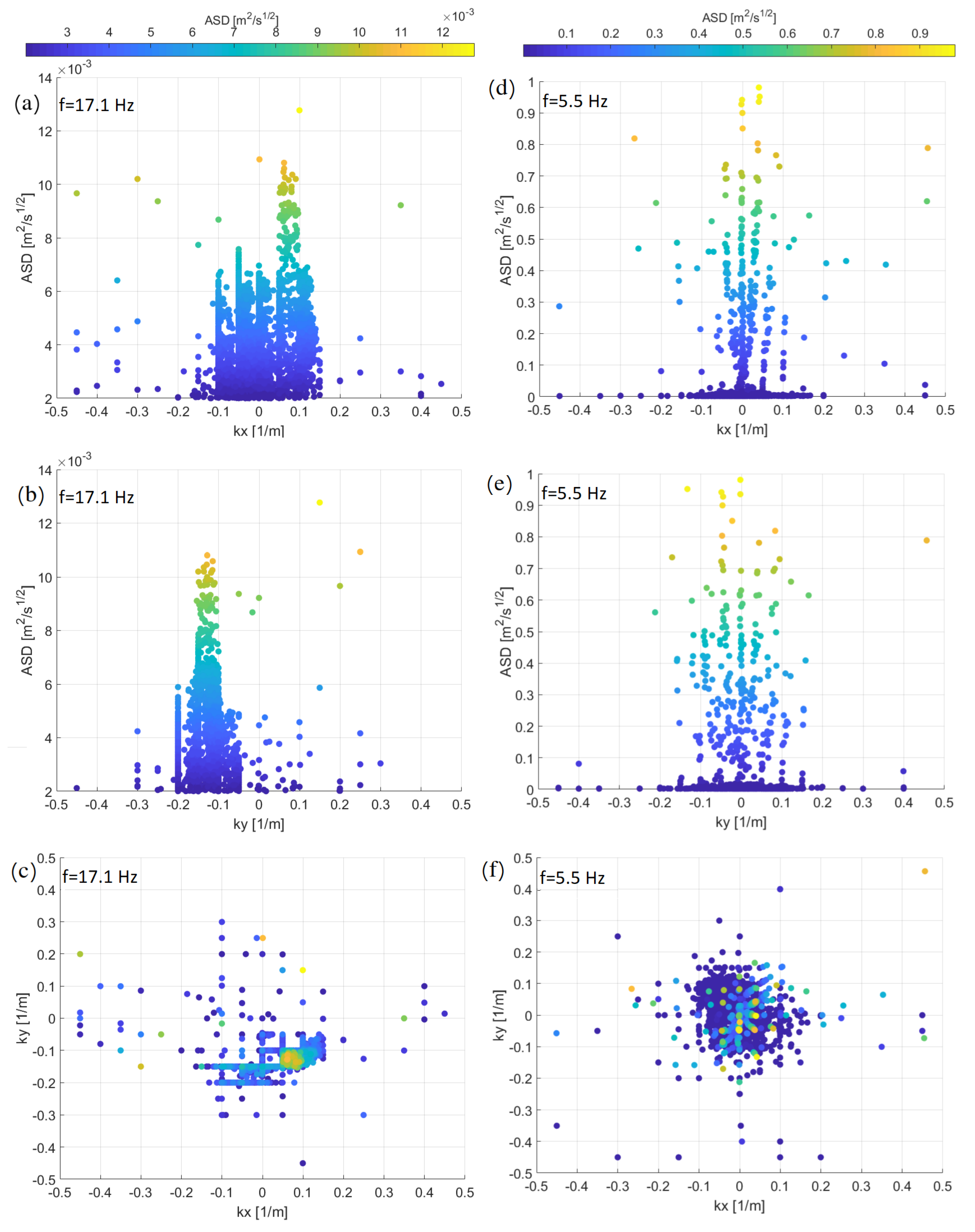
Using methodology described in Section 3.3 coordinates of each max(ASD) in the wave–vector space, for particular frequencies and 20-s periods of the measurement, were found. Results are shown in Figure 7a–c for 17.1 Hz and Figure 7d–f for 5.5 Hz.

For the sake of clarity, the results are projected on $XZ$, $YZ$, and $XY$ surfaces, where X and Y correspond to $k_x$ and $k_y$, respectively, and Z reflects ASD. To account for measurement and computation uncertainty we set a lower limit for max(ASD) to $0.5\%$ of the maximal ASD value for all data, which was equal to $2.13{\mathrm{m}}^2/{\mathrm{s}}^{1/2}$.

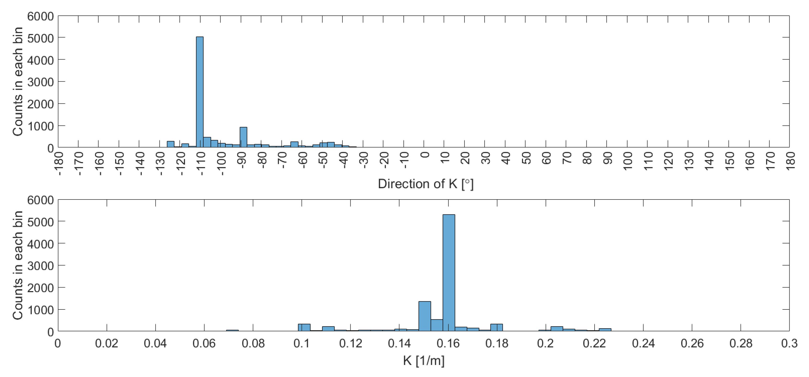
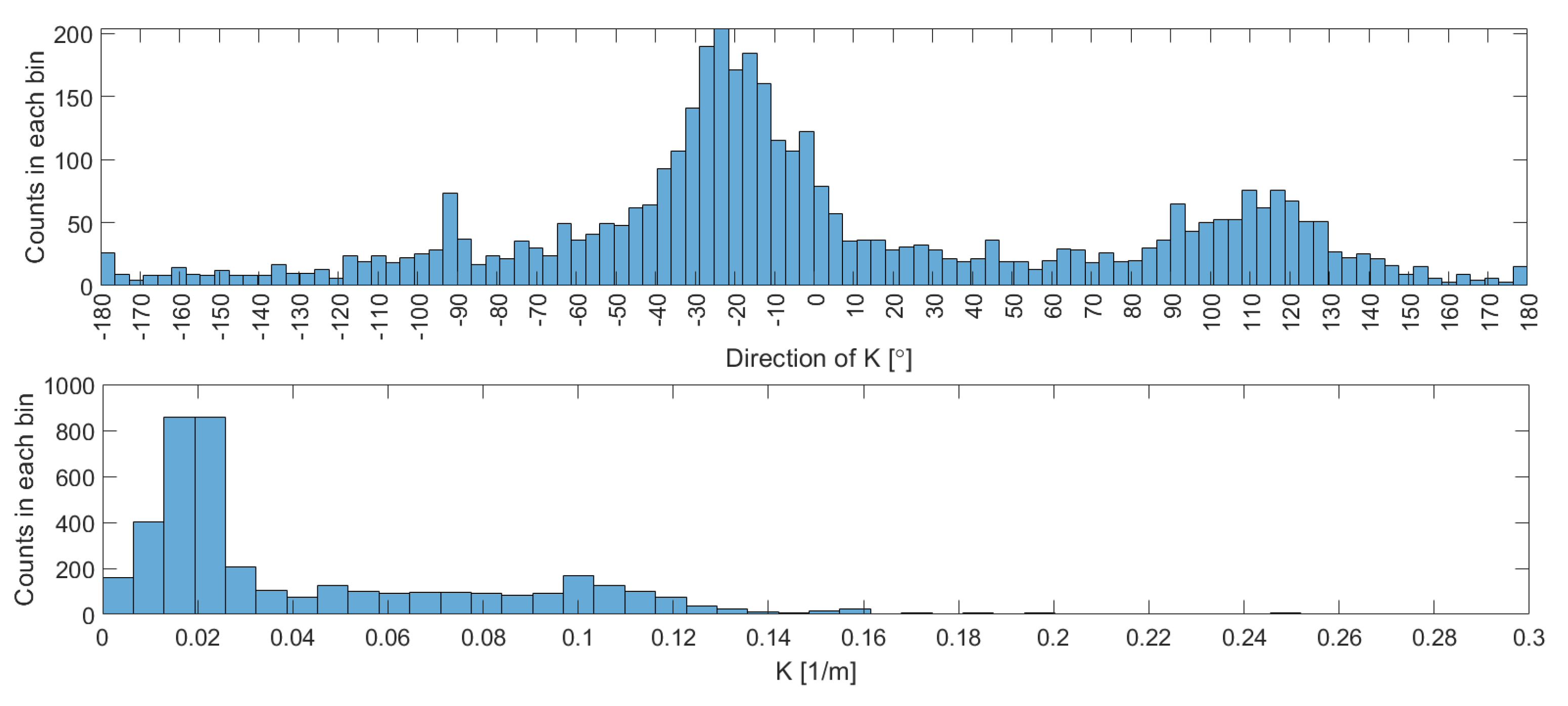
Figure 8 and Figure 9 for frequencies 17.1 Hz and 5.5 Hz, respectively, are histograms of wave direction and wavenumber. $0^{°}$ on upper plots does not indicate cardinal direction, but direction of X axis in the seismometer coordination system presented in

Table A1. Coordinates of the seismometers with respect to the Virgo test mass.

No.	$\mathit{x}\left[\mathit{m}\right]$	$\mathit{y}\left[\mathit{m}\right]$	$\mathit{z}\left[\mathit{m}\right]$
1	−2996.1855	3.3109	−3.4011
2	−2998.6876	7.1706	−3.4071
3	−2999.3596	3.2421	−3.4008
4	−3003.9149	7.8757	−3.4227
5	−3003.0811	3.2749	−3.4150
6	−3005.9728	7.7190	−3.4288
7	−3006.2434	3.3279	−3.4237
8	−3010.3192	7.9888	−3.4437
9	−3012.1375	3.3488	−3.4299
10	−3014.7164	7.5541	−3.4490
11	−3017.8701	4.2944	−3.4613
12	−3014.9770	−0.0874	−3.4426
13	−3017.9104	−4.0994	−3.4595
14	−3015.1017	−7.3702	−3.4573
15	−3013.7171	−3.1819	−3.4287
16	−3011.1778	−6.0311	−3.4400
17	−3009.9611	−3.1498	−3.4302
18	−3005.5196	−6.1313	−3.4285
19	−3005.9568	−3.1540	−3.4234
20	−3003.6825	−6.6868	−3.4195
21	−3000.1694	−3.4201	−3.4149
22	−2999.4935	−5.4172	−3.4146
23	−2996.6250	−3.3377	−3.4085
24	−2999.3105	2.7366	−3.3156
25	−3002.9757	2.6436	−3.3247
26	−3006.8761	2.7944	−3.3304
27	−3010.9353	2.8204	−3.3416
28	−3013.8210	2.3477	−3.3491
29	−3013.6882	−2.6371	−3.3435
30	−3011.2803	−2.5983	−3.3446
31	−3006.4946	−2.6779	−3.3386
32	−3002.6733	−2.5689	−3.3296
33	−2999.6753	−2.5736	−3.3223
34	−2999.8896	0.0321	−3.3182
35	−3009.4183	0.0789	−3.3497
36	−3013.7110	−0.0613	−3.3462
37	−3012.2423	−1.1159	−6.8445
38	−3008.4083	1.4434	−6.8571

. This direction is also marked in Figure 10 in comparison with cardinal direction.

For frequency 17.1 Hz results indicate the direction $-110\pm {2.5}^{°}$ and wavenumber $|K_{17.1}|=0.158$ 1/m. Using this formula these values correspond to the seismic wave arriving from northeast with velocity $680\pm 111$ m/s. The 5.5 Hz wavefield direction is ca. $-25\pm {16.3}^{°}$ with wavenumber $|K_{17.1}|=0.02$ 1/m. These values correspond to the seismic wave arriving from northwest with velocity $1727\pm 431$ m/s.

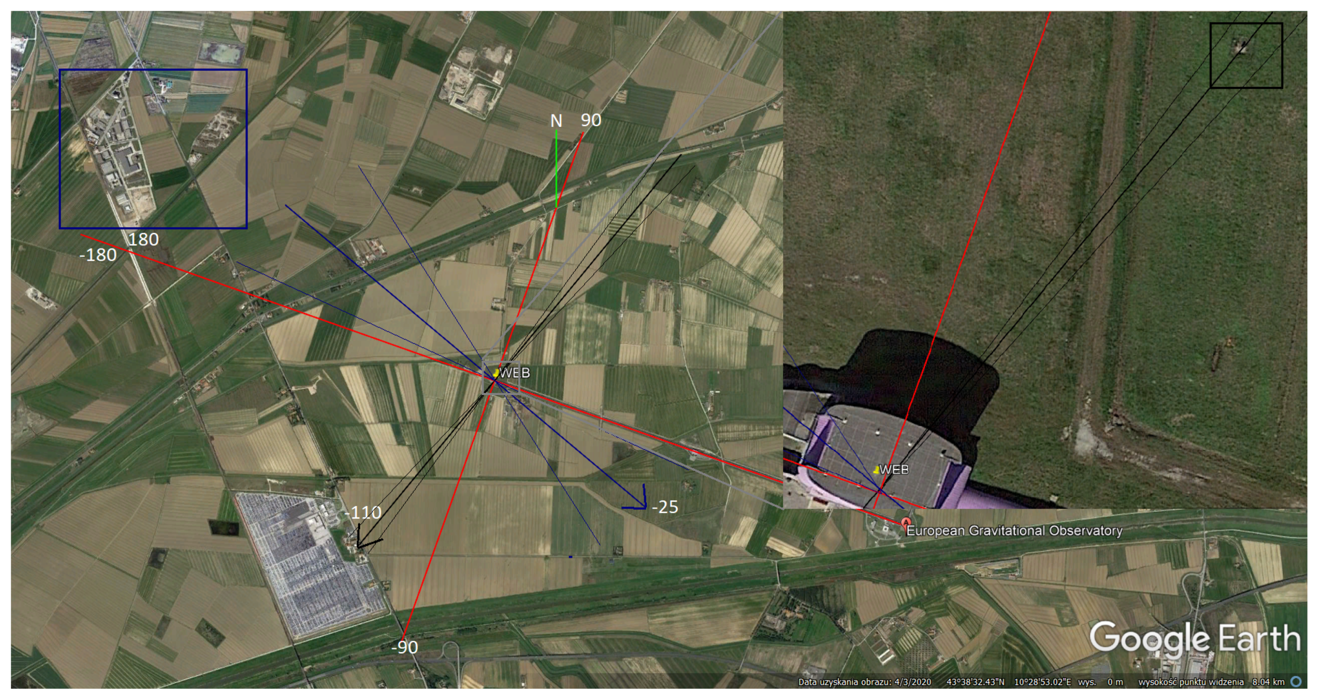
In Figure 10 the map of the vicinity of the Virgo detector with directions of waves propagation is shown. Red lines is an assumed coordination system, shifted ${19.5}^{°}$ clockwise to cardinal north. Blue lines indicate direction of 5.5 Hz wave with errors. The area in blue rectangle, i.e., an industrial complex 2.5 km away from the WEB, may be a source of this wave. Black color indicates direction of 17.1-Hz wave. In the top–right corner of Figure 10 a zoom of the vicinity of the WEB is shown, with a potential source of 17.1 Hz wave marked (black rectangle), ca. 100 m away for the WEB.

5. Discussion

Using the data from the experiment conducted between 24 January 2018 and 6 February 2018 collected by the system of seismometers inside the west–end building of Virgo, we made a seismic analysis of the nearby area.

We searched for the seismic waves with a frequency from 5 to 20 Hz. Two dominant frequencies were detected and associated with possible sources, the first one is present most of the time, the second one appears primarily during daytime. First observed dominant frequency is 17.1 Hz. The direction of this wave is $-110\pm {2.5}^{°}$, i.e., it was arriving from northeast, with velocity $680\pm 111$ m/s. In Figure 10 top–right corner a small object located ca. 100 m from WEB matches the found wave direction. It is located exactly at the found wave direction. However, this is a technical construction used for controlling the hydrology of the terrain and it is not a likely source of the 17.1-Hz wave. For the most likely source of the 17.1-Hz wave see [29].

Seismic waves at the frequency 5.5 Hz appear associated with daily human activity. They dominate between 6 a.m. and 6 p.m. every day and move with velocity $1727\pm 431$ m/s. A direction of this waves is not strict, ca. $-25\pm {16.3}^{°}$. A supposed origin of the waves is human activity and heavy traffic activity in the nearby industrial complex. Previous studies indicated another antropogenic source of the noise at the frequency 4–10 Hz: nearby high–traffic elevated roads [23,25]. The directional analysis we did is not fully consistent with such an interpretation.

The velocities given above are typical of dispersion media, i.e., the wave with lower frequency moves faster, and agree with the predictions of one of the models from [8]. The typical velocity of Rayleigh waves in metals is 2–5 km/s, while in soil 50–700 m/s for shallow waves (under 100 m) and 1.5–4 km/s for depth over 1 km [36].

Future Work

The method of seismic–wave detection in the Virgo WEB presented above, can detect specific waves that pass through the building. The main advantage of the method is that it provides the full information about the waves that pass through the measuring system (frequency, velocity, direction, and amplitude) with small loss of the information from the seismometers, as it does not use data averaging.

The concept of minimization of Newtonian noise in the Virgo GW signal is based on monitoring sources of gravitational field perturbations. These perturbations are caused by local changes of density in the vicinity of the test masses. A commonly proposed method for the reduction of Newtonian noise is based on Wiener filters, which have been already applied for the reduction of other noises in GW detectors [37]. The parameters of seismic waves found in this work can be used to fit correlation models of the Wiener filter [9].

The analysis conducted herein can be applied to other Virgo experimental areas, where the other test masses are located. For the west–end building itself the data were collected for more than one year; in the north–end building and central building a system of sensors is going to be installed as well. Complementarily to seismometer arrays, infrasound microphone arrays are going to be used for a characterization of the sources of gravitational field fluctuations caused by pressure changes. In particular, a detailed analysis of the frequencies below 10 Hz would be important, as for 1.7 Hz a significant noise coming from the nearby wind farm is observed [24].

One of the problems that needs solving when we use the spatio–temporal spectral analysis method is how to distinguish between the real waves and the noise. For instance, some threshold values may be used for this purpose [38,39]. However, in this article we focused on the dominant frequencies observed in the signals. The sensitivity is limited by the computational noise due to the non–uniform grid and is likely to be limited to waves with the amplitude not larger than 10% of the dominant wave as seen from Figure 1, where the signal is ca. 10 times larger in amplitude than the noise. Moreover, the issue of spatial aliasing should be resolved, e.g., by applying the window function also for the spatial dimensions (cf. Section 3). On top of that, we may consider the use of overlapping time periods when calculating the spectra, to improve the accuracy and relevance of the results.