Hard Negative Samples Contrastive Learning for Remaining Useful-Life Prediction of Bearings


1
School of Computer and Information, Hefei University of Technology, Hefei 230601, China
2
Shanghai Aerospace Control Technology Institute, Shanghai 201109, China
3
The Institute of Industry and Equipment Technology, Hefei University of Technology, Hefei 230601, China
*
Author to whom correspondence should be addressed.
Lubricants 2022, 10(5), 102; https://0-doi-org.brum.beds.ac.uk/10.3390/lubricants10050102
Submission received: 15 April 2022
/
Revised: 12 May 2022
/
Accepted: 18 May 2022
/
Published: 21 May 2022
(This article belongs to the Special Issue Advances in Bearing Lubrication and Thermal Sciences)
Abstract
:In recent years, deep learning has become prevalent in Remaining Useful-Life (RUL) prediction of bearings. The current deep-learning-based RUL methods tend to extract high dimensional features from the original vibration data to construct the Health Indicators (HIs), and then use the HIs to predict the remaining life of the bearings. These approaches ignore the sequential relationship of the original vibration data and seriously affect the prediction accuracy. In order to tackle this problem, we propose a hard negative sample contrastive learning prediction model (HNCPM) with encoder module, GRU regression module and decoder module, used for feature embedding, regression RUL prediction and vibration data reconstruction, respectively. We introduce self-supervised contrast learning by constructing positive and negative samples of vibration data rather than constructing any health indicators. Furthermore, to avoid the subtle variability of vibration data in the health stage to aggravate the degradation features learning of the model, we propose the hard negative samples by cosine similarity, which are most similar to the positive sample. Meanwhile, a novel infoNCE and MSE-based loss function is derived and applied to the HNCPM to simultaneously optimize a lower bound on mutual information of the positive and negative sample over life cycle, as well as the discrepancy between true and predicted values of the vibration data, such that the model can learn the fine-grained degradation representations by predicting the future without any HIs as labels. The HNCPM is validated on the IEEE PHM Challenge 2012 dataset. The results demonstrate that the prediction performance of our model is superior to the state-of-the-art methods.
1. Introduction
Bearings undergo an irreversible degradation process during use that eventually leads to bearing breakdown. Via predicting the Remaining Useful Life (RUL) of bearings, one can avoid missing the best time for maintenance [1] and remanufacturing [2]. However, in realistic industrial scenarios, due to noise, variation in life cycle and other prediction uncertainties [3], RUL prediction is a challenging issue [4].
Generally, RUL prediction of bearings is implemented in two different strategies [5]: physically based approaches [6,7,8] and data-driven [9,10,11,12] approaches. Compared with the former, data-driven RUL methods use historical data directly to build prediction models, which avoids the difficulties in modeling of the physical model and has become the prevalent approach in recent years [13,14,15]. For instance, Xia et al. used a denoising autoencoder to classify the original signal into different degradation stages and extracted representative features directly from the original signal using DNN. Then they obtained RUL values for each stage using deep regression models [16]. Guo et al. proposed a recurrent neural-network-based health indicator(RNN-HI) with fairly high monotonicity and correlation values, which is beneficial to bearing RUL prediction [17].
Among several data-driven methods, deep learning-based methods obtained considerable results in bearing RUL prediction, which do not require manual feature design and build an end-to-end deep neural network to map the relationship between the degradation process and the original sensory data [18].
The existing deep-learning-based approaches usually construct health indicators (HI) that can represent the degradation trend of bearing performance, then predict the degradation trend using deep-learning regression models [18]. The effectiveness of these approaches largely relies on these HIs accurately modeling the degradation trend of bearings. However, in real-world industrial applications, the degradation processes of different bearings are diverse. The existing HIs usually describe the overall trend of the whole life cycle, but fail to represent the changes of local details. Using these inappropriate HIs as model input will directly restrict the prediction performance of the model.
Noted that the original time-domain vibration data of bearings contains the sequential relationship with respect to the degradation trend of bearings, thus predicting that the original vibration data, instead of any designed HI, can more accurately evaluate the model performance. However, the time-domain vibration data changes slightly in the health stage; the existing well-developed methods are less capable of capturing the latent features of the bearing data at this stage.
To circumvent the aforementioned problems, we propose an end-to-end hard negative sample contrastive learning prediction model, termed HNCPM. We construct a three-layer, one-dimensional convolutional-based encoder module to map the high-dimensional original vibration data to a low-dimensional feature space to facilitate the model’s computation. Next, we adopt a Gated Recurrent Unit with a decoder module in this feature space to learn the sequence relationship of vibration data for RUL prediction. Importantly, the HNCPM introduces self-supervised contrastive learning to construct positive and negative samples of vibration data, rather than supervised leaning via any HI labels. Considering there is no significant variability between the positive and negative samples in the health stage, thus we select the most similar negative sample to the positive sample as the hard negative sample via cosine similarity, to improve the fine-grained feature identification of the model. Finally, we design the novel loss function of the model combining the Mean Square Error(MSE) with infoNCE [19] for self-supervised training from the original vibration data.
The main contributions of this work are summarized as follows:
- Unlike existing supervised RUL prediction methods, this study explores a more practical self-supervised-leaning RUL prediction method that directly learns the sequence relationship from the original vibration data instead of using any HIs as labels for the model supervised training. We propose the HNCPM with the encoder module, GRU regression module and decoder module, respectively used for feature embedding, regression RUL prediction and vibration data reconstruction.
- To encounter this dilemma that the subtle variability between the positive and negative samples in the healthy stage makes the model fail to learn the latent sequence features, we select the negative sample that is most similar to the positive sample as the hard negative sample. Correspondingly, we design a novel loss function combining the MSE with infoNCE loss to improve the fine-grained feature representation of the model.
- The performance of the proposed HNCPM is comprehensively evaluated on the IEEE PHM Challenge 2012 dataset. The comparative experimental results show that the HNCPM is superior for the excellent prediction accuracy than the state-of-the-art methods with respect to different bearings.
2. Related Works
2.1. Deep-Learning-Based Approaches for Rul Prediction
The existing deep-learning-based approaches usually include two steps: constructing the bearing HIs for model training that can represent the degradation trend of bearing performance, and designing the deep learning regression models to predict the degradation trend (usually the HIs).
In terms of model design, it generally includes: CNN [20], RNN [21] and AE [22]. Xu et al. used the SAE to extract features of bearing data to construct HI [23]. Wang et al. [24] applied deep separable convolutional networks to learn high-level representations from the original signal and then predict RUL. Wu et al. [25] proposed Deep Long Short-Term Memory (DLLSTM) networks, and Han et al. proposed a Transferable Convolutional Neural Network(TCNN) to accurately predict the bearing RUL under different failure behaviors [26].
The common model structure can no longer fulfill the demand of researchers for superior prediction, and many recent studies have combined the advantages of different models to propose model variants. For instance, Luo et al. proposed a novel convolution-based attention mechanism bidirectional long and short-term memory (CABLSTM) network to achieve the end-to-end lifetime prediction of rotating machinery [27]. Meng et al. proposed CLSTM by conducting convolutional operation on both the input-to-state and state-to-state transitions of the LSTM to learn high-level features in the time-frequency domain for RUL prediction [28].
With respect to the HI construction, i.e., the RUL labels, since the damage extent of bearings cannot be directly observed, the RUL labels are almost unavailable in real-world scenarios. Hence, there is no uniform criterion of HI construction for RUL prediction models. The existing studies usually extracted the different fault characteristics from the original sensory signal. She et al. [29] proposed a health indicator construction method based on a Sparse Auto-encoder with a Regularization (SAEwR) Model for rolling bearings. Zhang et al. used the summation of the mean maximum radius of the different datasets divided by the k-means clustering algorithm as the health indicator, and then used the local outlier coefficient algorithm to eliminate the outliers’ influence [30]. Li et al. designed the generative adversarial network to learn the data distribution in the health states of machines, using the output of the discriminator as HI [31].
In summary, the performance of the existing HIs-based deep-learning approaches heavily relies on whether the HIs are constructed properly. Nevertheless, the models usually fail to represent the changes of local details, while capturing the overall gradation trend of the whole life-cycle of bearings, which restricts the prediction performance of the models.
Therefore, in this paper we introduce self-supervised contrastive learnin, directly using the original vibration data, rather than any HIs, to learn the sequential relationship with respect to the degradation trend of bearings.
2.2. Contrastive Learning
Self-supervised learning is committed to avoiding the manually annotating large-scale datasets by setting up pretext tasks to learn data representations [32,33,34]. The learning process is unsupervised and the trained model can be used for multiple downstream tasks. Among self-supervised learning, contrastive learning is the most widely concerned. It uses discriminative modeling to learn useful representations of unlabeled data. Several contrastive learning models, e.g., MoCo [35], SimCLR [36] and BERT [37] provide competitive results in comparison with supervised learning models within the pretext task of image classification or next-sentence prediction.
Specifically, contrastive learning is a discriminative method that aims to compact the similar samples and discriminate the dissimilar samples [38]. The models include: similarity and dissimilarity distributions for sampling positive and negative samples of the query, one or more encoders for each data pattern, and comparative loss functions for evaluating a batch of positive and negative pairs.
Given a set of n samples, for any input sample x, q is the encoded representation of x, function , denote as a positive and negative sample of the sample x.
s is a measure of the similarity between the embedded vectors, or it can be a calculation of the distance between the vectors.
To the best of our knowledge, there are limited studies that introduce contrastive learning to the RUL prediction. Mohamed Ragab et al. [39] propose a contrastive adversarial domain adaptation (CADA) method for cross-domain RUL prediction, which transfers knowledge for RUL prediction from one condition(distribution/domain) to another. That is no longer the problem dealt with in this paper. Our paper aims to discuss an unsupervised RUL prediction approach to learn degradation representations from original vibration data by using certain contrastive learning models.
Furthermore, with regard to existing contrastive learning approaches, the positive samples generated by data enhancement of the original data (e.g., rotating, segmenting), while samples are not generated from the same view, are negative samples from each other. Such approaches of constructing samples ignores the role of negative samples in model training. In fact, negative samples can teach learning models to correct their errors faster in representation learning. More importantly, the information-rich counterexamples are intuitively those that map far away from the positive sample but are closer to the positive sample than to other negative samples [40].
Inspired by this idea, in this paper we construct positive and negative samples based on the different temporal relationship of the vibration data, enabling the model to learn the sequence features by discriminating whether the temporal relationship of the vibration data is correct or not. Moreover, we construct hard negative samples to express the most similar to the positive sample to improve the fine-grained feature representation of the model.
3. Proposed Method
As shown in Figure 1, the complete framework of the proposed method includes construction of the positive sample and hard negative samples, the hard negative sample contrastive learning prediction model and corresponding optimization function.
3.1. Positive Sample and Hard Negative Sample Construction
Without loss of generality, we denote that the original vibration data of bearing is , the positive sample dataset is , , and , where and , respectively. The timestep is the timestep of the vibration sequence. In this paper, it is set to six.
Random can form a negative sample with . We use the cosine similarity to calculate the negative sample with the highest similarity to .
when = , w is maximum, at which and form a hard negative sample, and and form a positive sample. We use to construct the hard negative sample dataset , denote , .
Given a dataset of k random samples containing one sample from and samples from , corresponding prediction labels, the positive and negative sample labels are and , respectively. Initialize the positive and hard negative sample label set .
.
3.2. Hard Negative Contrastive Prediction Model (Hncpm)
After the positive and negative sample pairs are generated based on the original vibration data of bearing , the feature sequence are extracted through an encoder composed of three layers of a one-dimensional convolutional network, which compresses the original vibration data into a low-dimensional feature space. Then, we use a gated recurrent unit as a regression module to learn the sequence relationship of the feature sequence. Finally a decoder composed of three fully connected layers predicts the vibration data in future time-periods (i.e., RUL).
Unlike the existing supervised learning model to predict the HI labels for RUL, the HNCPM directly predicts the vibration data in future time-periods with the purpose of allowing the model to better fit the time domain graph curve of the original vibration data, so the potential representation of the context is captured in the gated recurrent units and the final prediction results are obtained through a decoder. The model structure is shown in Table 1.
The feature encoder module composed of three convolutional layers is formulated as follows:
where ⊗ is the valid cross-correlation operator and is the weight.
The regression module uses gated recurrent units, which can effectively suppress gradient disappearance or exploding gradient when capturing long sequence data association. It is better than traditional RNN and has less computational complexity than LSTM.
where is the hidden state at time i. , , are the reset, update, and new gates, respectively. ,, and W are the weight, weight, weight, respectively.
After the regression module, the decoder consisting of three fully connected layers is used for decoder enhancement of the dimensionality of , with the following output:
where is the weight of the fully connected layers.
3.3. Optimization Function
The loss function of the model in this paper consists of two parts: (1) the regression loss function ; (2) the contrastive prediction loss function .
The regression loss function uses the mean square error to predict the bearing data of the next time period based on the vibration data of the previous time segment. The input dataset is for the model training. The loss function is as follows:
where N is the total number of samples.
The contrastive prediction loss function is the loss function [19], which is commonly used in contrastive learning. Feed set C into HNCPM, the output is .
According to previous study [19], the higher the density ratio function , the larger the mutual information of and , and the more capable of predicting by . The formula is as follows:
measures the degree of similarity between the predicted result and .
where ⊙ is the Hadamard multiplier.
Finally, the total loss function of HNCPM is as shown:
where is the hyperparameter.
The pseudo code of the algorithm for training is shown in Algorithm 1.
| Algorithm 1 Hard Contrastive Prediction Model |
| Input: original bearing samples: . positive samples: , , , . hard negative samples: , , select by (2). F consists of encoder, gated recurrent unit, decoder. is the proposed model parameters. is the test bearing data |
|
| Output: the model prediction |
4. Experimental Section
In this section, we use the IEEE PHM Challenge 2012 bearing dataset to validate the effectiveness of the proposed method. The Mean Absolute Error (MAE) and Root Mean Square Error(RMSE) are selected as indicators to evaluate the model performance. The smaller the value of MAE and RMSE, the more superior the RUL model is. The MAE and RMSE, respectively, are expressed as follows.
where denotes the true value of the sample, denotes the predicted value, and N is the total number of samples.
4.1. Data Description
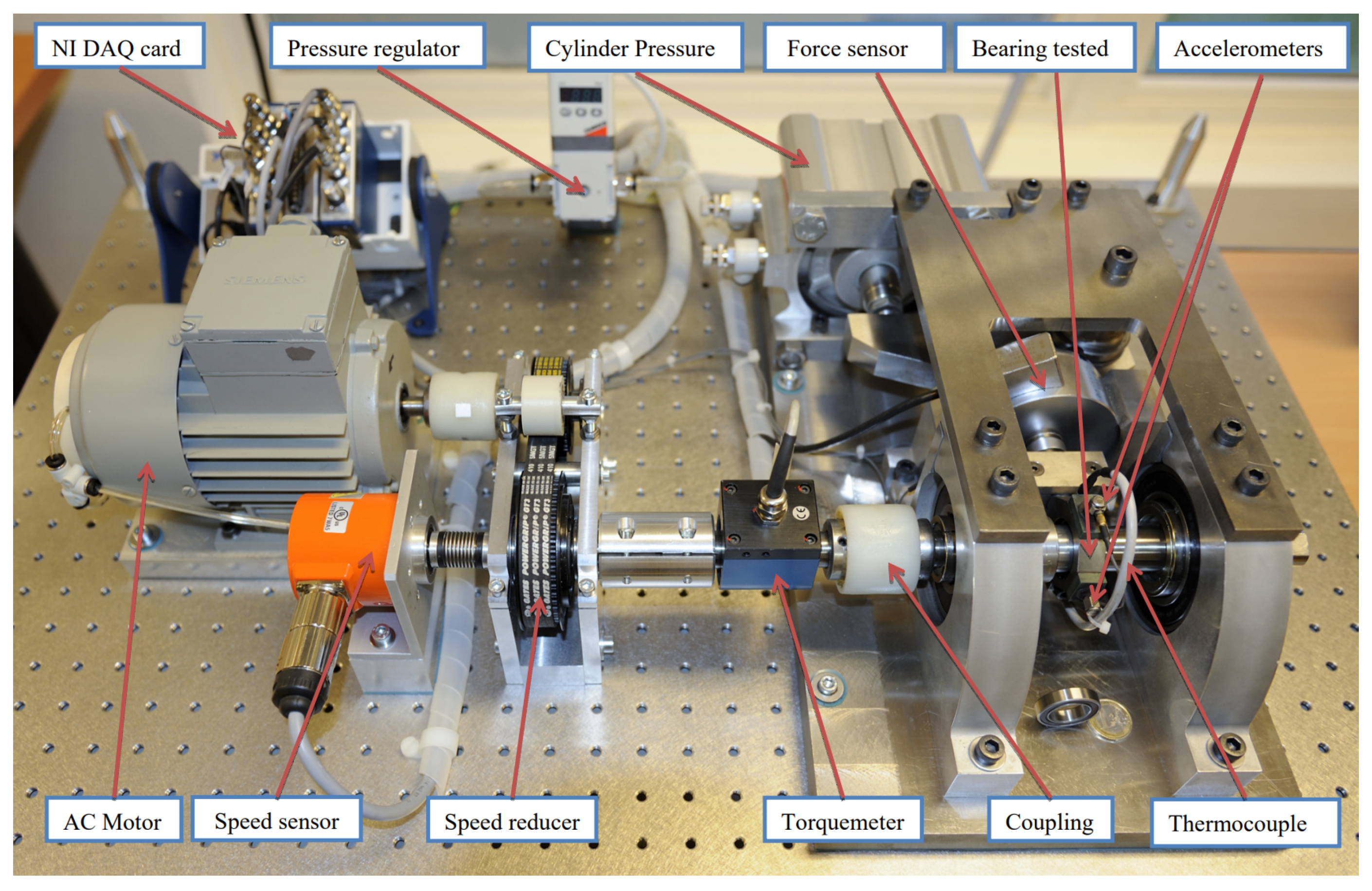
As shown in Figure 2, The PRONOSTIA test platform contains a rotating part, a load part, and a data collection part. The motor power is 250 W. The power is transferred to the bearing by the axis of rotation. The accelerated degradation experiments was conducted on this platform to generate the run-to-failure vibration signal. The acceleration sensors are placed in horizontal and vertical directions to collect vibration signals under three working conditions. The sampling frequency is 25.6 kHz. The vibration signal is recorded every 10 s, and each acquisition lasts 0.1 s. For example, under the first working condition, the vibration signals of six bearings were collected, namely, bearing 1_2, bearing 1_3, bearing 1_4, bearing 1_5, bearing 1_6 and bearing 1_7. The motor’s rotation speed is 1800 rpm, and the load is 4000 N.
In the following different experiments, the vibration signals of bearing 1_2 are the training set, while bearing 1_4, bearing 1_5, bearing 1_6, bearing 1_7, bearing 2_3, bearing 2_4, bearing 2_5, and bearing 2_6 are used as the testing set, respectively, as shown in Table 2.
4.2. Weighting Factor Analysis
In Equation (12), the weights of the loss function are empirically determined. Hence, we perform several experiments to discuss their influence on the model performance.
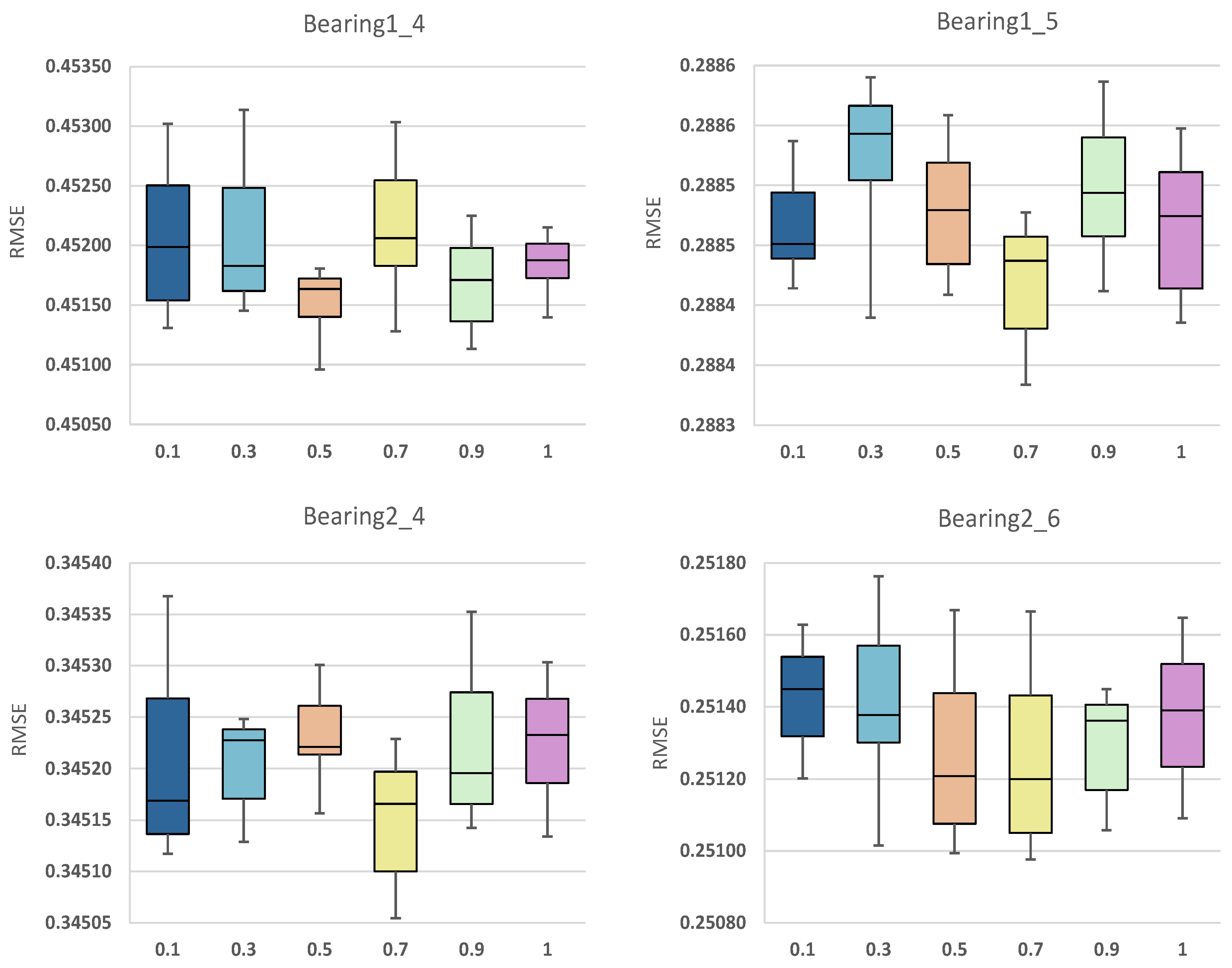
Herein, the experiments are taken as 0.1, 0.3, 0.5, 0.7, 0.9, 1, respectively. Bearing 1_4, bearing 1_5, bearing 2_4, and bearing 2_6 are used as the test set and RMSE is used as the model predictive ability index. For each series of experiments, we repeat the experiment ten times and report the average performance. Figure 3 depicts the box plot of RUL prediction results for four different bearings at different .
When , the weight of in the total loss L is too small and plays a low optimization role in the model, resulting in poor prediction results in bearing 1_4, bearing 2_4, bearing 2_6. In contrast, when , the model is overly concerned with the fine-grained recognition of vibration data, resulting in overfitting; thus the model has an unsatisfactory generalization effect in testing bearing 1_5, bearing 2_4, and bearing 2_6. When , our method performs best on bearing 2_6, and the maximum and minimum values of RMSE are lower than other weights. It also has the same superiority on bearing 1_5 and bearing 2_4 compared with other weights. Considered comprehensively, the prediction accuracy of the model is satisfactory when .
4.3. Ablation Experiments
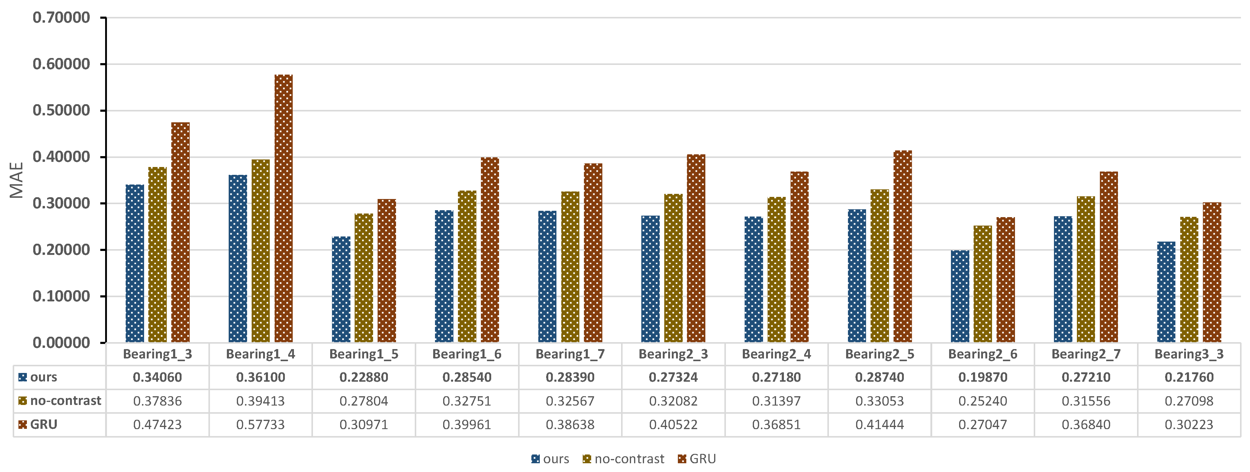
In this section, we perform ablation experiments to verify the contribution of each module in our model. We keep the model structure unchanged but without contrast learning (termed as no-contrast), and GRU model without encoder and decoder modules (termed as GRU) to compare with HNCPM. MAE is used as the predictive ability index of the models. The experimental results are demonstrated in Figure 4.
HNCPM has the best superiority on bearing 2_6, which is 0.05 lower than the no-contrast model and 0.07 lower than the GRU model. In addition, the model has the largest MAE value on bearing 1_4, which is 0.03 and 0.22 lower than the no-contrast and GRU model, respectively.
Moreover, compared to the GRU model, the no-contrast model has a better prediction performance because it contains the feature extraction layer to extract high-dimensional degradation features from the original vibration data, facilitating the RUL regression prediction. However, no-contrast ignores latent sequence features during the training, while HNCPM introduces contrast learning to improve the fine-grained model training and improve the prediction efficiency compared to no-contrast. Overall, the prediction results on all bearing data indicate that the proposed HNCPM method is significantly superior to the other two models.
4.4. Comparison with State-of-the Art Methods
In this section, our proposed HNCPM is compared with the state-of-the-art novel rolling bearing health-prediction methods based on CNN and BiLSTM models [41], and BiLSTM with attention mechanism [42]. In addition, we compare general encode and regression model combinations (i.e., SAE+GRU, CNN+LSTM) to evaluate the model prediction performance. MAE is used as the predictive ability index of the models. The overall RUL prediction results using the aforementioned models are depicted in Figure 5.
It can be seen that SAE model has the worst performance. It is well known that SAE has strong signal denoising ability, but its feature extraction ability in time series data is not as good as CNN. Attention increases the weight of important features, but it also ignores the bearing sequence information that is masked by noise, which results in an unstable prediction performance on multiple bearings. Therefore, the performances of CNN-based models are superior to the other model.
In addition, The MAE value of CNN+BiLSTM is, on average, 0.2 lower than CNN+LSTM, as the BiLSTM improves the model prediction ability through backward prediction of past bearing data through future data. However, BiLSTM has one more backward hidden layer relative to LSTM, which boosts the number of model parameters and increases the model overhead, and the prediction performance is not as efficient as HNCPM.
Compared with the other models, HNCPM has the smallest MAE value at bearing 2_6 and is 0.06 lower than the second-best model (i.e., CNN+BiLSTM). Meanwhile, HNCPM has the largest MAE value at bearing 1_4, i.e., 0.361, but it is also at least 0.01 lower than the other models. The experiments demonstrate that HNCPM has a superior performance in RUL prediction.
4.5. Prediction Results Visualization
In this section, unlike the existing RUL prediction techniques which predict the degradation index (DI) [41] or the root mean square(RMS) [42] from the vibration data, we use manifold learning to visualize the fitting curve between the prediction and the original data to evaluate the prediction performance of the model more intuitively. We use the vibration data of the first 1800 time points to predict the remaining vibration data on bearing 1_3 and bearing 2_3, respectively. Figure 6a,b are the original time domain vibration data of bearing 1_3 and bearing 2_3, respectively. Each time point of vibration data is 2560 in dimension. In order to illustrate the prediction performance more intuitively, TSNE is used to transform the 2560 dimension data of each time point into 1 dimension on bearing 1_3 and bearing 2_3, as in Figure 6c,d. The blue curve is the real vibration data; the orange curve is the prediction data.
From Figure 6c, some of the prediction data are biased with the real data curve in the rapid degradation stage because the vibration data of bearing 1_3 changes drastically at the end of life, which is difficult for the prediction of the model. Meanwhile it can be found from Figure 6d that the vibration data of bearing 2_3 changes slowly in the whole life-cycle; thus, the prediction curve of model is more feasible to fit the real data curve.
5. Conclusions
In this article, we proposed a novel RUL prediction approach of bearings, termed HNCPM, which introduces self-supervised contrast learning to directly use the original vibration data for model training rather than any HIs as the RUL label, improving the model’s ability to extract sequential relationships from the original data. Meanwhile, we construct a hard negative sample and further design a novel loss function, combining the MSE with infoNCE loss to address the dilemma for the model to learn fine-grained degradation features due to the insignificant variation of positive and negative samples in the bearing health stage. Our experimental results demonstrate the superiority of the proposed HNCPM method for RUL prediction and the fine fit of the model predictions to true RUL observed by manifold learning.
Author Contributions
Conceptualization, J.X.; writing—original draft preparation, L.Q.; formal analysis, W.C.; validation, X.D. All authors have read and agreed to the published version of the manuscript.
Funding
This work was supported in part by the National Key Research And Development Plan under Grant 2018YFB2000505, in part by the Key Research and Development Plan of Anhui Province under Grant 202104a04020003, and in part by the Fundamental Research Funds for the Central Universities under Grant PA2021KCPY0045.
Institutional Review Board Statement
Not applicable.
Informed Consent Statement
Not applicable.
Data Availability Statement
Public datasets used in our paper: https://github.com/wkzs111/phm-ieee-2012-data-challenge-dataset (accessed on 10 April 2022).
Conflicts of Interest
The authors declare no conflict of interest.
References
- Uckun, S.; Kai, G.; Lucas, P. Standardizing research methods for prognostics. In Proceedings of the International Conference on Prognostics & Health Management, Denver, CO, USA, 25 March 2008. [Google Scholar]
- Zhang, M.; Amaitik, N.; Wang, Z.; Xu, Y.; Maisuradze, A.; Peschl, M.; Tzovaras, D. Predictive Maintenance for Remanufacturing Based on Hybrid-Driven Remaining Useful Life Prediction. Appl. Sci. 2022, 12, 3218. [Google Scholar] [CrossRef]
- Jardine, A.; Lin, D.; Banjevic, D. A review on machinery diagnostics and prognostics implementing condition-based maintenance-ScienceDirect. Mech. Syst. Signal Process. 2006, 20, 1483–1510. [Google Scholar] [CrossRef]
- Heng, A.; Zhang, S.; Tan, A.C.; Mathew, J. Rotating machinery prognostics: State of the art, challenges and opportunities. Mech. Syst. Signal Process. 2009, 23, 724–739. [Google Scholar] [CrossRef]
- Lei, Y.; Li, N.; Guo, L.; Li, N.; Yan, T.; Lin, J. Machinery health prognostics: A systematic review from data acquisition to RUL prediction. Mech. Syst. Signal Process. 2018, 104, 799–834. [Google Scholar] [CrossRef]
- Li, N.; Gebraeel, N.; Lei, Y.; Bian, L.; Si, X. Remaining useful life prediction of machinery under time-varying operating conditions based on a two-factor state-space model. Reliab. Eng. Syst. Saf. 2019, 186, 88–100. [Google Scholar] [CrossRef]
- Prakash, G.; Narasimhan, S.; Pandey, M. A probabilistic approach to remaining useful life prediction of rolling element bearings. Struct. Health Monit. 2019, 18, 466–485. [Google Scholar] [CrossRef]
- Rai, A.; Kim, J.M. A novel health indicator based on the Lyapunov exponent, a probabilistic self-organizing map, and the Gini-Simpson index for calculating the RUL of bearings. Measurement 2020, 164, 108002. [Google Scholar] [CrossRef]
- Jiang, J.R.; Lee, J.E.; Zeng, Y.M. Time Series Multiple Channel Convolutional Neural Network with Attention-Based Long Short-Term Memory for Predicting Bearing Remaining Useful Life. Sensors 2020, 20, 166. [Google Scholar] [CrossRef] [Green Version]
- Cui, L.; Wang, X.; Wang, H.; Ma, J. Research on Remaining Useful Life Prediction of Rolling Element Bearings Based on Time-Varying Kalman Filter. IEEE Trans. Instrum. Meas. 2019, 69, 2858–2867. [Google Scholar] [CrossRef]
- Cheng, C.; Ma, G.; Zhang, Y.; Sun, M.; Teng, F.; Ding, H.; Yuan, Y. A Deep Learning-Based Remaining Useful Life Prediction Approach for Bearings. IEEE/Asme Trans. Mechatron. 2020, 25, 1243–1254. [Google Scholar] [CrossRef] [Green Version]
- Chen, Y.; Peng, G.; Zhu, Z.; Li, S. A novel deep learning method based on attention mechanism for bearing remaining useful life prediction. Appl. Soft Comput. 2019, 86, 105919. [Google Scholar] [CrossRef]
- Shao, S.Y.; Sun, W.J.; Yan, R.Q.; Peng, W.; Gao, R.X. A Deep Learning Approach for Fault Diagnosis of Induction Motors in Manufacturing. Chin. J. Mech. Eng. 2017, 30, 1347–1356. [Google Scholar] [CrossRef] [Green Version]
- Kim, J.M.; Sohaib, M. Reliable Fault Diagnosis of Rotary Machine Bearings Using a Stacked Sparse Autoencoder-Based Deep Neural Network. Shock Vib. 2018, 2018, 2919637.1–2919637.11. [Google Scholar]
- Bienefeld, C.; Kirchner, E.; Vogt, A.; Kacmar, M. On the Importance of Temporal Information for Remaining Useful Life Prediction of Rolling Bearings Using a Random Forest Regressor. Lubricants 2022, 10, 67. [Google Scholar] [CrossRef]
- Xia, M.; Li, T.; Shu, T.; Wan, J.; de Silva, C.W.; Wang, Z. A Two-Stage Approach for the Remaining Useful Life Prediction of Bearings Using Deep Neural Networks. IEEE Trans. Ind. Inform. 2019, 15, 3703–3711. [Google Scholar] [CrossRef]
- Guo, L.; Li, N.; Jia, F.; Lei, Y.; Lin, J. A recurrent neural network based health indicator for remaining useful life prediction of bearings. Neurocomputing 2017, 240, 98–109. [Google Scholar] [CrossRef]
- Rui, Z.; Yan, R.; Chen, Z.; Mao, K.; Gao, R.X. Deep learning and its applications to machine health monitoring. Mech. Syst. Signal Process. 2019, 115, 213–237. [Google Scholar]
- Van den Oord, A.; Li, Y.; Vinyals, O. Representation learning with contrastive predictive coding. arXiv 2018, arXiv:1807.03748. [Google Scholar]
- Krizhevsky, A.; Sutskever, I.; Hinton, G.E. Imagenet classification with deep convolutional neural networks. Commun. ACM 2017, 60, 84–90. [Google Scholar] [CrossRef]
- Graves, A.; Mohamed, A.R.; Hinton, G. Speech recognition with deep recurrent neural networks. In Proceedings of the 2013 IEEE International Conference on Acoustics, Speech and Signal Processing, Vancouver, BC, Canada, 26–31 May 2013; IEEE: Piscataway, NJ, USA, 2013; pp. 6645–6649. [Google Scholar]
- Vincent, P.; Larochelle, H.; Lajoie, I.; Bengio, Y.; Manzagol, P.A.; Bottou, L. Stacked denoising autoencoders: Learning useful representations in a deep network with a local denoising criterion. J. Mach. Learn. Res. 2010, 11, 3371–3408. [Google Scholar]
- Xu, F.; Huang, Z.; Yang, F.; Wang, D.; Tsui, K.L. Constructing a health indicator for roller bearings by using a stacked auto-encoder with an exponential function to eliminate concussion. Appl. Soft Comput. 2020, 89, 106119. [Google Scholar] [CrossRef]
- Wang, B.; Lei, Y.; Li, N.; Yan, T. Deep separable convolutional network for remaining useful life prediction of machinery. Mech. Syst. Signal Process. 2019, 134, 106330. [Google Scholar] [CrossRef]
- Wu, J.; Hu, K.; Cheng, Y.; Zhu, H.; Shao, X.; Wang, Y. Data-driven remaining useful life prediction via multiple sensor signals and deep long short-term memory neural network. Isa Trans. 2020, 97, 241–250. [Google Scholar] [CrossRef]
- Cheng, H.; Kong, X.; Chen, G.; Wang, Q.; Wang, R. Transferable convolutional neural network based remaining useful life prediction of bearing under multiple failure behaviors. Measurement 2021, 168, 108286. [Google Scholar] [CrossRef]
- Luo, J.; Zhang, X. Convolutional neural network based on attention mechanism and Bi-LSTM for bearing remaining life prediction. Appl. Intell. 2022, 52, 1076–1091. [Google Scholar] [CrossRef]
- Ma, M.; Mao, Z. Deep-convolution-based LSTM network for remaining useful life prediction. IEEE Trans. Ind. Inform. 2020, 17, 1658–1667. [Google Scholar] [CrossRef]
- She, D.; Jia, M.; Pecht, M.G. Sparse auto-encoder with regularization method for health indicator construction and remaining useful life prediction of rolling bearing. Meas. Sci. Technol. 2020, 31, 105005. [Google Scholar] [CrossRef]
- Li, X.; Zhang, W.; Ma, H.; Luo, Z.; Li, X. Data alignments in machinery remaining useful life prediction using deep adversarial neural networks. Knowl.-Based Syst. 2020, 197, 105843. [Google Scholar] [CrossRef]
- Zhang, S.; Zhang, Y.; Li, L.; Wang, S.; Xiao, Y. An effective health indicator for rolling elements bearing based on data space occupancy. Struct. Health Monit. 2018, 17, 3–14. [Google Scholar] [CrossRef]
- Jing, L.; Tian, Y. Self-supervised visual feature learning with deep neural networks: A survey. IEEE Trans. Pattern Anal. Mach. Intell. 2020, 43, 4037–4058. [Google Scholar] [CrossRef]
- Goodfellow, I.; Pouget-Abadie, J.; Mirza, M.; Xu, B.; Warde-Farley, D.; Ozair, S.; Courville, A.; Bengio, Y. Generative Adversarial Nets. Adv. Neural Inf. Process. Syst. 2014, 27, 2672–2680. [Google Scholar]
- Kingma, D.P.; Welling, M. Auto-Encoding Variational Bayes. arXiv 2014, arXiv:1312.6114. [Google Scholar]
- He, K.; Fan, H.; Wu, Y.; Xie, S.; Girshick, R. Momentum contrast for unsupervised visual representation learning. In Proceedings of the IEEE/CVF Conference on Computer Vision and Pattern Recognition, Seattle, WA, USA, 13–19 June 2020; pp. 9729–9738. [Google Scholar]
- Chen, T.; Kornblith, S.; Norouzi, M.; Hinton, G. A simple framework for contrastive learning of visual representations. In Proceedings of the International Conference on Machine Learning, PMLR, Virtual, 13–18 June 2020; pp. 1597–1607. [Google Scholar]
- Devlin, J.; Chang, M.W.; Lee, K.; Toutanova, K. Bert: Pre-training of deep bidirectional transformers for language understanding. arXiv 2018, arXiv:1810.04805. [Google Scholar]
- Jaiswal, A.; Babu, A.R.; Zadeh, M.Z.; Banerjee, D.; Makedon, F. A survey on contrastive self-supervised learning. Technologies 2020, 9, 2. [Google Scholar] [CrossRef]
- Ragab, M.; Chen, Z.; Wu, M.; Foo, C.S.; Kwoh, C.K.; Yan, R.; Li, X. Contrastive adversarial domain adaptation for machine remaining useful life prediction. IEEE Trans. Ind. Inform. 2020, 17, 5239–5249. [Google Scholar] [CrossRef]
- Robinson, J.; Chuang, C.Y.; Sra, S.; Jegelka, S. Contrastive learning with hard negative samples. arXiv 2020, arXiv:2010.04592. [Google Scholar]
- Cheng, Y.; Hu, K.; Wu, J.; Zhu, H.; Shao, X. A convolutional neural network based degradation indicator construction and health prognosis using bidirectional long short-term memory network for rolling bearings. Adv. Eng. Inform. 2021, 48, 101247. [Google Scholar] [CrossRef]
- Chen, Y.; Liu, Z.; Zhang, Y.; Zheng, X.; Xie, J. Degradation-trend-dependent Remaining Useful Life Prediction for Bearing with BiLSTM and Attention Mechanism. In Proceedings of the 2021 IEEE 10th Data Driven Control and Learning Systems Conference (DDCLS), Suzhou, China, 14–16 May 2021; pp. 1177–1182. [Google Scholar]
Figure 1.
The proposed method.

Figure 2.
PRONOSTIA test platform.

Figure 3.
RUL prediction results with different weighting factor .

Figure 4.
Ablation experiment results.

Figure 5.
RUL prediction results of different comparison models.

Figure 6.
(a) Bearing1_3 data set; (b) bearing2_3 data set; (c,d) are the prediction fitting curves of TSNE corresponding to (a,b), respectively. The blue represents the real data; the orange represents the prediction.
Figure 6.
(a) Bearing1_3 data set; (b) bearing2_3 data set; (c,d) are the prediction fitting curves of TSNE corresponding to (a,b), respectively. The blue represents the real data; the orange represents the prediction.


Table 1.
Model structural parameters.
| No. | Symbol | Operator | Shape | Kernel Size | Stride |
|---|---|---|---|---|---|
| 1 | Input | Input signal | (62,560) | - | - |
| 2 | Conv1d1 | Convolution | (6512) | 4 | 4 |
| 3 | Conv1d2 | Convolution | (6256) | 2 | 2 |
| 4 | Conv1d3 | Convolution | (650) | 1 | 2 |
| 5 | GRU | prediction | 50 | - | 1 |
| 6 | FC1 | Fully-connected | 256 | - | - |
| 7 | FC2 | Fully-connected | 512 | - | - |
| 8 | FC3 | Fully-connected | 2560 | - | - |
Table 2.
The details of PHM2012 dataset.
| Data Set | Sample Number | Sample Dimension | Rotation Speed | Load | Division |
|---|---|---|---|---|---|
| Bearing 1_2 | 871 | (8,712,560) | 1800 rpm | 4000 N | training |
| Bearing 1_3 | 1802 | (18,022,560) | testing | ||
| Bearing 1_4 | 1139 | (11,392,560) | testing | ||
| Bearing 1_5 | 2302 | (23,022,560) | testing | ||
| Bearing 1_6 | 2302 | (23,022,560) | testing | ||
| Bearing 1_7 | 1502 | (25,022,560) | testing | ||
| Bearing 2_3 | 1202 | (12,022,560) | 1650 rpm | 4200 N | testing |
| Bearing 2_4 | 612 | (6,122,560) | testing | ||
| Bearing 2_5 | 2002 | (20,022,560) | testing | ||
| Bearing 2_6 | 572 | (5,722,560) | testing | ||
| Bearing 2_7 | 172 | (1,722,560) | testing | ||
| Bearing 3_3 | 352 | (3,522,560) | 1500 rpm | 5000 N | testing |
Publisher’s Note: MDPI stays neutral with regard to jurisdictional claims in published maps and institutional affiliations. |
© 2022 by the authors. Licensee MDPI, Basel, Switzerland. This article is an open access article distributed under the terms and conditions of the Creative Commons Attribution (CC BY) license (https://creativecommons.org/licenses/by/4.0/).
Share and Cite
MDPI and ACS Style
Xu, J.; Qian, L.; Chen, W.; Ding, X. Hard Negative Samples Contrastive Learning for Remaining Useful-Life Prediction of Bearings. Lubricants 2022, 10, 102. https://0-doi-org.brum.beds.ac.uk/10.3390/lubricants10050102
AMA Style
Xu J, Qian L, Chen W, Ding X. Hard Negative Samples Contrastive Learning for Remaining Useful-Life Prediction of Bearings. Lubricants. 2022; 10(5):102. https://0-doi-org.brum.beds.ac.uk/10.3390/lubricants10050102
Chicago/Turabian StyleXu, Juan, Lei Qian, Weiwei Chen, and Xu Ding. 2022. "Hard Negative Samples Contrastive Learning for Remaining Useful-Life Prediction of Bearings" Lubricants 10, no. 5: 102. https://0-doi-org.brum.beds.ac.uk/10.3390/lubricants10050102
Note that from the first issue of 2016, this journal uses article numbers instead of page numbers. See further details here.