Electrical Field Strength in Rough Infinite Line Contact Elastohydrodynamic Conjunctions


1
Wolfson School of Mechanical, Manufacturing and Electrical Engineering, Loughborough University, Loughborough LE11 3TU, UK
2
AVL List GmbH, Hans-List-Platz 1, 8020 Graz, Austria
*
Author to whom correspondence should be addressed.
Lubricants 2022, 10(5), 87; https://0-doi-org.brum.beds.ac.uk/10.3390/lubricants10050087
Submission received: 23 February 2022
/
Revised: 13 April 2022
/
Accepted: 28 April 2022
/
Published: 5 May 2022
(This article belongs to the Special Issue Special Issue in Elastohydrodynamics: Remembering Ramsey Gohar)
Abstract
:Rolling element bearings are required to operate in a variety of use cases that determine voltage potentials will form between the rolling elements and races. When the electrical field strength causes the dielectric breakdown of the intermediary lubricant film electrical discharge can damage the bearing surfaces. To reduce the prevalence and severity of electrical discharge machining an improved understanding of the coupled electrical and mechanical behavior is necessary. This paper aims to improve understanding of the problem through a combined elastohydrodynamic and electrostatic numerical study of charged elastohydrodynamic conjunctions. The results show the effect of amplitude reduction means that for typical surface topographies found in EHL conjunctions the maximum field strength is adequately predicted by the elastohydrodynamic minimum film thickness and potential difference. The paper also indicates the width of the elevated electrical field strength region is dependent on EHL parameters which could have important implications on the magnitude of current density during dielectric breakdown.
Keywords:
tribology; EDM; electrical erosion; EHL; electrical field strength; roughness; bearing; wear1. Introduction
Electrical voltages form between bearing rolling elements in many applications such as electric vehicle powertrains [1], aircraft [2], rotorcraft [3], rolling stock axles [4], wind turbines [5] and spacecraft [6]. In the former common mode shaft voltages resulting from the inverter control systems lead to coronal discharge events at the bearing interfaces [1] and in space crafts a correlation between proximity to geomagnetic storms and electrical discharge initiated bearing failure has been observed [6]. In turbines, a tribostatic effect due to the lubricant flow over the bearing has resulted in charge build up between the rolling elements and race [7]. Electrical erosion and specifically electrical pitting otherwise known as Electrical Discharge Erosion (EDE) [8] (or electrical discharge machining wear EDM) are both common bearing failure modes. These events occur when a bearing ring to rolling element voltage exists and exceeds the ignition voltage [8]. When the ignition voltage is reached the electrical field strength in the lubricant film exceeds its dielectric breakdown strength [9]. An excessive current density discharge event can lead to localised high temperature regions on the surface, melt pools and in turn pit formation [8]. Electrical erosion causes frosting if the current is low and pitting if it is high. If the frosting damage continues, the damage increases until pits form. After pitting, the continued operation leads to fluting damage on the surface or surface fatigue of the race [2]. As well as damaging the surface the process can cause carbonisation and oxidation of the lubricant.
An experimental study conducted by Joshi and Blennow [10] on the electrical properties of lubricants showed that the number and duration of current discharge events was dependant on the voltage, shaft speed and bearing load. Bechev et al. [11] conducted an analysis of lubricant properties for use in electric motor bearings. They identified differences in breakdown voltage of the lubricant measured ex-situ and the breakdown voltage of the elastohydrodynamic film within the bearing assembly. The difference in idealised contact geometry of the ex-situ measurements and pressure-dielectric strength relation of the lubricant were suggested as possible reasons for the differences.
Within inverter fed variable speed e-motors, which are prevalent in electric vehicles, the charge build-up has been investigated [12,13,14]. Link [14] gave the main causes of static charge accumulation as; motor magnetic asymmetry, power supply asymmetry and voltage transients (dV/dt). With recent trends towards high switching frequencies and voltages in automotive inverter systems, fuelled by the drive for efficiency, automotive e-motors are set to become much more vulnerable to EDE failures. Bearing failures are already the main failure of electric drives [15,16].
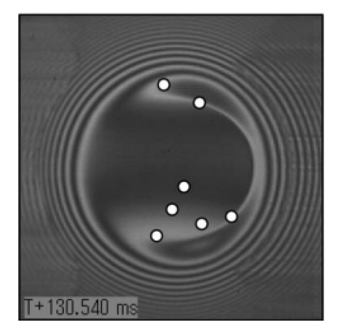
One other technological trend may also introduce additional importance to electrostatic discharge, the selection of lubricants. Traditionally, e-motor bearings have been greased for lifetime use but as e-motor speeds increase, in pursuit of higher efficiencies, forced oil lubrication is becoming more common. This is sometimes shared with the rotor cooling system. The demand for environmentally sustainable lubricant alternatives is also driving a growing market in water-based lubricants, many of which have the benefits of very low viscosity and good heat capacity but have quite different electrical conductivity [17].Capacitive bearing models have been created by Schneider et al. [18] among others. The tribological and electrical analysis of the bearing conjunction showed there is little effect of the EHL Petrusevich spike [19] and minimum film thickness portion of the hertzian region on the bearing capacitance. This finding is in agreement with a significant body of work which has used the capacitive properties of the Elasto-Hydrodynamic Lubrication (EHL) lubricant film as a method to measure its thickness, with the methodology being pioneered in the early 1960’s [20,21]. An experimental study conducted by Sunahara et al. [22] investigated the location of electrical discharge events within the hertzian contact patch. They used a modification of the interferometry technique pioneered by Gohar and Cameron [23] to capture the light emission produced during a discharge event. It was observed that the discharge locations were found in the highlighted regions shown in Figure 1.
The image shown in Figure 1 suggests that the location of discharge is associated with the regions of minimum film thickness, high-curvature, and high-pressure. In the region of interest discussed in Figure 1 it was Johns-Rahnejat and Gohar [24] and Safa and Gohar [25] who first managed to experimentally resolve the Petrusevich pressure spike in point and line contacts respectively. It has also been shown however that microscale surface roughness can, under certain conditions cause a significant effect on EHL film thickness and pressure distributions [26,27]. Venner and Napel [26] showed a significant flattening (amplitude reduction) of the microscale roughness in the EHL contact patch. The flattened asperities were accompanied by localised pressure spikes. Morales-Espejel [27] showed a complementary ripple amplitude model capable of accurately conforming to experimental micro EHL measurements. Experimental studies conducted by Becker and Abanteriba [2] on aircraft bearings proposed electrical discharge erosion took place between the asperities of the contiguous surfaces. At the same time there is an increased interest on the influence of lubricant physical properties on electrical discharge wear phenomena in rolling element bearings [28]. Despite the effect of amplitude reduction, it has been shown that the lambda ratio (oil film thickness over composite rms roughness) [29] plays an important role in predicting electrical discharge erosion wear in rolling element bearings [30].
A significant body of work has been conducted to determine lubricant electrical properties, experimental association between the lambda ratio and electrical discharge erosion wear. In addition, a significant amount of work has been conducted to predict surface roughness behaviour within elastohydrodynamic conjunctions, however, to date a numerical investigation of electrical field strength to indicate the location of discharge events in rough elastohydrodynamic contacts has not previously been published in open literature. This paper uses numerical analyses of infinite elastohydrodynamic line contacts and two-dimensional electrostatic problem to investigate if EHL microgeometry, lubricant density and microscale roughness has a significant influence on electrical field strength within dielectric lubricant films.
2. Methodology
To investigate the electrical field strength in elastohydrodynamic conjunctions a one-dimensional EHL model and two-dimensional electrostatic model are employed. The elastohydrodynamic problem is solved to determine the surface deflection, fluid film thickness and lubricant density. These properties are then passed as inputs to the electrostatic problem.
2.1. Contact Geometry and Mechanics
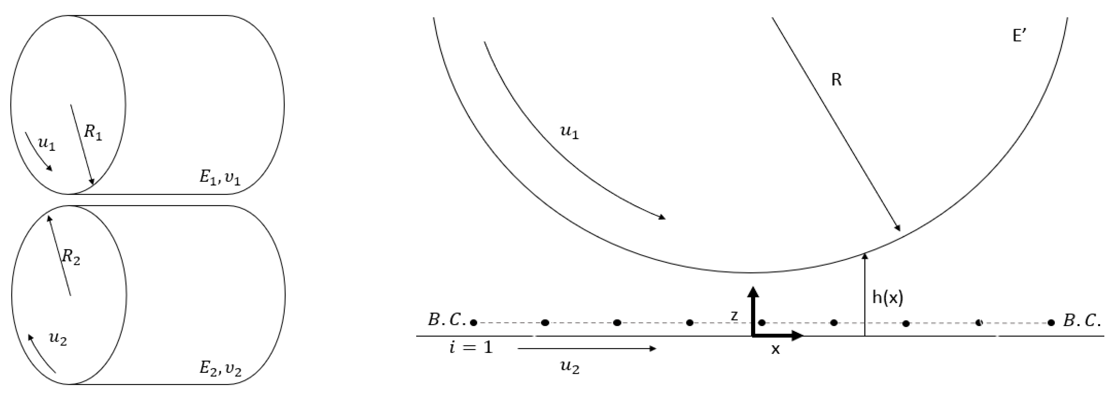
For simplicity an infinite line contact problem considering a pair of bodies which are axially aligned, cylindrical, counter formal and loaded against each other are considered. The two bodies rotate about their respective axes of cylindrical symmetry. The one-dimensional assumption is suitable for a range of conjunctions such as roller bearings and spur gears as a cross section at any axial position has the same tribological conditions (in the absence of misalignment, thermo-mechanical distortions and edge effects). A diagram representing the modeling approach is shown in Figure 2.
The dimensionless film thickness equation that describes the lubricant filled gap between the surfaces can be written as:
where is the surface roughness profile which is provided at the beginning of the results section. Due to the 2D model the roughness is in effect considered as infinitely wide ridges running perpendicular to the direction of entrainment. is an integration constant which is updated during the iterative load convergence scheme described in the solution procedure section. The third term describes the elastic deformation of the bodies resulting from the fluid film hydrodynamic pressure (P). While the last term describes the combined curvature of the two surfaces based on the dimensionless X coordinate. The surface roughness is considered as stationary as this study considers only pure rolling kinematics. Where the dimensionless X coordinate is defined as , where x is the coordinate and b is the hertzian contact half width:
where w is the dimensional load per unit length and E’ is the composite elastic modulus combining the elastic modulus (E) and Poisson’s ratio (υ) of the two bodies.
And R is the composite radius of curvature of the two surfaces in contact and can be written as:
The penultimate term in Equation (1) can be discretised as described by Venner and Napel [26] and the deflection kernel can be described as:
2.2. Hydrodynamics
A one-dimensional stationary form of Reynolds Equation (6) is discretised as described by Venner and Napel [26].
The dimensionless: Pressure P and Reynolds equation Coefficient ϵ terms are fully described in the Nomenclature and numerical values given in Table 1 and Table 2. The discretised form of the equation is given as:
where dX is the dimensionless grid spacing parameter and for convenience dimensionless terms are defined as: , and . A second order central difference of the Poiseuille term and first order upstream difference for the wedge term are employed to discretise the Reynolds equation as described by [26,33] due to the formulations improved stability [34]. The boundary conditions, labeled (B.C.) in Figure 2, are both set using dimensionless atmospheric pressure . The Moe’s dimensionless groups [35,36] are used to characterise the EHL contact.
where α is the pressure viscosity coefficient and us is the sum of the contacting surface velocities u1 and u2:
In this paper only pure rolling is consider and therefore u1 = u2. The load balance equation is written as:
2.3. Lubricant Physical Properties
The dielectric lubricant constant is dependent on the dimensionless lubricant density,, which varies with pressure as described by Dowson and Higginson [37]:
In the current study an isothermal assumption is employed and the dimensionless viscosity is described using Roelands [38] pressure viscosity relation as:
where z is Roelands pressure viscosity parameter, is a constant and α is the pressure viscosity index. There are limitations in the accuracy of Equation (13) to match experimentally measured data of real fluids [39,40]. In this study however where the specific lubricant is undefined the relation is deemed fit for purpose. In practice thermo-viscous behaviour and conjunctional thermal behaviour is often of importance and this would be an interesting addition to the current work [41].
For the electrostatic model the dielectric constant of the lubricant is required. The dielectric constant is calculated using the Clausius-Mossotti equation [18,42,43] using the dimensionless density calculated using Equation (12) which is determined during the elastohydrodynamic calculations.
where is the reference dielectric constant measured at the same temperature and pressure as the reference density [44].
2.4. Electrostatics
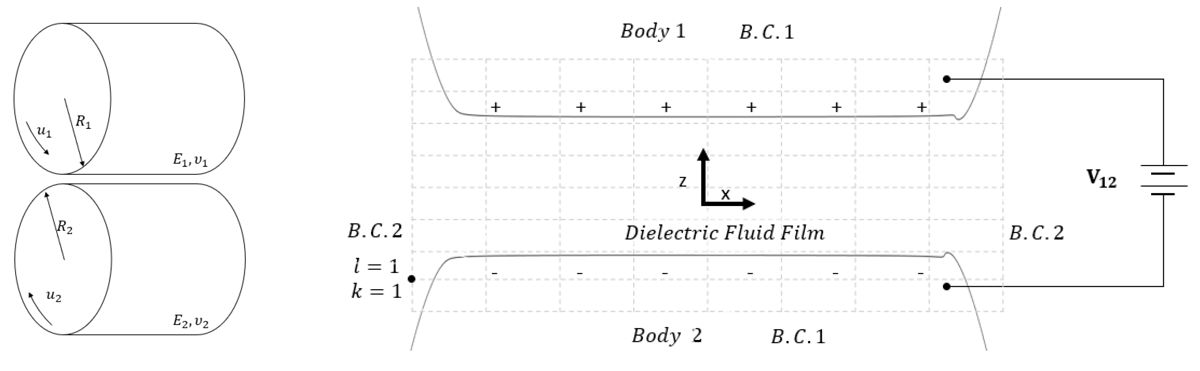
This paper investigates the electrical field intensity in an electrostatic condition during which the two electrically conductive contiguous surfaces are at a fixed potential of (±1V). These values were selected to be in the same order of magnitude as those observed in various applications [7,13,45,46] however the specific values have no other particular significance. The surface geometry is provided from the converged elastohydrodynamic model as shown in Figure 3.
The lubricant film which separates the surfaces is considered as a perfect dielectric which forms a continuous film between the surfaces. The effect of polar additive constituents of the lubricant (particularly detergents [47]), particulates [48] and other contaminants such as water are ignored in this analysis despite their potential importance when present in practice. The generalised Poisson equation shown below in Equation (15) describes the electrostatic behaviour of the elastohydrodynamic contact [49]:
where the charge density , dielectric constant ε and voltage potential V are functions of spatial position described by position vector r. The dielectric constant is calculated at each node from Equation (14) using the lubricant densities calculated during the elastohydrodynamic analysis. Finally, is the permittivity of free space and should not be confused with the dielectric constant . The two dimensional Poisson equation is necessary as from an electrostatic perspective it is not clear if the contact can be idealised as 1D as the curvature of the surfaces may have an effect on the field strength. The problem is 1D in terms of the EHL problem as the pressure is assumed constant across the thickness of the film and symmetric through the depth of the contact.
A successive over relaxed finite difference scheme is employed to solve the generalised Poisson equation in two dimensions. Although direct inversion is possible, the coefficient matrix is large and sparse making successive over relaxation preferable considering the computational resources available for this study. The dielectric constant is defined using a grid staggered from that of the voltage potential function as described by Nagel [50].
where the coefficients are described by Nagel [50] and are also provided for completeness in the Appendix A.
where is the residual and ξ is the damping factor. The field strength is found simply from the following definition. Typically, it is assumed the maximum electric field strength in an EHL contact is determined by the voltage potential across the contact and the minimum film thickness. The electrical field strength is therefore non-dimensionalised using the voltage potential ) between the two surfaces and minimum film thickness () as:
The model was constructed with the capability to use a refined grid spacing in comparison to the elastohydrodynamic model. To solve the electrostatic problem linear interpolation was used to transfer the lubricant density and surface geometry data between the two grids in the region −1.25< X <1.25. In addition, it was assumed the lubricant had a uniform density across the film at any X coordinate location. On the two conducting surfaces a Dirichlet boundary with fixed voltage potential is used, these form the top and bottom region of the solution domain. This boundary conditions are applied using the local charge, Q, in Equation (16). The local charge on bodies 1 and two is determined from the voltage potential as The solution domain is discretised and solved numerically using a successive over relaxation scheme.
2.5. Solution Procedure
The elastohydrodynamic problem is initialised using a hertzian pressure distribution and an initial guess for the integration constant. Then the hydrodynamic problem is solved values in the range −4 < X < 2, and the deflection field updated. A multigrid methodology outlined by Venner and Napel [26], Venner [33] and Wijnant [51] with the most refined grid consisting of 3200 nodes was employed. The refined grid has a sub micrometre spacing comparable to the surface roughness measurement lateral resolution. The integration constant is updated as:
where c is a numerical damping factor. Once the recursive multigrid solution has converged. The converged geometry and lubricant density are used to solve the electrostatic problem. The density of the lubricant from the elastohydrodynamic model is used to calculate the dielectric constant (Equation (14)) at each coordinate location. The electrostatic problem is initialised assuming a linearly varying voltage between the contiguous surfaces after which Equations (16) and (17) are solved until convergence is met.
3. Results
The lubricant physical properties and the key tribological properties are shown in Table 1 and Table 2 respectively. The values are chosen for purposes of validation and that they are typical of the tribological conditions found in many machine elements such as spur gear pairs and roller bearings. In addition, the minimum film thicknesses are sufficient that the quantum mechanical tunnel mechanism that leads to conductive behaviour in sub-nanometer thickness boundary films does not need to be considered [52,53]. For the electrostatic model it is considered , and .
3.1. Smooth Surface EHL and Electrical Field Strength Results
The elastohydrodynamic section of the model was validated against the data provided by Venner and Napel [26]. The predicted minimum and average film thicknesses for all conditions presented are within 3% of their published values as shown in Table 3. The results provide a good degree of confidence in the numerical elastohydrodynamic model for both minimum and average film thicknesses.
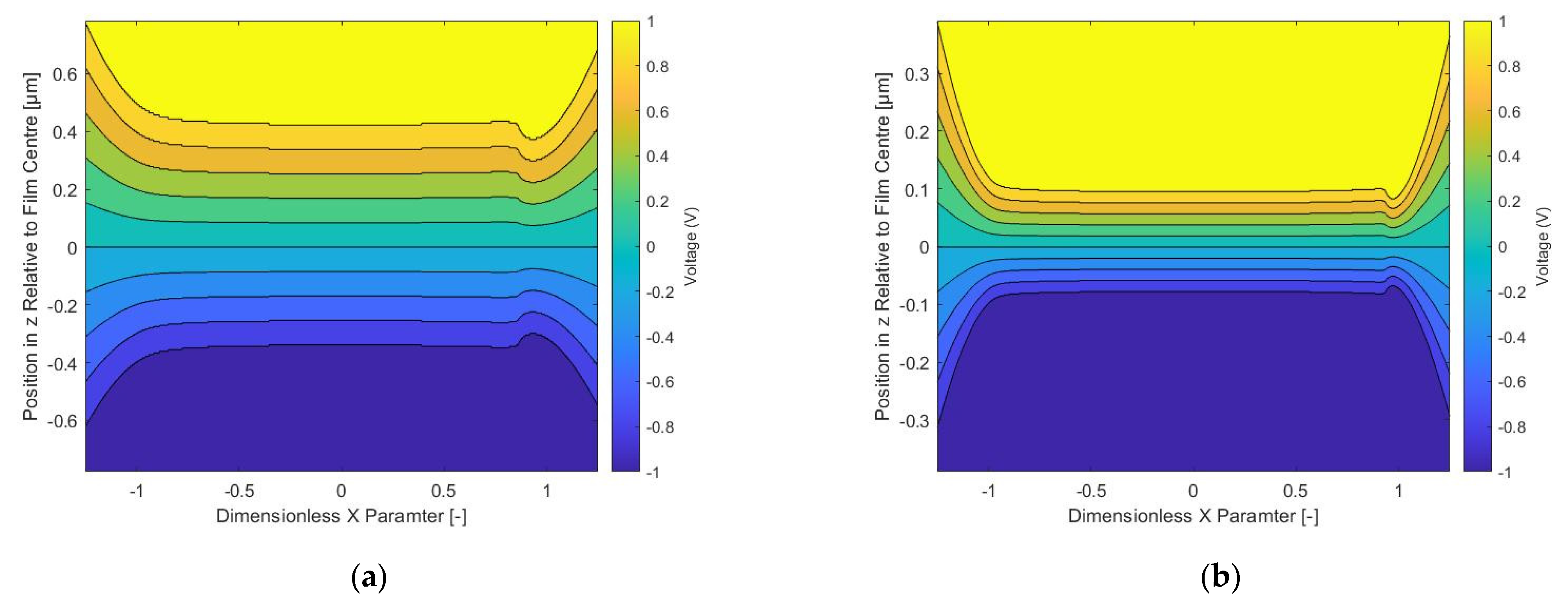
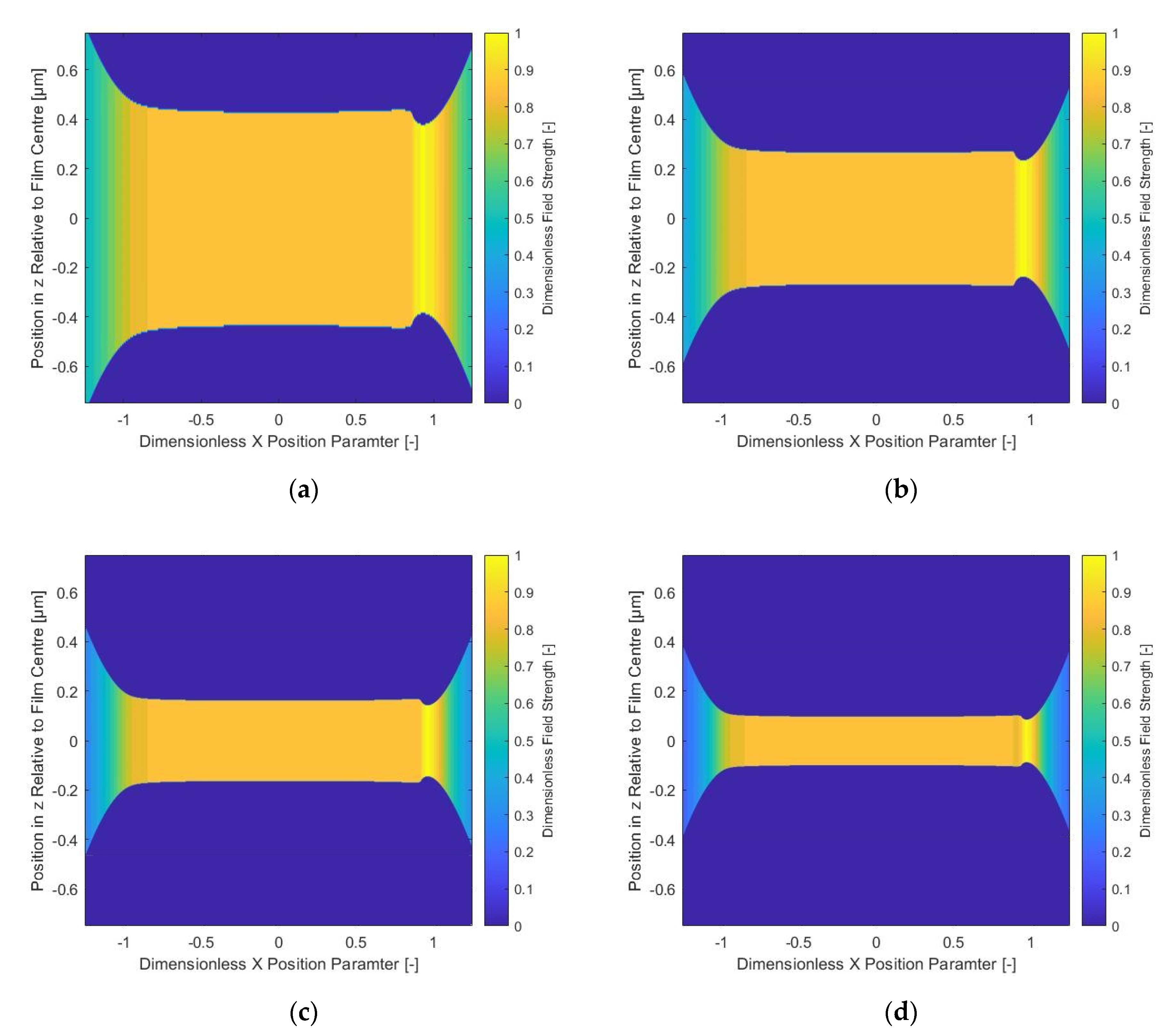
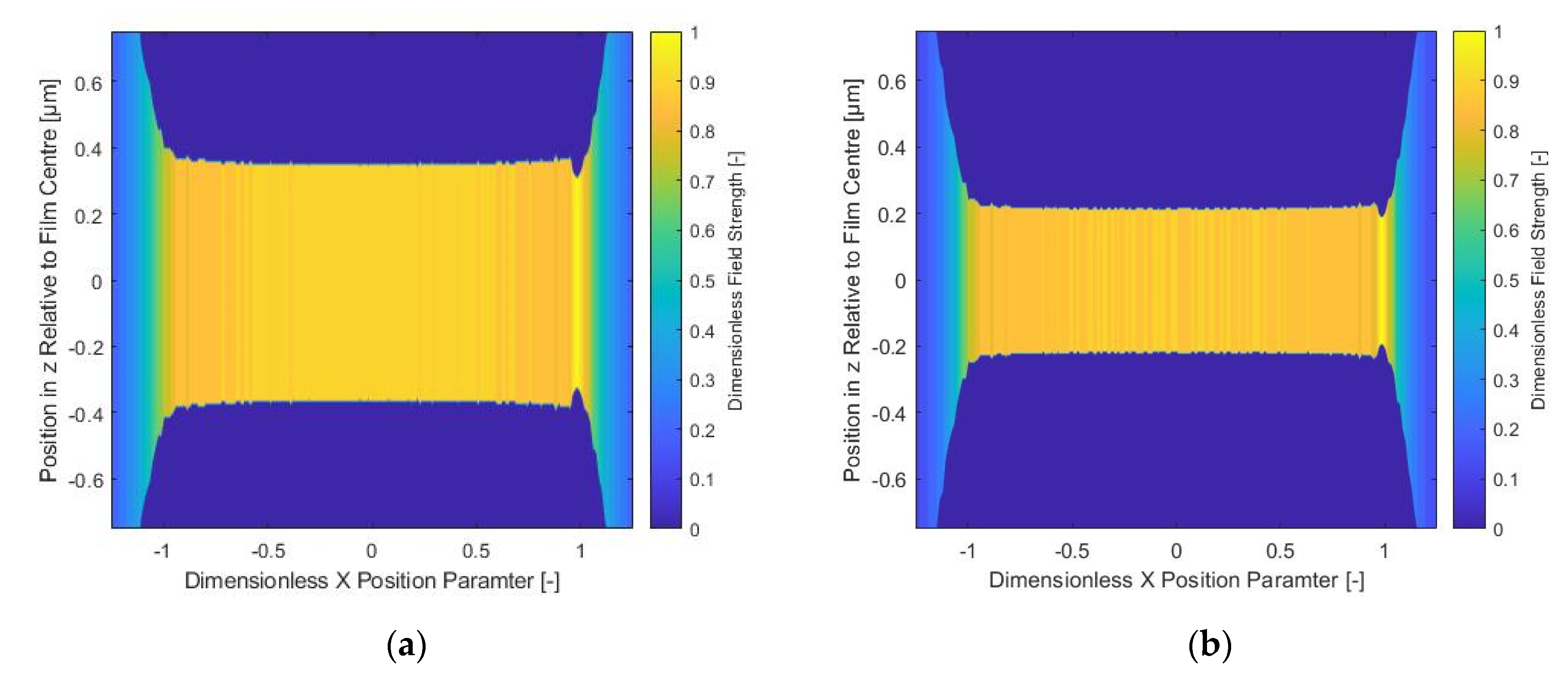
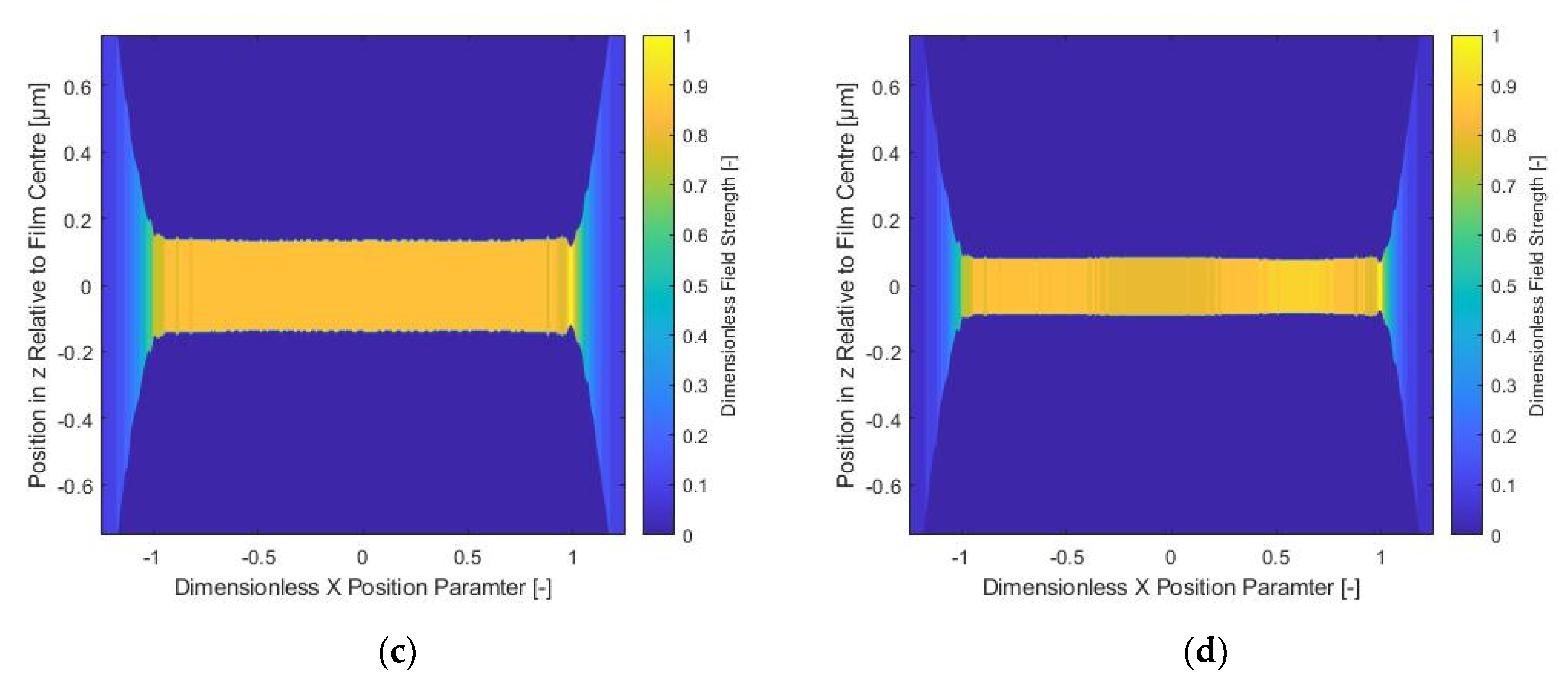
The voltage potential for two of the cases investigated is shown in Figure 4 where the constant voltage potential regions of ±1V are defined by the boundary condition applied to the conductive bodies. The electric field strength results for a range of M and L Moe’s non-dimensional EHL group values are presented for 1 and 2 GPa maximum hertzian contact pressure conjunctions shown in Figure 5 and Figure 6 respectively. The non-dimensional electric field strength is shown to have a maximum value of very close to unity at the location of the minimum film thickness. This is independent of the varying EHL behaviour characterised by the non-dimensional EHL groups. The electric field strength is therefore well predicted for a smooth conjunction by . The field strength in the central film thickness region is shown to consistently have a non-dimensional field strength value close to 0.9.
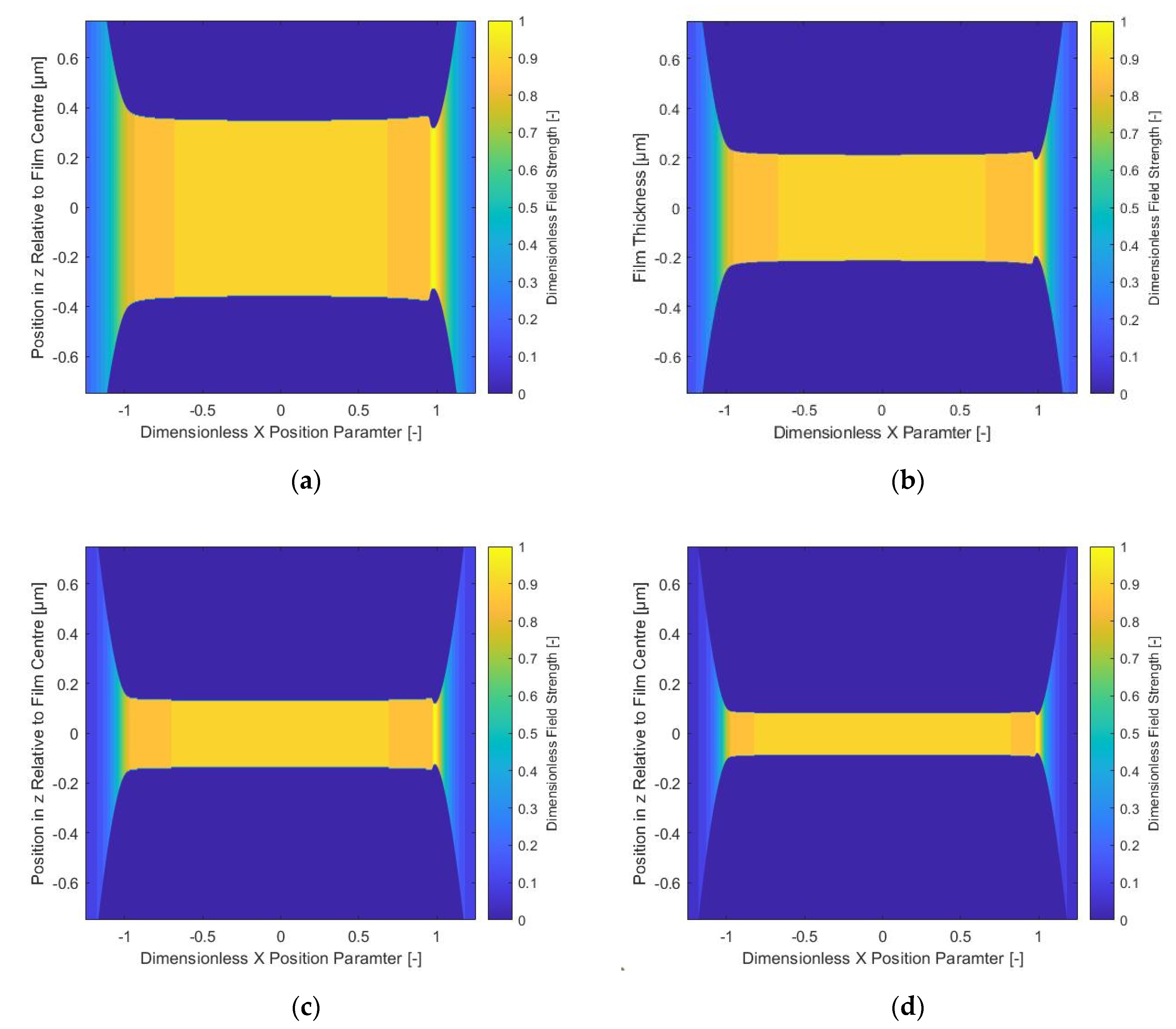
The results shown in Figure 6 show the same magnitude of dimensionless electrical field strength at the minimum and central film thickness regions even at the increased maximum contact pressure. This indicates a minor effect of the fluid film pressure induced change to its dielectric constant on the electrical field strength. Thermal effects resulting from flash temperature rise within the contact are ignored in this paper, however their significance on electrostatic behvaiour has not yet be evaluated. This provides an interesting further area of research.
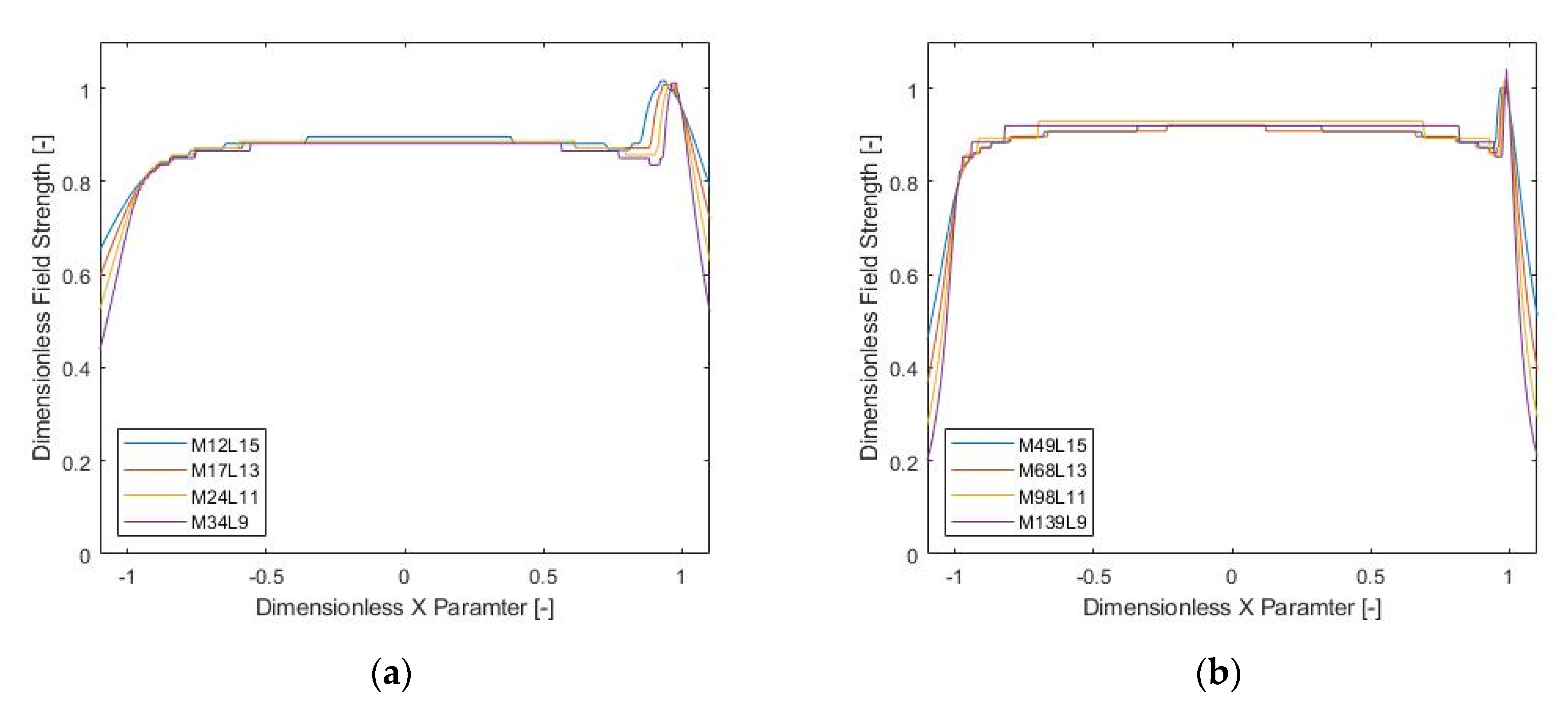
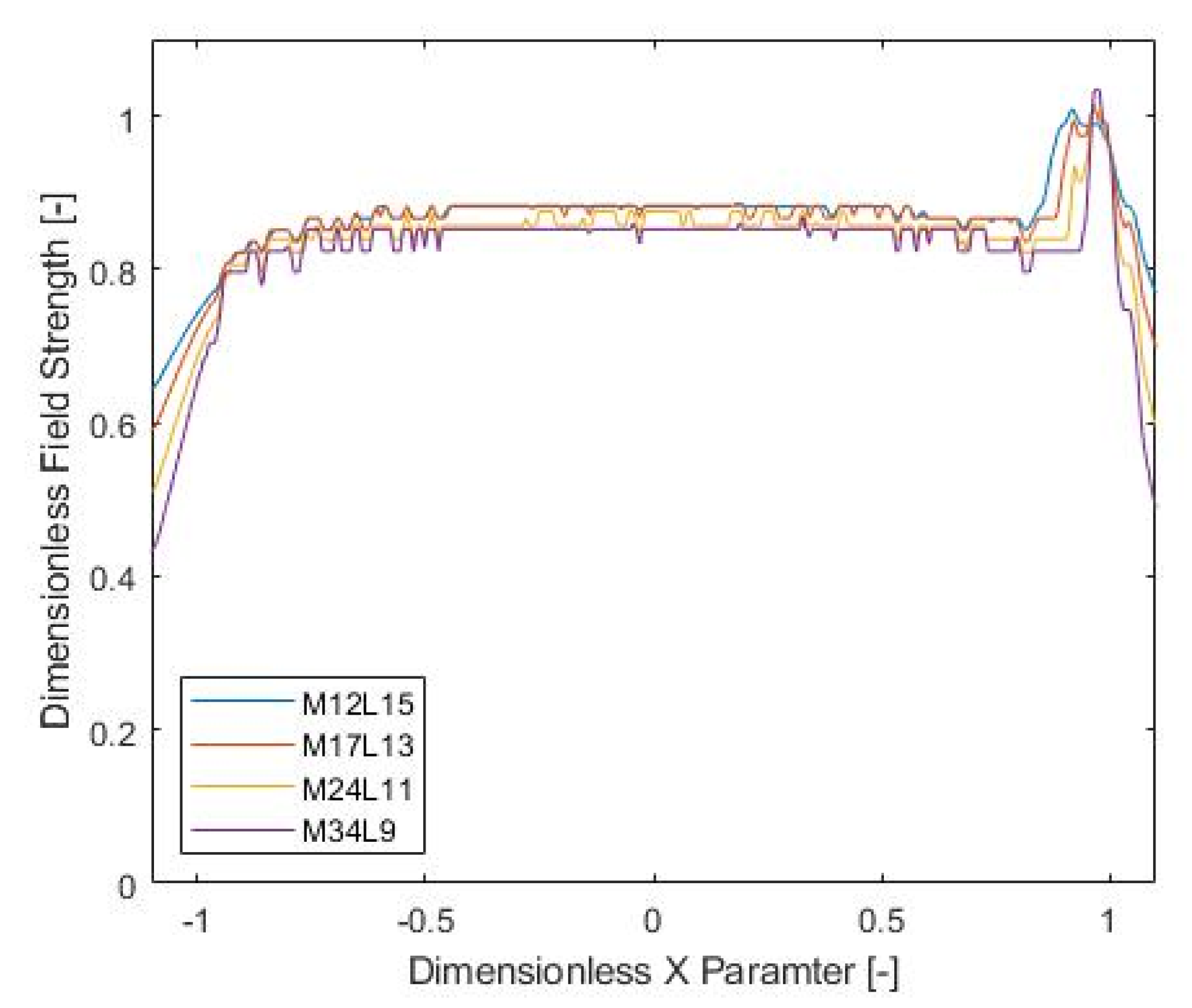
The electrical field strength clearly increases linearly with minimum film thickness. The cross section of electrical field strength at middle of the fluid film (as defined by half of the average film thickness) is presented in Figure 7. Interestingly, the width of the high field strength region located in the vicinity of the minimum film thickness location changes with M and L non-dimensional groups. The width of this region is of great interest to help determine the current density during electrical breakdown of the dielectric lubricant. Current density has been reported to be a key parameter to limit damage caused by electrical discharge erosion [54] with Busse et al. [45] suggesting the peak current density during a dielectric breakdown event should be less than 0.8 to not adversely affect bearing life. It is suggested that elastohydrodynamic micro geometry could have a role on the width of the breakdown region and therefore current density during discharge. The experimental research of Plazenet et al. [46] showed the maximum and average lateral dimension of pits formed through electrical discharge erosion are 4 µm and 1.7 µm diameter respectively. These dimensions are in the same order as the width of the minimum film thickness region rather than the hertzian contact half width for both the conjunctions in this research and for similar bearings in electric vehicle applications [55]. The presented numerical results therefore highlight the importance of elastohydrodynamic micro geometry on electrical discharge erosion wear behaviour.
3.2. Rough Surface EHL and Electrical Field Strength Results
A measured rough surface was included to investigate the effect of surface roughness on electrical field strength. A Mini-Traction-Machine disc commonly used for elastohydrodynamic experimentation was measured using a focus variation microscopy technique (Alicona InfiniteFocus G4) with ×100 magnification. The disc root mean square roughness Rq is 0.01 µm. The rough surface profile is shown in Figure 8.
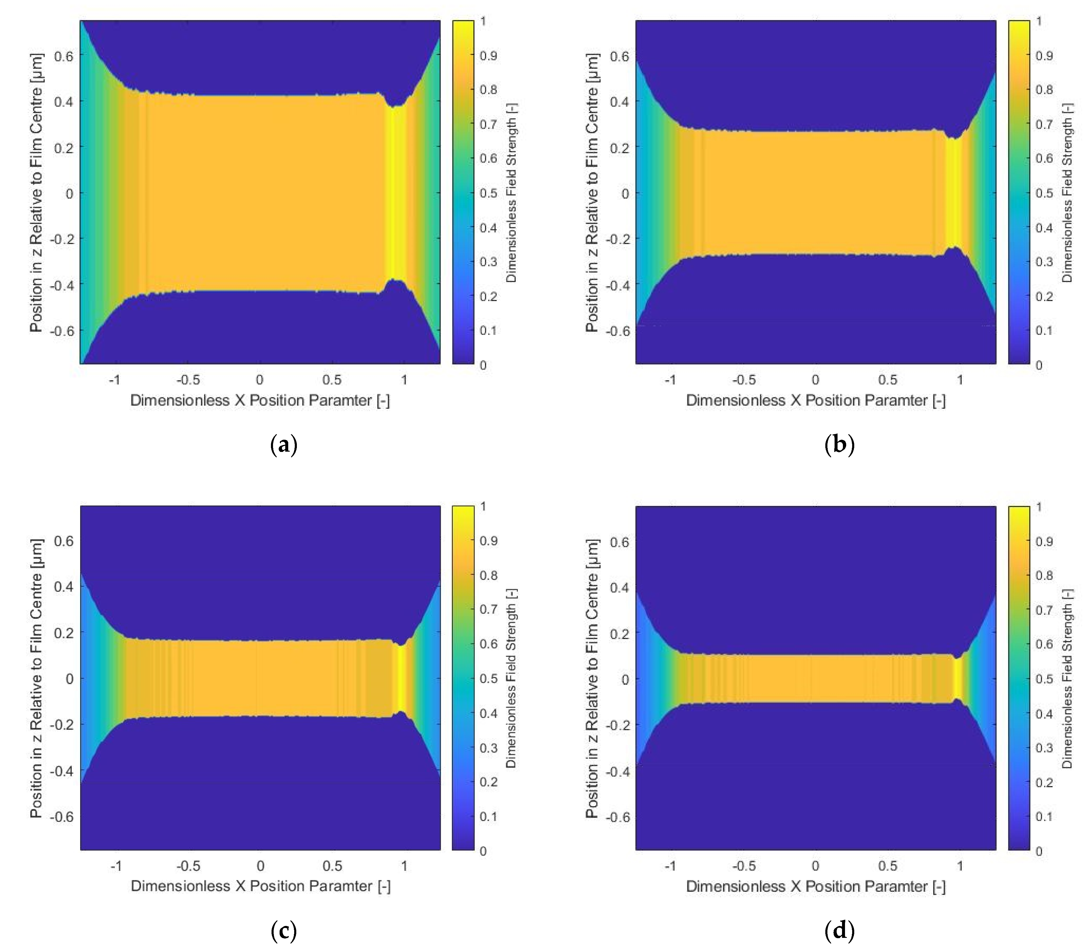
The roughness profile was included with in the elastohydrodynamic simulations and the converged solution provided to the electrostatic model. The roughness profile is truncated at ±0.05 µm to help stability of the EHL model. The results shown in Figure 9 and Figure 10 show the electrical field strength for the same conditions as previously investigated (1 and 2 GPa max hertzian contact pressure) but on this occasion with the inclusion of surface roughness.
The roughness is shown in Figure 9 and Figure 10 to create small perturbations to the electrical field strength due to a combination of small changes in local film thickness and pressure perturbations causing changes in the fluid film dielectric constant. The magnitude of the perturbations in dimensional electrical field strength are shown to be small relative to the electrical field strength at the location of the minimum film thickness in Figure 11.
4. Conclusions
The combined electrostatic and elastohydrodynamic numerical modelling approach expounded in this research has advanced the understanding of electrical field strength within elastohydrodynamic films. The model shows, for the first time, an approach to predicting the electrical field strength in elastohydrodynamic contacts. The key findings of this research are:
- For rough, full film, rolling EHL contacts amplitude reduction determines that can still be used to approximate the maximum electric field strength in the contact.
- Dimensionless Moe’s EHL group parameters (M and L) change the width of the high field strength region with implications for current density during arcing events.
- Changes in contact pressure and as result dielectric strength of the lubricant only have a minor effect on the non dimensional electrical field strength in the conjunction.
The findings of this paper will inform the tribological design of electro-mechanical systems and the lubricants and bearings that are required for their operation without the scourge of electrical discharge erosion.
Author Contributions
Conceptualization, M.L. and N.J.M.; Funding acquisition, M.L.; Investigation, S.A.M.; Methodology, N.J.M.; Software, S.A.M.; Supervision, M.L. and N.J.M.; Writing—original draft, N.J.M.; Writing—review & editing, S.A.M., M.L. and N.J.M. All authors have read and agreed to the published version of the manuscript.
Funding
This research received no external funding.
Acknowledgments
The authors would like to extend their thanks and appreciation to AVL List GmbH for the financial support and advice that has helped enabled this research.
Conflicts of Interest
The authors declare no conflict of interest.
Nomenclature
| Ampere | |
| Coefficients for Electrostatic calculations | |
| Density pressure relation coefficients | |
| Elastic modulus | |
| Dimensionless electric field strength | |
| Composite elastic modulus | |
| Minimum film thickness | |
| Film thickness | |
| Dimensionless film thickness | |
| Integration constant | |
| Grid index for elastohydrodynamic model in x direction | |
| Grid indexing for elastohydrodynamic model in x direction | |
| Grid index for electrostatic model in y direction | |
| Deflection kernel | |
| Grid index for electrostatic model in x direction | |
| Maximum hertzian pressure | |
| Roelands equation constant | |
| pressure | |
| Dimensionless pressure | |
| Local charge | |
| Position vector | |
| Dimensionless surface roughness | |
| sum of surface velocities | |
| Voltage potential | |
| Dielectric strength of fluid | |
| load per unit length | |
| coordinate | |
| Dimensionless coordinate | |
| z | Roelands pressure viscosity parameter |
| Pressure viscosity coefficient | |
| Voltage potential between surface 1 and surface 2 | |
| Reynold’s equation coefficient | |
| Permittivity of free space | |
| Dielectric constant at reference conditions | |
| Dielectric constant | |
| Electrical charge density | |
| dimensionless lubricant density | |
| velocity parameter | |
| viscosity at reference pressure and temperature | |
| Poisson’s ratio | |
| Numerical damping factor | |
| Subscript | |
| 1,2 denotes a property of Surface 1 and surface 2 respectively | |
Appendix A
References
- He, F.; Xie, G.; Luo, J. Electrical bearing failures in electric vehicles. Friction 2020, 8, 4–28. [Google Scholar] [CrossRef] [Green Version]
- Becker, A.; Abanteriba, S. Electric discharge damage in aircraft propulsion bearings. Proc. Inst. Mech. Eng. Part J J. Eng. Tribol. 2013, 228, 104–113. [Google Scholar] [CrossRef]
- Budinski, M.K. Failure analysis of a bearing in a helicopter turbine engine due to electrical discharge damage. Case Stud. Eng. Fail. Anal. 2014, 2, 127–137. [Google Scholar] [CrossRef] [Green Version]
- Symonds, N.; Corni, I.; Wood, R.; Wasenczuk, A.; Vincent, D. Observing early stage rail axle bearing damage. Eng. Fail. Anal. 2015, 56, 216–232. [Google Scholar] [CrossRef] [Green Version]
- Zhang, P.; Neti, P.; Salem, S. Electrical Discharge and Its Impact on Drivetrains of Wind Turbines. IEEE Trans. Ind. Appl. 2015, 51, 5352–5357. [Google Scholar] [CrossRef]
- Bialke, W. A discussion of friction anomaly signatures in response to electrical discharge in ball bearings. Aerosp. Mech. Symp. 2018, 44, 55–68. [Google Scholar]
- Prashad, H. Investigations of corrugated pattern on the surfaces of roller bearings operated under the influence of electrical fields. Lubr. Eng. 1988, 44, 710–717. [Google Scholar]
- ISO 15243:2017, Rolling Bearings—Damage and Failures—Terms, Characteristics and Causes, Int. Org. for Standardization, Standard. March 2017. Available online: https://www.iso.org/standard/59619.htmlBSIS15243:2017 (accessed on 2 April 2021).
- Prashad, H. Appearance of craters on track surface of rolling element bearings by spark erosion. Tribol. Int. 2001, 34, 39–47. [Google Scholar] [CrossRef]
- Joshi, A.; Blennow, J. Investigation of the static breakdown voltage of the lubricating film in a mechanical ball bearing. In Proceedings of the Nordic Insulation Symposium (No. 23), Trondheim, Norway, 9–12 June 2013. [Google Scholar]
- Beshev, D. Characterization of Electrical Lubricant Properties for Modelling of Electrical Drive Systems with Rolling Bearings; Forschungsvereinigung Antriebstechnik e.V. (FVA): Frankfurt, Germany, 2018; Available online: https://www.vdmashop.de/FVA/Bearing-World-Journal---Volume-2---December-2017-Print-1552.html (accessed on 20 April 2021).
- Chen, S.; Lipo, T.; Fitzgerald, D. Modeling of motor bearing currents in PWM inverter drives. IEEE Trans. Ind. Appl. 1996, 32, 1365–1370. [Google Scholar] [CrossRef] [Green Version]
- Erdman, J.; Kerkman, R.; Schlegel, D.; Skibinski, G. Effect of PWM inverters on AC motor bearing currents and shaft voltages. IEEE Trans. Ind. Appl. 1996, 32, 250–259. [Google Scholar] [CrossRef]
- Link, P.J. Minimizing electric bearing currents in ASD systems. IEEE Ind. Appl. Mag. 1999, 5, 55–66. [Google Scholar] [CrossRef]
- Benbouzid, M. Bibliography on induction motors faults detection and diagnosis. IEEE Trans. Energy Convers. 1999, 14, 1065–1074. [Google Scholar] [CrossRef]
- Thorsen, O.; Dalva, M. A survey of faults on induction motors in offshore oil industry, petrochemical industry, gas ter-minals, and oil refineries. IEEE Trans. Ind. Appl. 1995, 31, 1186–1196. Available online: http://0-www-scopus-com.brum.beds.ac.uk/inward/record.url?eid=2-s2.0-0029374064&partnerID=tZOtx3y1 (accessed on 1 December 2021). [CrossRef]
- Wijanarko, W.; Khanmohammadi, H.; Espallargas, N. Ionic Liquid Additives in Water-Based Lubricants for Bearing Steel—Effect of Electrical Conductivity and pH on Surface Chemistry, Friction and Wear. Front. Mech. Eng. 2022, 7, 756929. [Google Scholar] [CrossRef]
- Schneider, V.; Liu, H.-C.; Bader, N.; Furtmann, A.; Poll, G. Empirical formulae for the influence of real film thickness distribution on the capacitance of an EHL point contact and application to rolling bearings. Tribol. Int. 2021, 154, 106714. [Google Scholar] [CrossRef]
- Petrusevich, A.I. Fundamental conclusions from the contact-hydrodynamic theory of lubrication. Izv. Akad. Nauk. SSSR OTN 1951, 2, 209–223. [Google Scholar]
- Archard, J.F.; Kirk, M.T. Lubrication at point contacts. Proc. R. Soc. Lond. A 1961, 261, 532–550. [Google Scholar]
- Crook, A.W. The lubrication of rollers II. Film thickness with relation to viscosity and speed. Philos. Trans. R. Soc. Lond. Ser. A Math. Phys. Sci. 1961, 254, 223–236. [Google Scholar]
- Sunahara, K.; Ishida, Y.; Yamashita, S.; Yamamoto, M.; Nishikawa, H.; Matsuda, K.; Kaneta, M. Preliminary Measurements of Electrical Micropitting in Grease-Lubricated Point Contacts. Tribol. Trans. 2011, 54, 730–735. [Google Scholar] [CrossRef]
- Gohar, R.; Cameron, A. Optical Measurement of Oil Film Thickness under Elasto-hydrodynamic Lubrication. Nature 1963, 200, 458–459. [Google Scholar] [CrossRef]
- Johns-Rahnejat, P.M.; Gohar, R. Measuring contact pressure distributions under elastohydrodynamic point contacts. Tribotest 1994, 1, 33–53. [Google Scholar] [CrossRef]
- Safa, M.M.A.; Gohar, R. Pressure Distribution Under a Ball Impacting a Thin Lubricant Layer. J. Tribol. 1986, 108, 372–376. [Google Scholar] [CrossRef]
- Venner, C.H.; Napel, W.E.T. Surface Roughness Effects in an EHL Line Contact. J. Tribol. 1992, 114, 616–622. [Google Scholar] [CrossRef]
- Morales-Espejel, G.E.; Quiñonez, A.F. On the complementary function amplitude for film thickness in Mi-cro-EHL. Tribol. Int. 2019, 131, 631–636. [Google Scholar] [CrossRef]
- Gonda, A.; Capan, R.; Bechev, D.; Sauer, B. The Influence of Lubricant Conductivity on Bearing Currents in the Case of Rolling Bearing Greases. Lubricants 2019, 7, 108. [Google Scholar] [CrossRef] [Green Version]
- Tallian, T.E. On Competing Failure Modes in Rolling Contact. ASLE Trans. 1967, 10, 418–439. [Google Scholar] [CrossRef]
- Busse, D.F.; Erdman, J.M.; Kerkman, R.J.; Schlegel, D.W.; Skibinski, G.L. The effects of PWM voltage source inverters on the mechanical performance of rolling bearings. IEEE Trans. Ind. Appl. 1997, 33, 567–576. [Google Scholar] [CrossRef]
- Xu, K.; Chu, N.R.; Jackson, R.L. An investigation of the elastic cylindrical line contact equations for plane strain and stress considering friction. Proc. Inst. Mech. Eng. Part J J. Eng. Tribol. 2021. [Google Scholar] [CrossRef]
- Sharma, A.; Jackson, R.L. A Finite Element Study of an Elasto-Plastic Disk or Cylindrical Contact Against a Rigid Flat in Plane Stress with Bilinear Hardening. Tribol. Lett. 2017, 65, 112. [Google Scholar] [CrossRef]
- Venner, C.H. Multilevel Solution of the EHL Line and Point-Contact Problems. Ph.D. Thesis, University of Twente, Enschede, The Netherlands, December 1991. [Google Scholar]
- Lubrecht, A.A.; Breukink, G.A.C.; Moes, H.; Ten Napel, W.E.; Bosma, R. Solving Reynolds’ equation for EHL line contacts by application of a multigrid method. In Proceedings of the Thirteenth Leeds-Lyon Symposium on Tribology, Leeds, UK, 1 October 1987; pp. 175–182. [Google Scholar]
- Moes, H. Discussion on Paper D1 by D. Dowson. Proc. Inst. Mech. Eng. 1966, 180, 244–245. [Google Scholar]
- Moes, H. Communications. In Proceedings of the Symposium on Elastohydrodynamic Lubrication, London, UK, 21–23 September 1965; pp. 244–245. [Google Scholar]
- Dowson, D.; Higginson, G.R. Elasto-Hydrodynamic Lubrication: The Fundamentals of Roller and Gear Lubrication; Pergamon Press: Oxford, UK, 1966. [Google Scholar]
- Roelands, C.J.A. Correlational Aspects of the Viscosity Temperature-Pressure Relationship of Lubricating Oils. Ph.D. Thesis, Technische Hogeschool Delft, Delft, The Netherlands, 1966. [Google Scholar]
- Bair, S. High Pressure Rheology for Quantitative Elastohydrodynamics; Elsevier: Amsterdam, The Netherlands, 2019. [Google Scholar]
- Bair, S. Roelands’ missing data. Proc. Inst. Mech. Eng. Part J J. Eng. Tribol. 2004, 218, 57–60. [Google Scholar] [CrossRef]
- Liu, H.; Zhang, B.; Bader, N.; Poll, G.; Venner, C. Influences of solid and lubricant thermal conductivity on traction in an EHL circular contact. Tribol. Int. 2020, 146, 106059. [Google Scholar] [CrossRef]
- Bondi, A.A. Physical Chemistry of Lubricating Oils; Book Division, Reinhold Publishing Corporation: New York, NY, USA, 1951. [Google Scholar]
- Jackson, J.D. Classical Electrodynamics, 3rd ed.; Wiley: New York, NY, USA, 1999. [Google Scholar]
- Carey, A.A. The Dielectric Constant of Lubrication Oils; Computational Systems Inc.: Knoxville, TN, USA, 1998. [Google Scholar]
- Busse, D.; Erdman, J.; Kerkman, R.; Schlegel, D.; Skibinski, G. Bearing currents and their relationship to PWM drives. IEEE Trans. Power Electron. 1997, 12, 243–252. [Google Scholar] [CrossRef] [Green Version]
- Plazenet, T.; Boileau, T.; Caironi, C.C.; Nahid-Mobarakeh, B. Influencing Parameters on Discharge Bearing Currents in Inverter-Fed Induction Motors. IEEE Trans. Energy Convers. 2021, 36, 940–949. [Google Scholar] [CrossRef]
- McFadden, C.; Hughes, K.; Raser, L.; Newcomb, T. Electrical Conductivity of New and Used Automatic Transmission Fluids. SAE Int. J. Fuels Lubr. 2016, 9, 519–526. [Google Scholar] [CrossRef]
- Zhang, J.-G.; Mei, C.-H.; Wen, X.-M. Dust effects on various lubricated sliding contacts. In Proceedings of the Thirty Fifth Meeting of the IEEE Holm Conference on Electrical Contacts, Chicago, IL, USA, 18–20 September 1989; pp. 35–42. [Google Scholar]
- Sakidu, M.N.O. Numerical Techniques in Electromagnetics, 2nd ed.; CRC Press: Boca Raton, FL, USA, 2001. [Google Scholar]
- Nagel, J.R. Solving the Generalized Poisson Equation Using the Finite-Difference Method (FDM); Lecture Notes; Department of Electrical and Computer Engineering, University of Utah: Salt Lake City, UT, USA, 2011. [Google Scholar]
- Wijnant, Y.H. Contact Dynamics in the Field of Elastohydrodynamic Lubrication; Universiteit Twente: Enschede, The Netherlands, 2003. [Google Scholar]
- Holm, R. Electric Contacts, Theory and Applications, 4th ed.; Springer: Berlin/Heidelberg, Germany, 1967. [Google Scholar]
- Konchits, V.V.; Korotkevich, S.V.; Kim, C.K. Thermal effects and contact conductivity under boundary lubrication. Lubr. Sci. 2000, 12, 145–168. [Google Scholar] [CrossRef]
- Bell, S.; Cookson, T.J.; Cope, S.A.; Epperly, R.A.; Fischer, A.; Schlegel, D.W.; Skibinski, G.L. Experience with variable-frequency drives and motor bearing reliability. IEEE Trans. Ind. Appl. 2001, 37, 1438–1446. [Google Scholar] [CrossRef]
- Questa, H.; Mohammadpour, M.; Theodossiades, S.; Garner, C.; Bewsher, S.; Offner, G. Tribo-dynamic analysis of high-speed roller bearings for electrified vehicle powertrains. Tribol. Int. 2021, 154, 106675. [Google Scholar] [CrossRef]
Figure 1.
Location of discharge events shown by Sunahara et al. [22] in their paper “Preliminary measurements of electrical micropitting in grease-lubricated point contacts” in Tribology transactions, copyright © Society of Tribiologists and Lubrication Engineers, www.stle.org, reprinted by permission of Taylor & Francis Ltd. (Oxfordshire, UK), http://www.tandfonline.com (accessed on 20 January 2022) on behalf of Society of Tribiologists and Lubrication Engineers, www.stle.org.

Figure 2.
Depiction of elastohydrodynamic model formulation.

Figure 3.
Depiction of electrostatic model formulation.

Figure 4.
Electrical potneital of smooth surfaces EHL film at (a) M12L15 and (b) M34L9.

Figure 5.
Electrical field strength of smooth surface, 1 GPa max Hertzian contact pressure EHL contacts (a) M12L15 (b) M17L13 (c) M24 L11 (d) M34L9.
Figure 5.
Electrical field strength of smooth surface, 1 GPa max Hertzian contact pressure EHL contacts (a) M12L15 (b) M17L13 (c) M24 L11 (d) M34L9.

Figure 6.
Electrical field strength of smooth surface, 2 GPa max Hertzian contact pressure EHL contacts (a) M49 L15 (b) M68 L13 (c) M98 L11 (d) M139 L9.
Figure 6.
Electrical field strength of smooth surface, 2 GPa max Hertzian contact pressure EHL contacts (a) M49 L15 (b) M68 L13 (c) M98 L11 (d) M139 L9.

Figure 7.
Mid fluid film thickness electrical field strength in (a) 1GPa and (b) 2GPa max hertzian contact pressure conjunctions.
Figure 7.
Mid fluid film thickness electrical field strength in (a) 1GPa and (b) 2GPa max hertzian contact pressure conjunctions.

Figure 8.
(a) Measured rough surface profile and (b) example pressure distributions for M34L9 with and without roughness.
Figure 8.
(a) Measured rough surface profile and (b) example pressure distributions for M34L9 with and without roughness.

Figure 9.
Electrical field strength of rough surface 1 GPa max Hertzian contact pressure EHL contacts (a) M12L15 (b) M17L13 (c) M24 L11 (d) M34L9.
Figure 9.
Electrical field strength of rough surface 1 GPa max Hertzian contact pressure EHL contacts (a) M12L15 (b) M17L13 (c) M24 L11 (d) M34L9.

Figure 10.
Electrical field strength of rough surface 2 GPa max Hertzian contact pressure EHL contacts (a) M49L15 (b) M68L13 (c) M98 L11 (d) M139L9.
Figure 10.
Electrical field strength of rough surface 2 GPa max Hertzian contact pressure EHL contacts (a) M49L15 (b) M68L13 (c) M98 L11 (d) M139L9.


Figure 11.
Mid fluid film thickness dimensionless electrical field strength with roughness.


Table 1.
Lubricant physical properties.
| Parameter | Value | Units |
|---|---|---|
Table 2.
Geometric, Load, Elastic and Kinematic properties of the conjunction.
| Parameter | Value | Units |
|---|---|---|
| −4 to 2 | ||
Table 3.
Elastohydrodynamic model validation.
| 2GPa | Venner & Napel [26] | Current Model | ||||
|---|---|---|---|---|---|---|
| us [ms−1] | M | L | hmin [μm] | hav [μm] | hmin [μm] | hav [μm] |
| 8 | 49.2 | 15.7 | 0.65 | 0.73 | 0.64 | 0.71 |
| 4 | 69.6 | 13.2 | 0.39 | 0.44 | 0.38 | 0.43 |
| 2 | 98.4 | 11.1 | 0.24 | 0.27 | 0.24 | 0.26 |
| 1 | 139.1 | 9.35 | 0.15 | 0.17 | 0.15 | 0.16 |
Publisher’s Note: MDPI stays neutral with regard to jurisdictional claims in published maps and institutional affiliations. |
© 2022 by the authors. Licensee MDPI, Basel, Switzerland. This article is an open access article distributed under the terms and conditions of the Creative Commons Attribution (CC BY) license (https://creativecommons.org/licenses/by/4.0/).
Share and Cite
MDPI and ACS Style
Morris, S.A.; Leighton, M.; Morris, N.J. Electrical Field Strength in Rough Infinite Line Contact Elastohydrodynamic Conjunctions. Lubricants 2022, 10, 87. https://0-doi-org.brum.beds.ac.uk/10.3390/lubricants10050087
AMA Style
Morris SA, Leighton M, Morris NJ. Electrical Field Strength in Rough Infinite Line Contact Elastohydrodynamic Conjunctions. Lubricants. 2022; 10(5):87. https://0-doi-org.brum.beds.ac.uk/10.3390/lubricants10050087
Chicago/Turabian StyleMorris, Samuel A., Michael Leighton, and Nicholas J. Morris. 2022. "Electrical Field Strength in Rough Infinite Line Contact Elastohydrodynamic Conjunctions" Lubricants 10, no. 5: 87. https://0-doi-org.brum.beds.ac.uk/10.3390/lubricants10050087
Note that from the first issue of 2016, this journal uses article numbers instead of page numbers. See further details here.