A Novel Model for Evaluating the Operation Performance Status of Rolling Bearings Based on Hierarchical Maximum Entropy Bayesian Method


Abstract
:1. Introduction
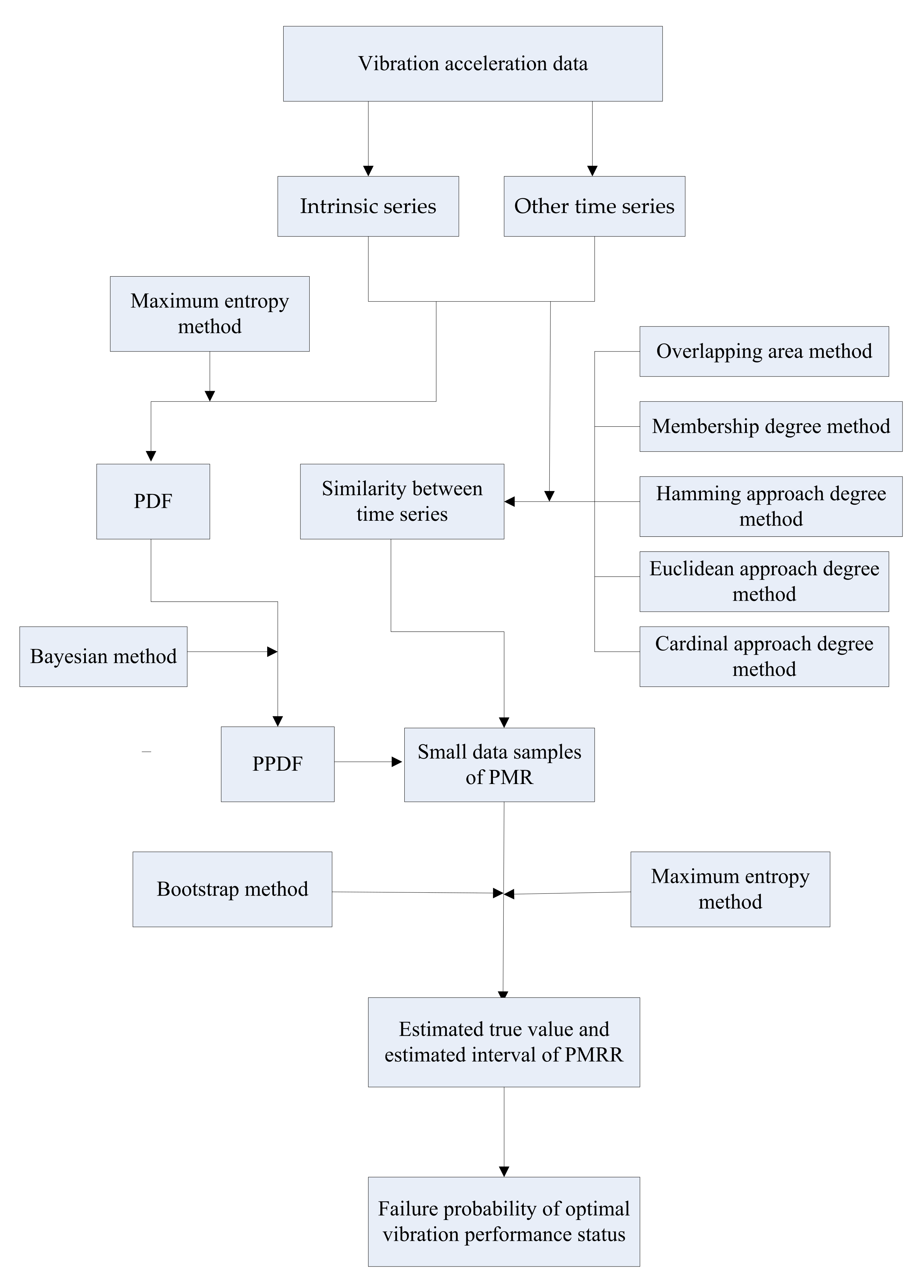
2. Mathematical Models
2.1. Solving PDF
2.2. Parameter Estimation
2.3. Calculating PPDF
2.4. Overlapping Area Method
2.5. Membership Degree Method
2.6. Approach Degree Method
2.7. Dynamic Evaluation of PMR
3. Experimental Verification
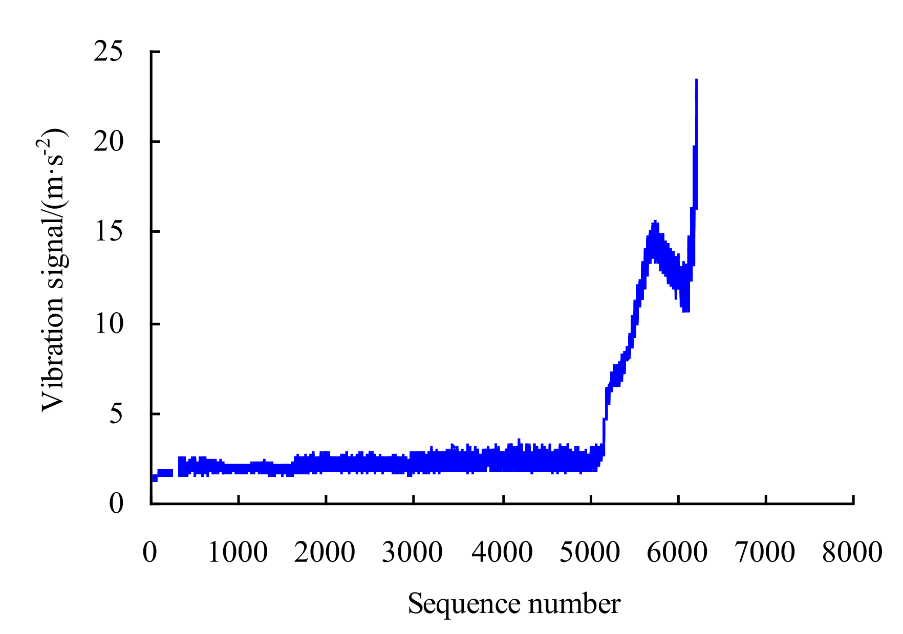
3.1. Case 1
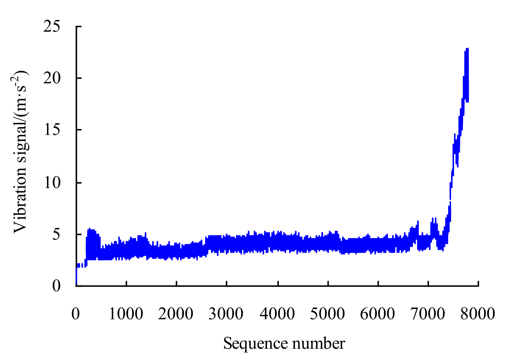
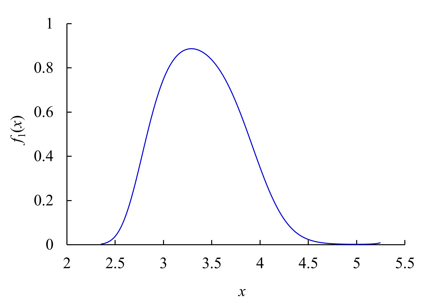
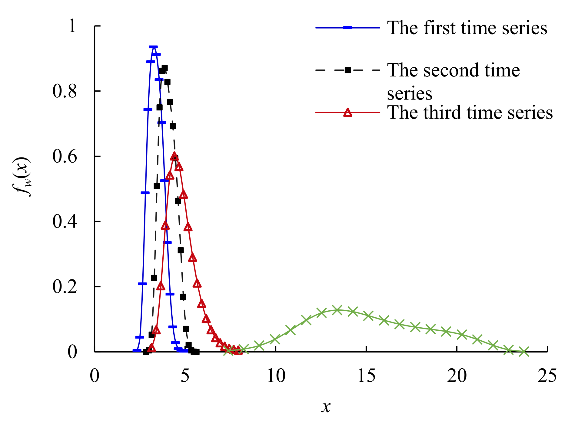
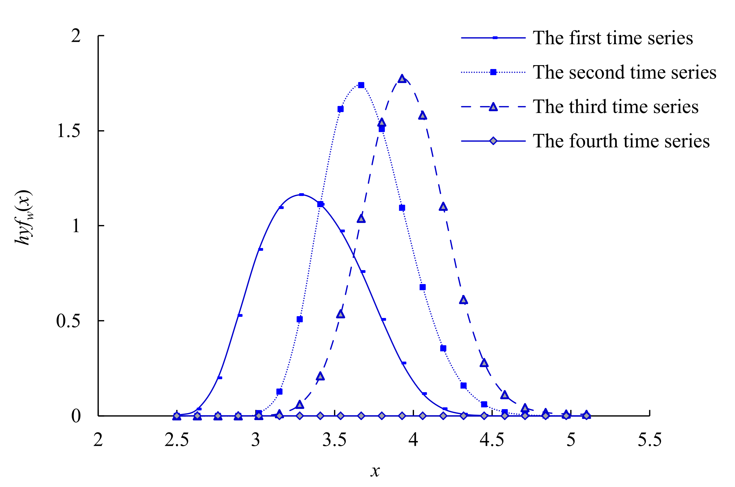
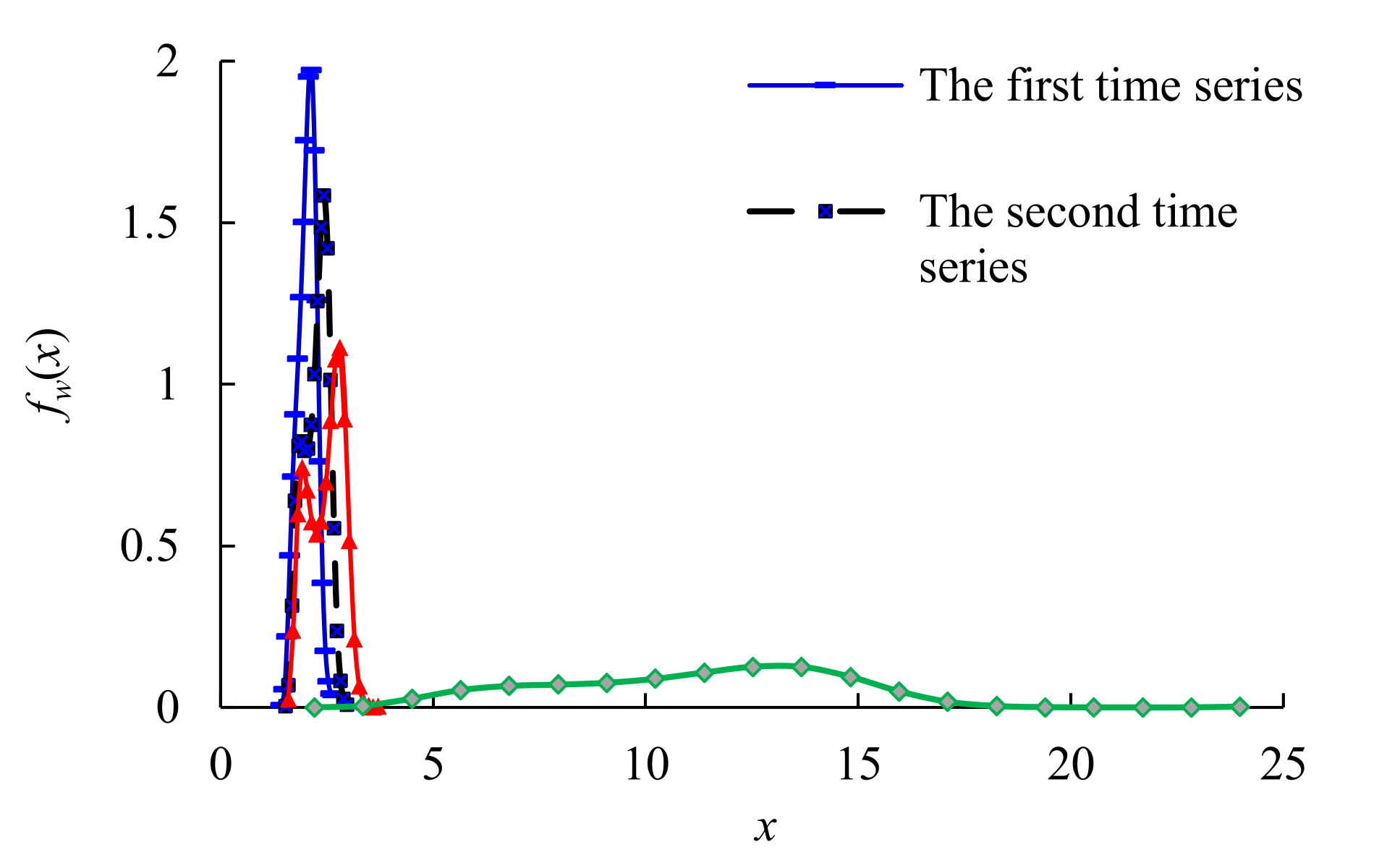
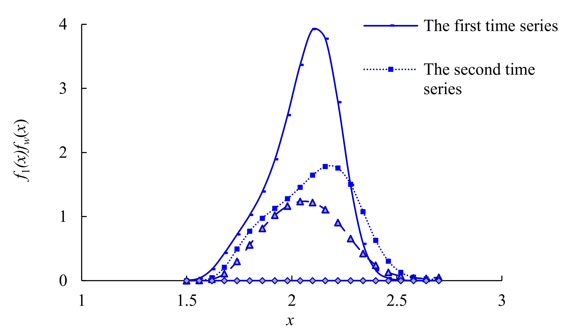
3.1.1. PDF of Data Samples of Time Series
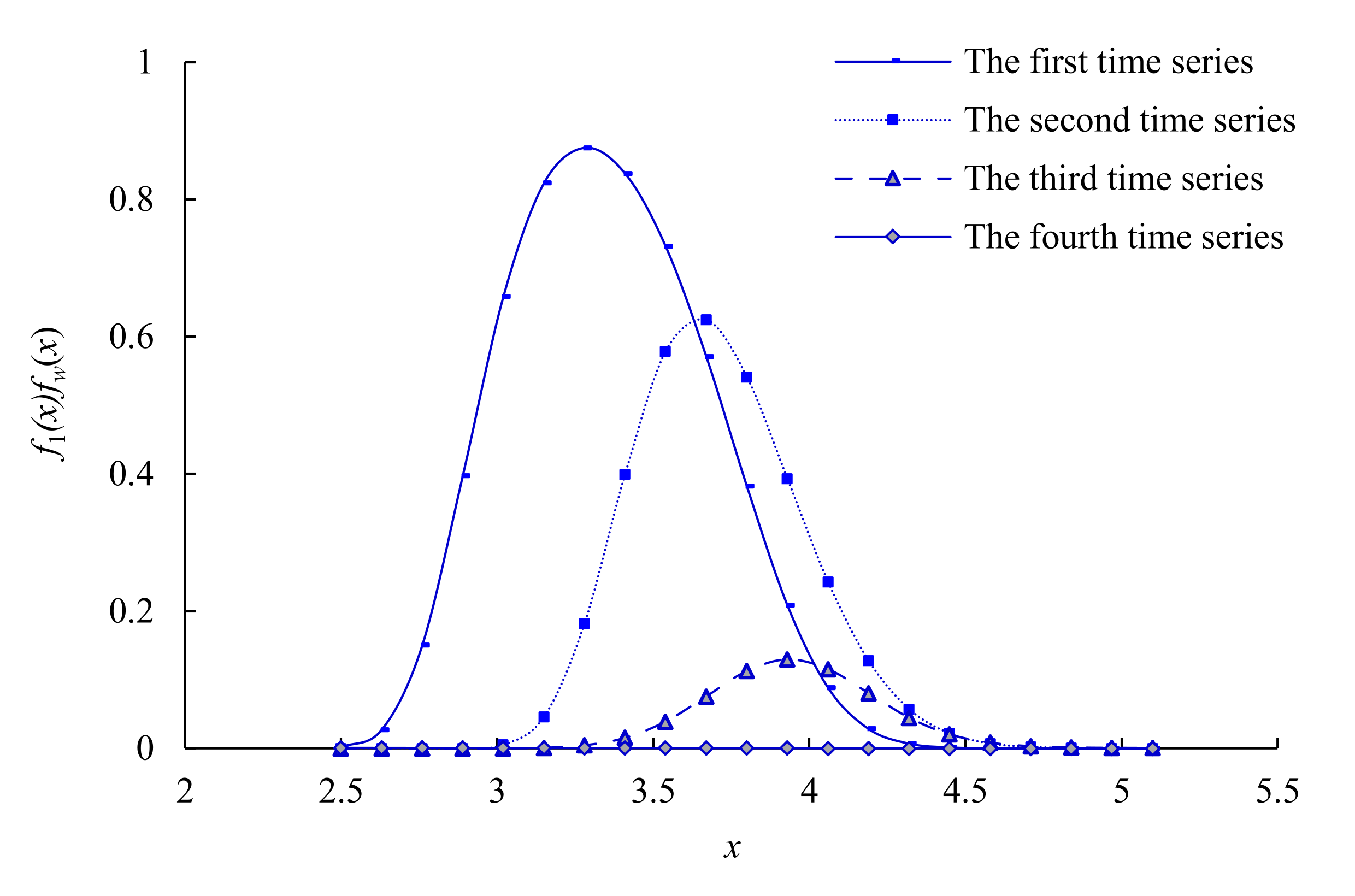
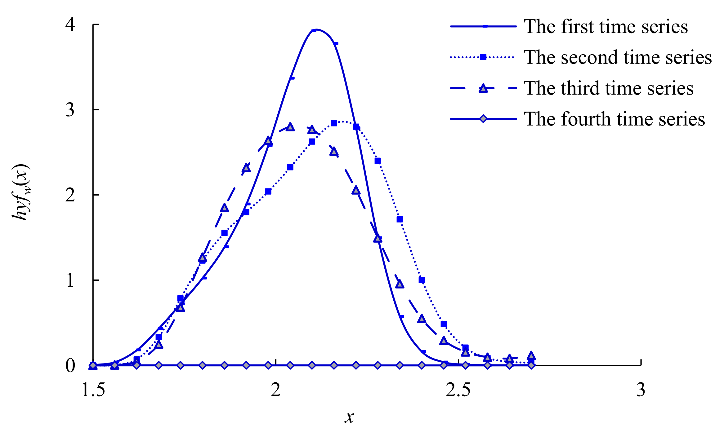
3.1.2. PPDF of Data Samples of Time Series
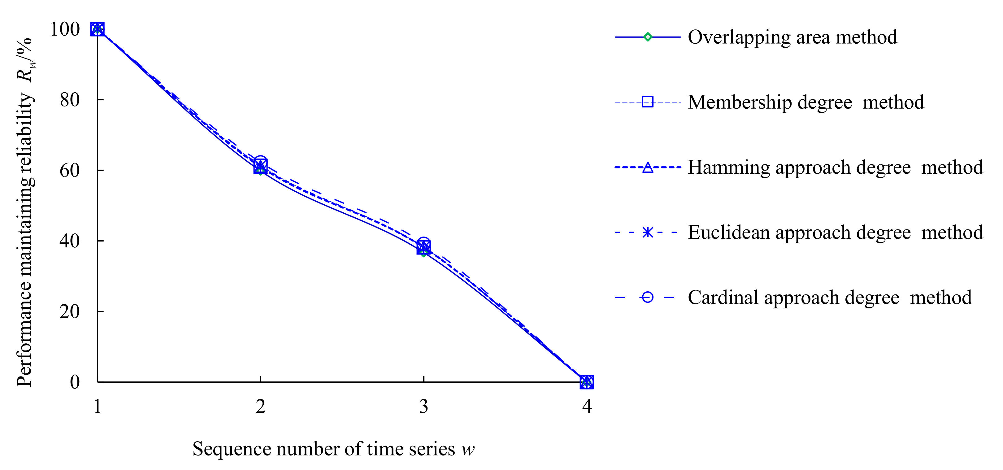
3.1.3. PMR of Time Series
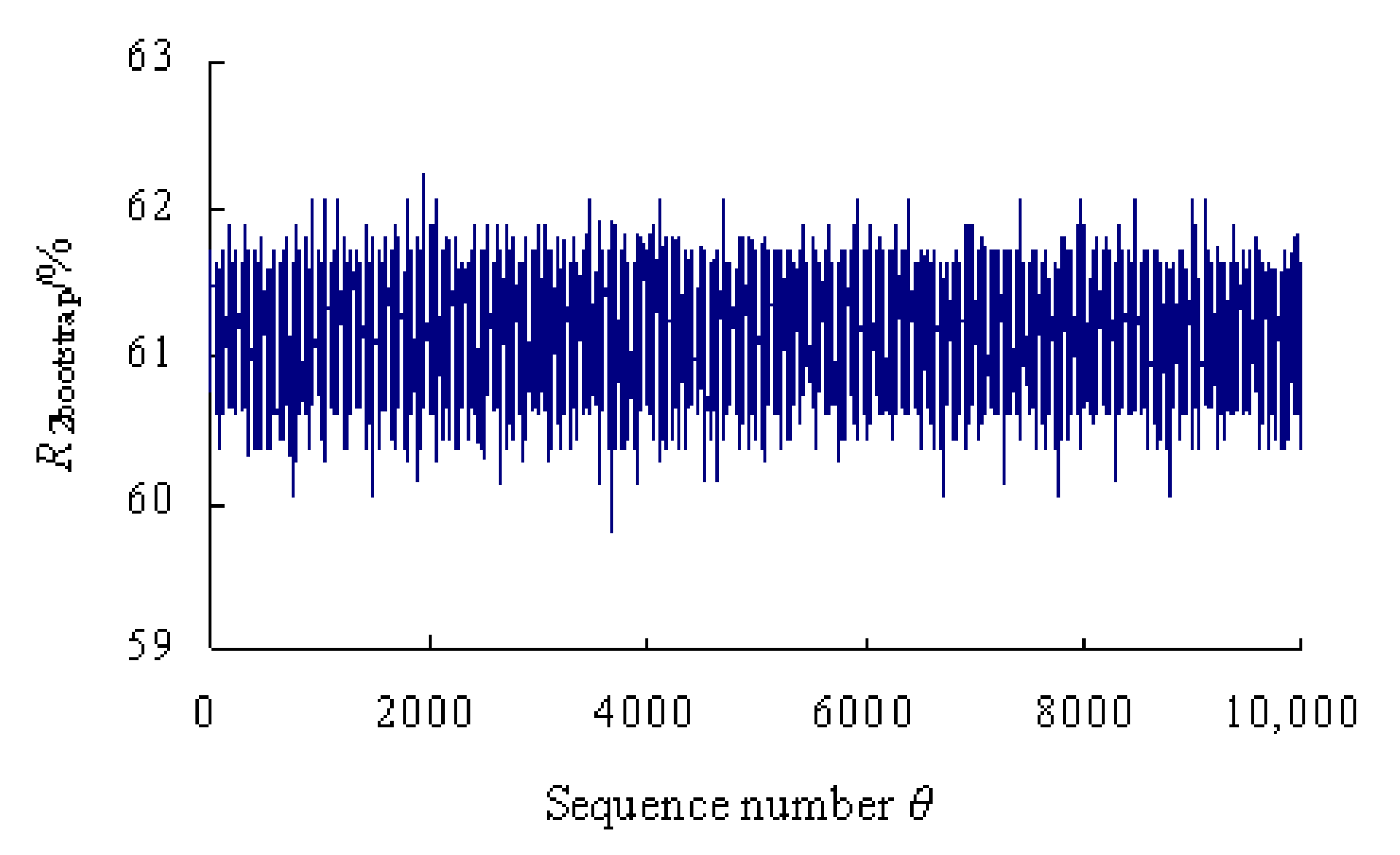
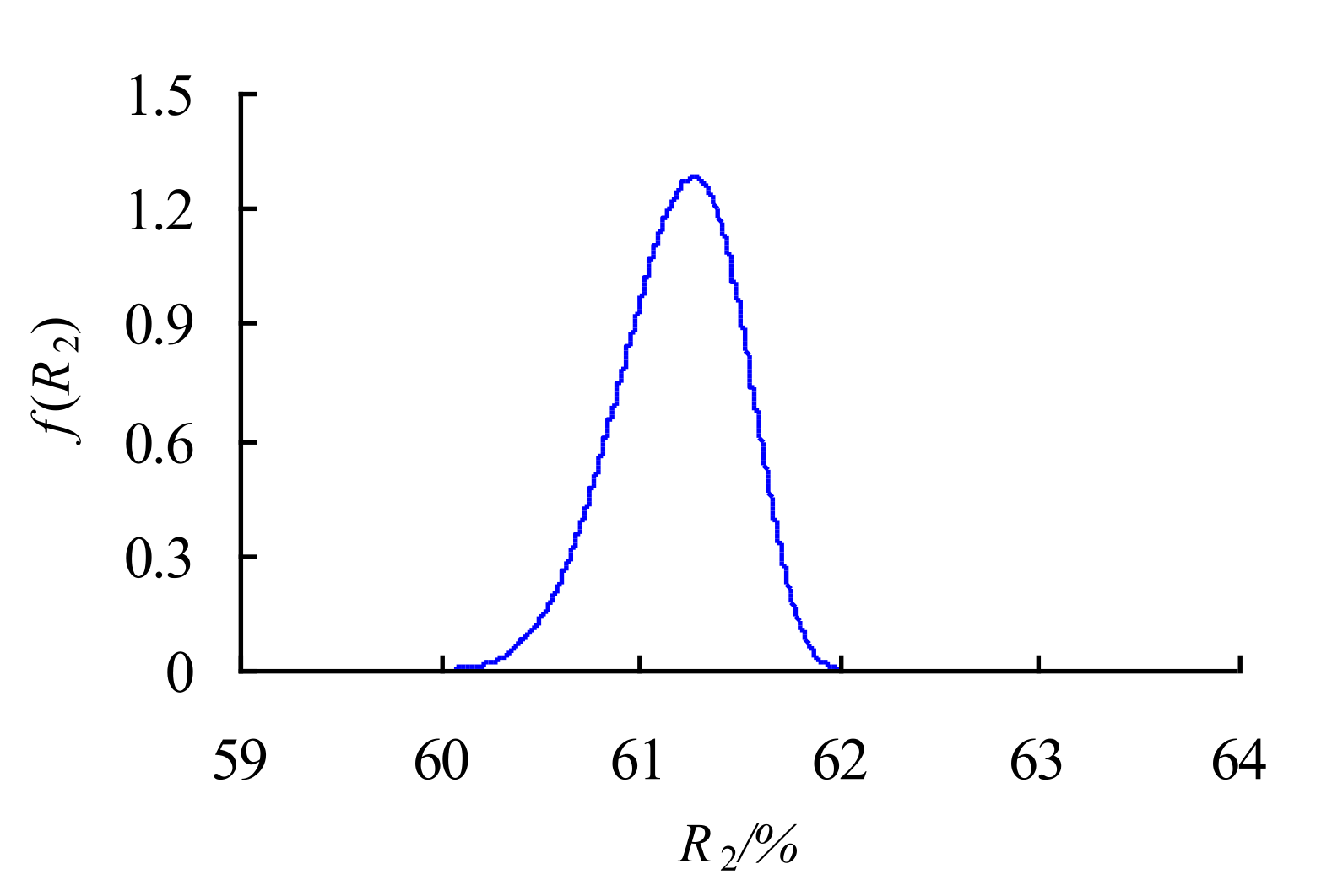
3.1.4. PMRR of Time Series
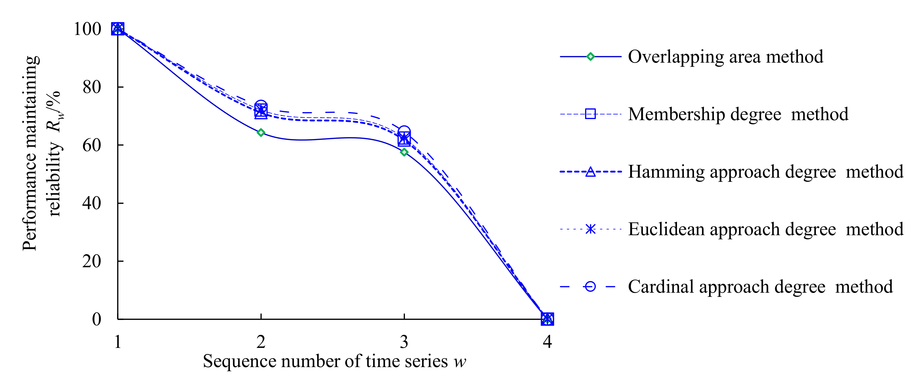
3.1.5. Fusion Results of Multiple Weighting Methods
3.2. Case 2
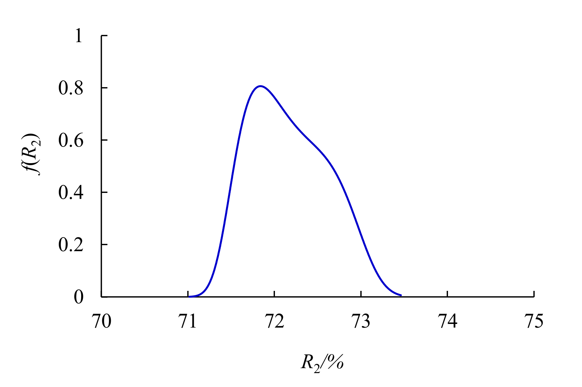
3.2.1. PDF of Data Samples of Time Series (Case 2)
3.2.2. PPDF of Data Samples of Time Series (Case 2)
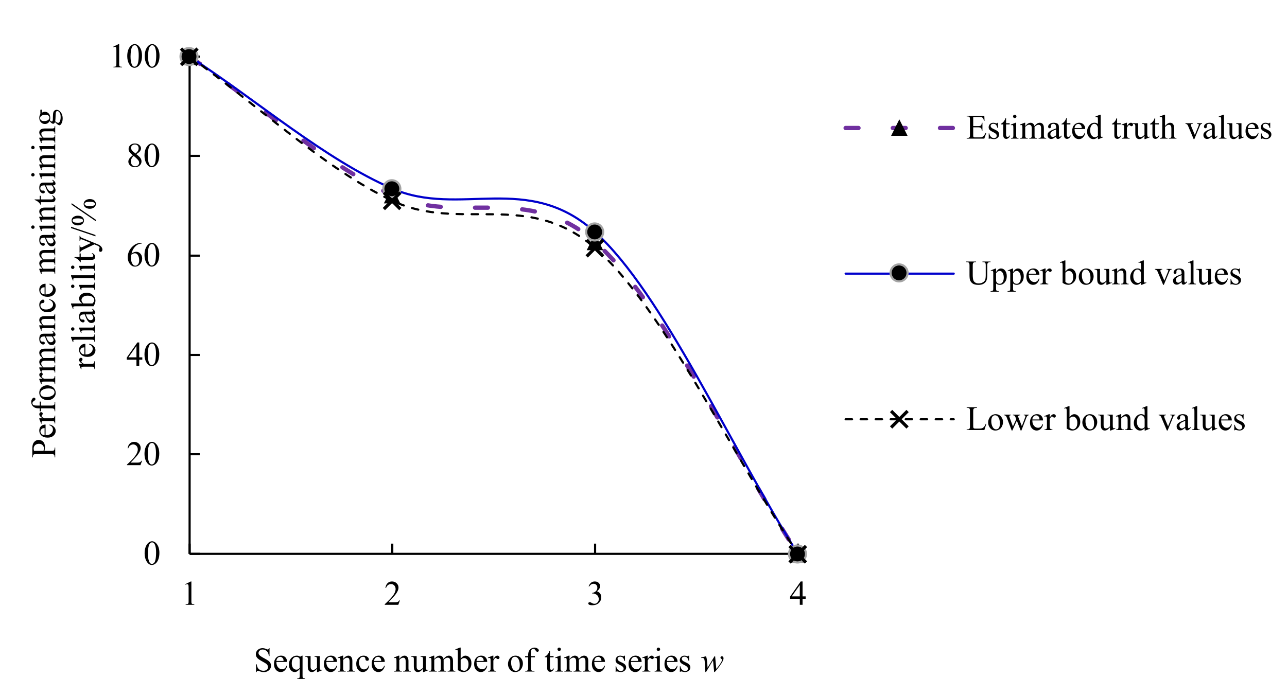
3.2.3. PMR of Time Series (Case 2)
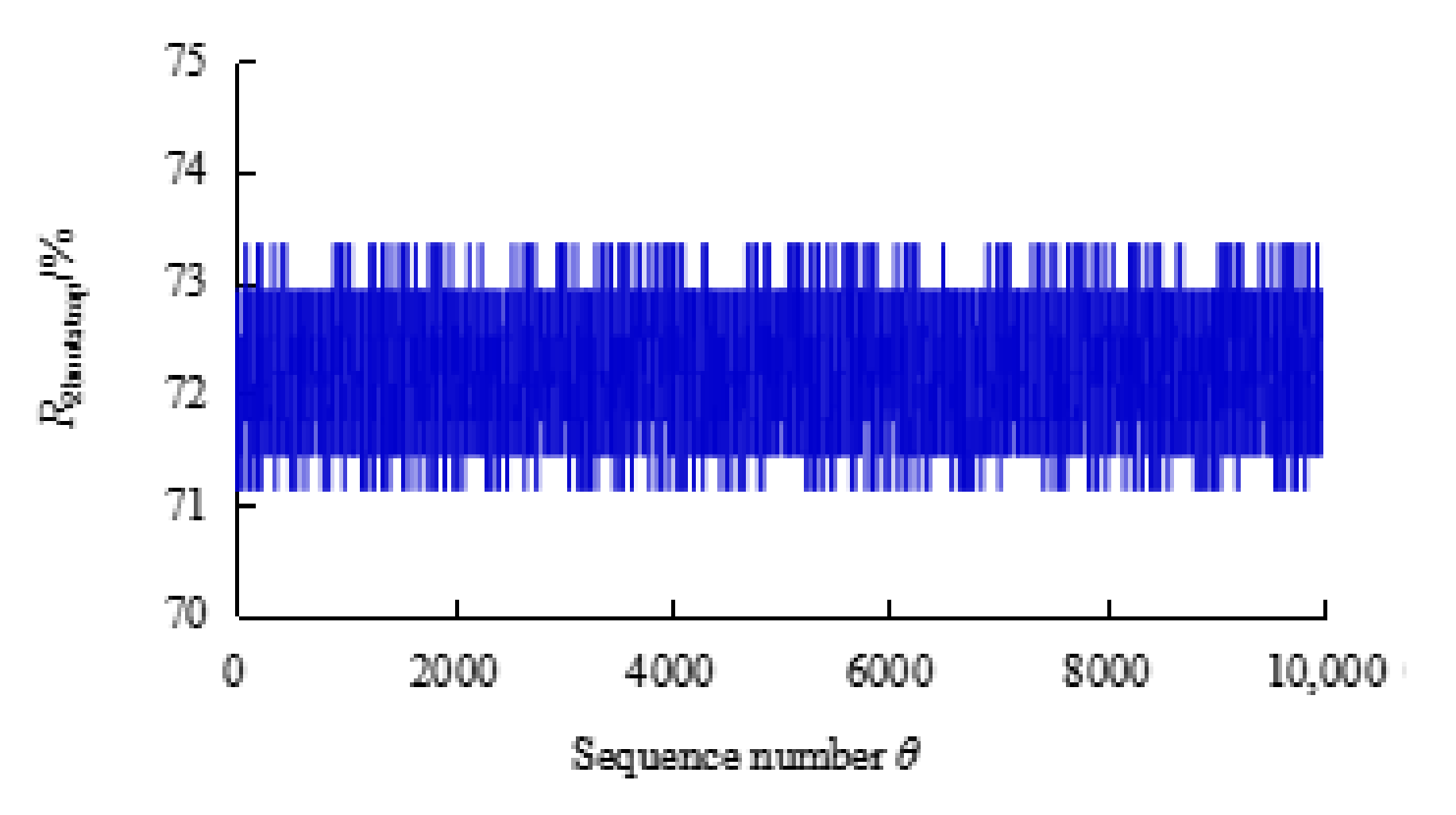
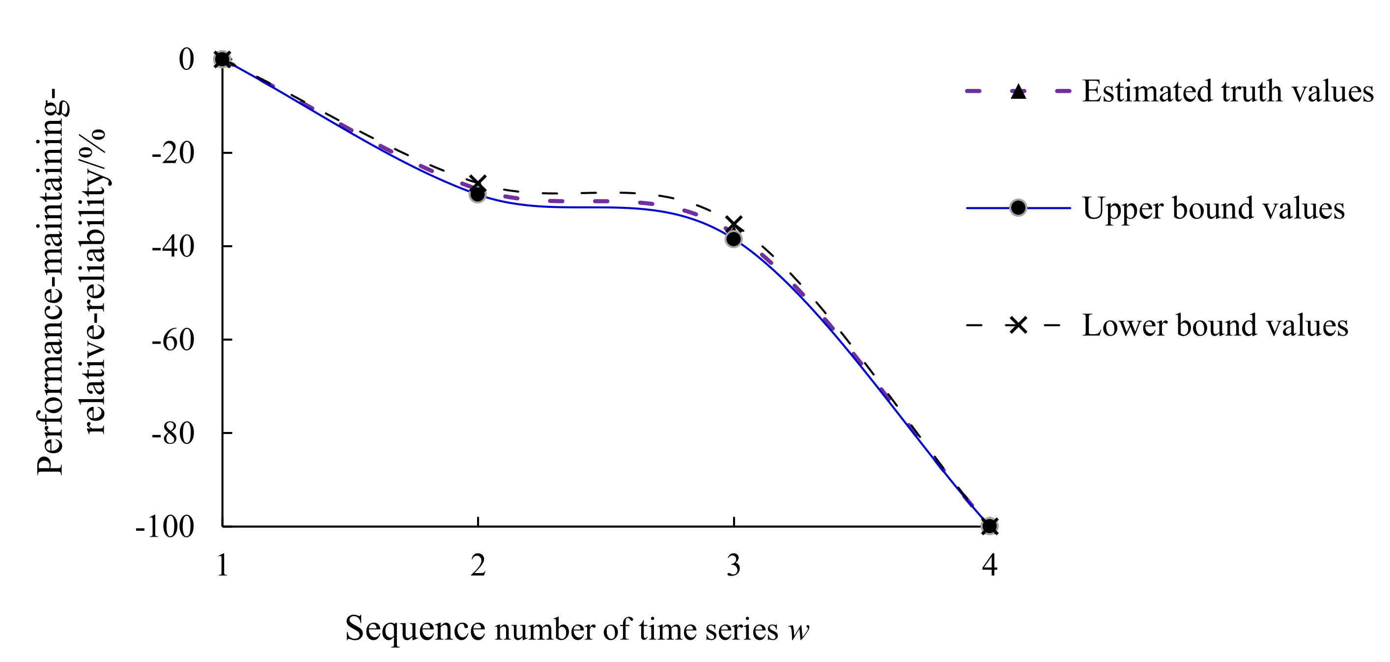
3.2.4. PMRR of Time Series (Case 2)
3.2.5. Fusion Results of Multiple Weighting Methods (Case 2)
4. Conclusions
- 1.
- Considering the operation status of rolling bearing, the variation degree of the optimal vibration performance status can be calculated more accurately to ensure effective maintenance of the system, reduce faults, and improve quality under the condition of traditional probability statistics.
- 2.
- The similarities between time series are obtained using the overlapping area method, membership degree method, Hamming approach degree method, Euclidean approach degree method, and cardinal approach degree method.
- 3.
- The maximum entropy method, Bayesian theory, and bootstrap method are fused fully to discover more information in time series of bearing vibration performance. The estimated true values and maximum entropy estimated intervals of PMR and PMRR are calculated to dynamically monitor the health status of rolling bearings online.
Author Contributions
Funding
Data Availability Statement
Conflicts of Interest
Nomenclature
| w | Order number of time series. |
| r | Number of time series. |
| N | Number of original data. |
| i | Order number of origin moment. |
| j | Highest order number of origin moment. |
| xw(k) | kth performance data in time series. |
| Xw | wth time series. |
| fw(x) | Probability density function of time series. |
| ciw | Lagrange multiplier. |
| Hw(x) | Information entropy of time series. |
| Ωw | Feasible domain for the data sample of time series. |
| lnfw(x) | Logarithmic value of fw(x). |
| miw | Order origin moment. |
| aw;bw | Mapping parameters. |
| hyfw(x) | PPDF of the wth time series Xw. |
| Ω1w | Intersection of feasible regions of data samples. |
| R1 | PMR of intrinsic series. |
| ηw | Overlapping area of PDF. |
| S1w | Overlapping area of PPDF. |
| dpk | Minkowski distance. |
| β3w | Cardinal approach degree. |
| xminw; xmaxw | Lower bound value and upper bound value in the time series. |
| xLw; xUw | Lower boundary value and upper boundary value of estimated interval. |
| x1L; x1U | Lower and upper bound values of confidence intervals for the PPDF of intrinsic series. |
| x*1L; x*1U | Lower and upper bound values of confidence intervals for the PDF of intrinsic series. |
| x1w; x2w | Abscissa values of the intersections for the PPDF of the wth time series and Intrinsic series. |
| x*1w; x*2w | Abscissa values of the intersections for the PDF of the wth time series and the intrinsic series. |
| Rw (1) | PMR calculated by using overlapping area method. |
| Rw (2) | PMR calculated by using membership degree method. |
| Rw (3) | PMR calculated by using Hamming approach degree method. |
| Rw (4) | PMR calculated by using Euclidean approach degree method. |
| Rw (5) | PMR calculated by using Cardinal approach degree method. |
| Rw | Data sample of PMR for the wth time series. |
| Rw(γ) | γth data in the PMR data sample for the wth time series. |
| Rwθ | θth bootstrap re-sampling sample. |
| B | Times of bootstrap re-sampling and number of bootstrap samples. |
| Rwθ(Θ) | Θth data in the θth bootstrap re-sampling sample of PMR |
| Rwbootstrap | Generated sample. |
| RwL; RwU | Lower-bound value and upper-bound value of PMR. |
| dw0; dwL; dwU | Estimated true value, lower-bound value, and upper-bound value of PMRR. |
| Probability density function. | |
| PMR | Performance maintaining reliability. |
| PMRR | Performance maintaining relative reliability. |
| PPDF | Posterior probability density function. |
| HMEBM | Hierarchical maximum entropy Bayesian method. |
References
- Wang, H.C.; Chen, J. Performance degradation assessment of rolling bearing based on bispectrum and support vector data description. J. Vib. Control. 2014, 13, 2032–2041. [Google Scholar] [CrossRef]
- Liu, J. A dynamic modelling method of a rotor-roller bearing-housing system with a localized fault including the additional excitation zone. J. Sound. Vib. 2020, 469, 115144. [Google Scholar] [CrossRef]
- Ma, S.; Zhang, X.; Yan, K.; Zhu, Y.; Hong, J. A study on bearing dynamic features under the condition of multiball-cage collision. Lubricants 2022, 10, 9. [Google Scholar] [CrossRef]
- Ai, Y.T.; Guan, J.Y.; Fei, C.W.; Tian, J.; Zhang, F.L. Fusion information entropy method of rolling bearing fault diagnosis based on n-dimensional characteristic parameter distance. Mech. Syst. Signal Pract. 2017, 88, 123–136. [Google Scholar] [CrossRef]
- He, Q.B.; Wu, E.H.; Pan, Y.Y. Multi-scale stochastic resonance spectrogram for fault diagnosis of rolling element bearings. J. Sound. Vib. 2018, 420, 174–184. [Google Scholar] [CrossRef]
- Moshrefzadeh, A.; Fasana, A. The autogram: An effective approach for selecting the optimal demodulation band in rolling element bearings diagnosis. Mech. Syst. Signal Pract. 2018, 105, 294–318. [Google Scholar] [CrossRef]
- Ye, L.; Xia, X.T.; Chang, Z. Dynamic prediction for accuracy maintaining reliability of superprecision rolling bearing in service. Shock. Vib. 2018, 2018, 7396293. [Google Scholar] [CrossRef]
- Zio, E. Reliability engineering: Old problems and new challenges. Reliab. Eng. Syst. Safe 2009, 94, 125–141. [Google Scholar] [CrossRef] [Green Version]
- Li, H.L.; Guo, C.H. Piecewise cloud approximation for time series mining. Knowl. Based Syst. 2011, 24, 492–500. [Google Scholar] [CrossRef]
- Xia, X.T.; Liu, B.; Li, Y.F.; Chen, X.; Zhu, W. Research on quality achieving reliability of bearing based on fuzzy weight. J. Aerosp. Power 2018, 33, 3013–3021. [Google Scholar]
- Bhaduri, M.; Zhan, J. Using empirical recurrence rates ratio for time series data similarity. IEEE Access 2018, 6, 30855–30864. [Google Scholar] [CrossRef]
- Shimizu, S. Weibull distribution function application to static strength and fatigue life of materials. Tribol. Trans. 2012, 55, 267–277. [Google Scholar] [CrossRef]
- Raje, N.; Sadeghi, F. Statistical numerical modelling of sub-surface initiated spalling in bearing contacts. Proc. Inst. Mech. Eng. Part J J. Eng. Tribol. 2009, 223, 849–858. [Google Scholar] [CrossRef]
- Zaretsky, E.V.; Branzai, E.V. Rolling bearing service life based on probable cause for removal-A tutorial. Tribol. Trans. 2017, 60, 300–312. [Google Scholar] [CrossRef]
- Zhang, N.; Wu, L.; Wang, Z.; Guan, Y. Bearing remaining useful life prediction based on naive Bayes and Weibull distributions. Entropy 2018, 20, 944. [Google Scholar] [CrossRef] [Green Version]
- Xia, X.T.; Lv, T.M. Dynamic prediction model for rolling bearing friction torque using grey bootstrap fusion method and chaos theory. Adv. Mater. Res. 2012, 443-444, 87–96. [Google Scholar] [CrossRef]
- Das, D.; Zhou, S.Y. Statistical process monitoring based on maximum entropy density approximation and level set principle. IIE Trans. 2015, 3, 215–229. [Google Scholar] [CrossRef]
- Chatterjee, A.; Mukherjee, S.; Kar, S. Poverty level of households: A multidimensional approach based on fuzzy mathematics. Fuzzy Inf. Eng. 2014, 4, 463–487. [Google Scholar] [CrossRef]
- Xia, X.T.; Lv, T.M.; Meng, F.N. Gray chaos evaluation model for prediction of rolling bearing friction torque. J. Test Eval. 2010, 38, 291–300. [Google Scholar]
- Xia, X.T. Reliability analysis of zero-failure data with poor information. Qual. Reliab. Eng. Int. 2012, 28, 981–990. [Google Scholar] [CrossRef]
- Xiao, W.; Cheng, W.; Zi, Y.; Zhao, C.; Sun, C.; Liu, Z.; Chen, J.; He, Z. Support evidence statistics for operation reliability assessment using running state information and its application to rolling bearing. Mech. Syst. Signal Pract. 2015, 60–61, 344–357. [Google Scholar] [CrossRef]
- Ghosh, S.; Polansky, A.M. Smoothed and iterated bootstrap confidence regions for parameter vectors. J. Multivar. Anal. 2014, 132, 171–182. [Google Scholar] [CrossRef]
- Wan, J.P.; Zhang, K.S.; Chen, H. The bootstrap and Bayesian bootstrap method in assessing bioequivalence. Chaos Solitons Fract. 2009, 41, 2246–2249. [Google Scholar]
- Wang, Y.; Zhou, W.; Dong, D.; Wang, Z. Estimation of random vibration signals with small samples using bootstrap maximum entropy method. Measurement 2017, 105, 45–55. [Google Scholar] [CrossRef]
- Chang, J.Y.; Hall, P. Double-bootstrap methods that use a single double-bootstrap simulation. Biometrika 2015, 102, 203–214. [Google Scholar] [CrossRef] [Green Version]
- Wu, F.X.; Wen, W.D. Scatter factor confidence interval estimate of least square maximum entropy quantile function for small samples. Chin. J. Aeronaut. 2016, 29, 1285–1293. [Google Scholar] [CrossRef] [Green Version]
- Edwin, A.B.; Angel, K.M. A clustering method based on the maximum entropy principle. Entropy 2015, 1, 151–180. [Google Scholar]
- Kwon, Y. Design of Bayesian zero-failure reliability demonstration test for products with Weibull lifetime distribution. J. Appl. Reliab. 2014, 14, 220–224. [Google Scholar]
- Jha, D.K.; Virani, N.; Reimann, J.; Srivastav, A.; Ray, A. Symbolic analysis-based reduced order Markov modeling of time series data. Signal Process 2018, 149, 68–81. [Google Scholar] [CrossRef] [Green Version]
- Xiao, N.C.; Li, Y.F.; Wang, Z.; Peng, W.; Huang, H.Z. Bayesian reliability estimation for deteriorating systems with limited samples using the maximum entropy approach. Entropy 2013, 12, 5492–5509. [Google Scholar] [CrossRef] [Green Version]


| Parameters | Values | Parameters | Values |
|---|---|---|---|
| Inner diameter d/mm | 40 | Number of balls | 19 |
| Outer diameter D/mm | 68 | Ball diameter/mm | 7.144 |
| Width B/mm | 15 | Contact angle/° | 25 |
| Sequence Number w | Intersection Interval [xw1, xw2]/(m·s−2) | Intersection Area ηw |
|---|---|---|
| 1 | [2.5000, 5.1000] | 1 |
| 2 | [3.6312, /] | 0.3590 |
| 3 | [3.9596, /] | 0.0730 |
| 4 | [/, /] | 0 |
| Sequence Number w | Similarity Degrees | |||
|---|---|---|---|---|
| Membership Degree μw | Euclidean Approach Degree β1w | Hamming Approach Degree β2w | Cardinal Approach Degree β3w | |
| 1 | 1 | 1 | 1 | 1 |
| 2 | 0.7897 | 0.7538 | 0.7897 | 0.8825 |
| 3 | 0.6094 | 0.6036 | 0.6094 | 0.7573 |
| 4 | 0.0023 | 0.0017 | 0.0023 | 0.0045 |
| Sequence Number w | Intersection Interval [xw1, xw2]/(m·s−2) | Intersection Area ηw |
|---|---|---|
| 1 | [2.5000, 5.1000] | 1 |
| 2 | [3.3579, /] | 0.6341 |
| 3 | [3.5821, /] | 0.4107 |
| 4 | [/, /] | 0 |
| Sequence Number w | Values of PMR/% | ||||
|---|---|---|---|---|---|
| Overlapping Area Method Rw(1) | Membership Degree Method Rw(2) | Hamming Approach Degree Method Rw(3) | Euclidean Approach Degree Method Rw(4) | Cardinal Approach Degree Method Rw(5) | |
| 1 | 100.00 | 100.00 | 100.00 | 100.00 | 100.00 |
| 2 | 59.82 | 61.35 | 60.99 | 61.35 | 62.26 |
| 3 | 36.71 | 38.18 | 38.14 | 38.18 | 39.27 |
| 4 | 0.00 | 0.00 | 0.00 | 0.00 | 0.00 |
| Sequence Number w | Values of PMRR/% | ||||
|---|---|---|---|---|---|
| Overlapping Area Method dw(1) | Membership Degree Method dw(2) | Hamming Approach Degree Method dw(3) | Euclidean Approach Degree Method dw(4) | Cardinal Approach Degree Method dw(5) | |
| 1 | 0 | 0 | 0 | 0 | 0 |
| 2 | −40.18 | −38.65 | −39.01 | −38.65 | −37.74 |
| 3 | −63.29 | −61.82 | −61.86 | −61.82 | −60.73 |
| 4 | −100 | −100 | −100 | −100 | −100 |
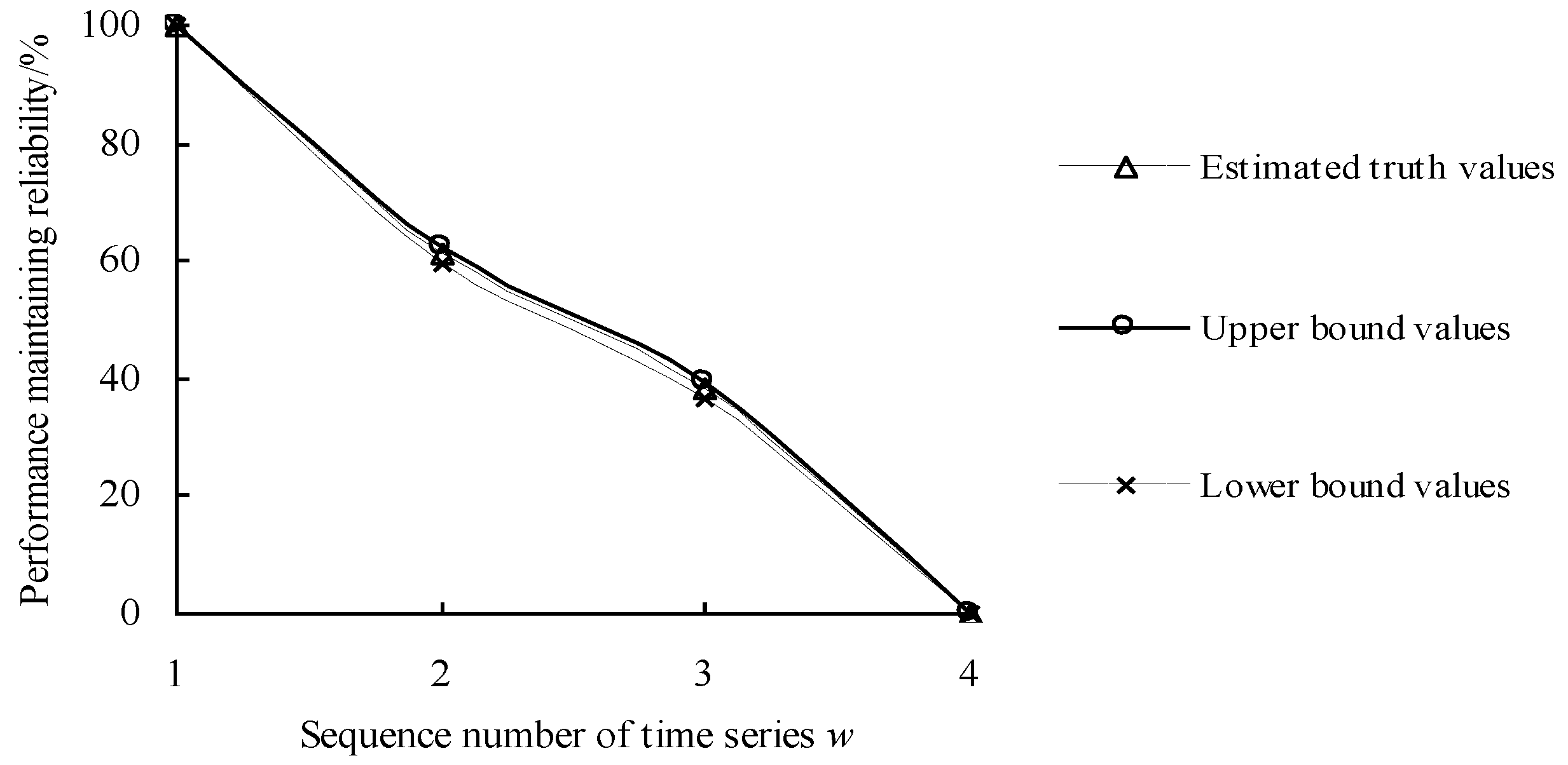
| Sequence Number w | Estimated True Value Rw0/% | Estimated Intervals [R2L, R2U]/% |
|---|---|---|
| 1 | 100 | / |
| 2 | 61.18 | [59.68, 62.39] |
| 3 | 38.13 | [36.71, 39.55] |
| 4 | 0 | / |
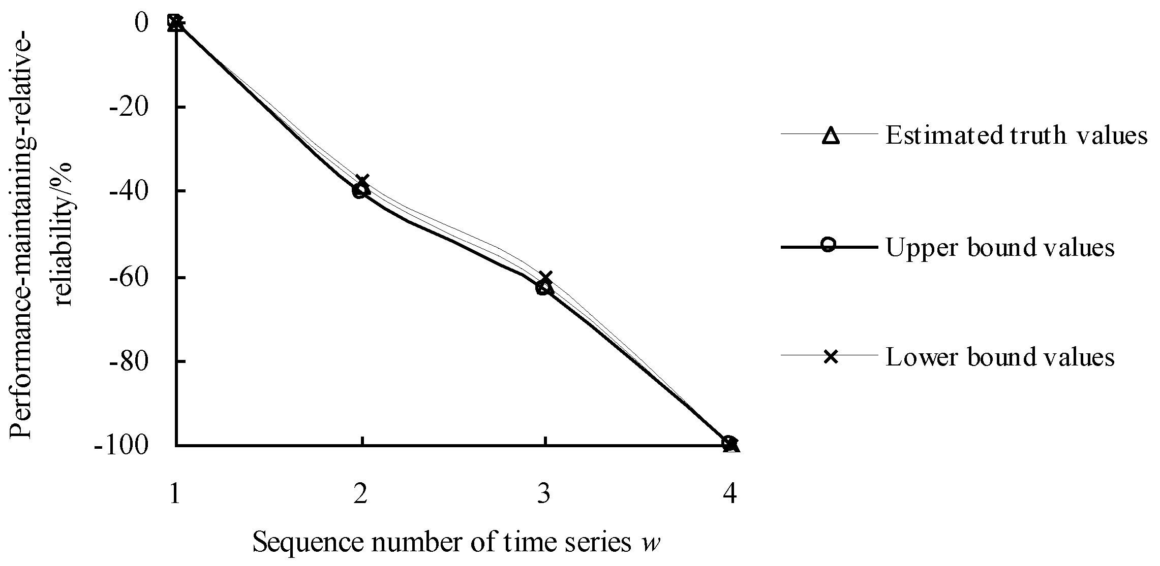
| Sequence Number w | Estimated True Value dw0/% | Estimated Intervals [d2L, d2U]/% |
|---|---|---|
| 1 | 0 | [/, /] |
| 2 | −38.82 | [−40.32, −37.61] |
| 3 | −61.87 | [−63.29, −60.45] |
| 4 | −100 | [/, /] |
| Sequence Number w | Intersection Interval [xw1, xw2]/(m·s−2) | Intersection Area ηw |
|---|---|---|
| 1 | [1.5000, 2.6000] | 1 |
| 2 | [2.2776, /] | 0.6272 |
| 3 | [2.3655, /] | 0.4404 |
| 4 | [/, /] | 0 |
| Sequence Number w | Similarity degrees | |||
|---|---|---|---|---|
| Membership Degree μw | Euclidean Approach Degree β1w | Hamming Approach Degree β2w | Cardinal Approach Degree β3w | |
| 1 | 1 | 1 | 1 | 1 |
| 2 | 0.9053 | 0.8718 | 0.9053 | 0.9503 |
| 3 | 0.7138 | 0.6722 | 0.7138 | 0.8329 |
| 4 | 0.0066 | 0.0049 | 0.0066 | 0.0131 |
| Sequence Number w | Intersection Interval [xw1, xw2]/(m·s−2) | Intersection Area ηw |
|---|---|---|
| 1 | [1.5000, 2.6000] | 1 |
| 2 | [1.7124, 1.9161, 2.2126] | 0.7473 |
| 3 | [1.7431, 1.9981, 2.2740] | 0.6751 |
| 4 | [/, /] | 0 |
| Sequence Number w | Values of PMR/% | ||||
|---|---|---|---|---|---|
| Overlapping Area Method Rw(1) | Membership Degree Method Rw(2) | Hamming Approach Degree Method Rw(3) | Euclidean Approach Degree Method Rw(4) | Cardinal Approach Degree Method Rw(5) | |
| 1 | 100.00 | 100.00 | 100.00 | 100.00 | 100.00 |
| 2 | 64.30 | 72.08 | 71.14 | 72.08 | 73.34 |
| 3 | 57.54 | 62.41 | 61.67 | 62.41 | 64.53 |
| 4 | 0.00 | 0.00 | 0.00 | 0.00 | 0.00 |
| Sequence Number w | Values of PMRR/% | ||||
|---|---|---|---|---|---|
| Overlapping Area Method dw(1) | Membership Degree Method dw(2) | Hamming Approach Degree Method dw(3) | Euclidean Approach Degree Method dw(4) | Cardinal Approach Degree Method dw(5) | |
| 1 | 0 | 0 | 0 | 0 | 0 |
| 2 | −35.7 | −27.92 | −28.86 | −27.92 | −26.66 |
| 3 | −42.46 | −37.59 | −38.33 | −37.59 | −35.47 |
| 4 | −100 | −100 | −100 | −100 | −100 |
| Sequence Number w | Estimated True Value Rw0/% | Estimated Intervals [R2L, R2U]/% |
|---|---|---|
| 1 | 100 | / |
| 2 | 72.16 | [71.02, 73.46] |
| 3 | 62.72 | [61.51, 64.69] |
| 4 | 0 | / |
| Sequence Number w | Estimated True Value dw0/% | Estimated Intervals [d2L, d2U]/% |
|---|---|---|
| 1 | 0 | [/, /] |
| 2 | −27.84 | [−28.98, −26.54] |
| 3 | −37.28 | [−38.49, −35.31] |
| 4 | −100 | [/, /] |
Publisher’s Note: MDPI stays neutral with regard to jurisdictional claims in published maps and institutional affiliations. |
© 2022 by the authors. Licensee MDPI, Basel, Switzerland. This article is an open access article distributed under the terms and conditions of the Creative Commons Attribution (CC BY) license (https://creativecommons.org/licenses/by/4.0/).
Share and Cite
Ye, L.; Hu, Y.; Deng, S.; Zhang, W.; Cui, Y.; Xu, J. A Novel Model for Evaluating the Operation Performance Status of Rolling Bearings Based on Hierarchical Maximum Entropy Bayesian Method. Lubricants 2022, 10, 97. https://0-doi-org.brum.beds.ac.uk/10.3390/lubricants10050097
Ye L, Hu Y, Deng S, Zhang W, Cui Y, Xu J. A Novel Model for Evaluating the Operation Performance Status of Rolling Bearings Based on Hierarchical Maximum Entropy Bayesian Method. Lubricants. 2022; 10(5):97. https://0-doi-org.brum.beds.ac.uk/10.3390/lubricants10050097
Chicago/Turabian StyleYe, Liang, Yusheng Hu, Sier Deng, Wenhu Zhang, Yongcun Cui, and Jia Xu. 2022. "A Novel Model for Evaluating the Operation Performance Status of Rolling Bearings Based on Hierarchical Maximum Entropy Bayesian Method" Lubricants 10, no. 5: 97. https://0-doi-org.brum.beds.ac.uk/10.3390/lubricants10050097