Article

Semi-Supervised Classification of the State of Operation in Self-Lubricating Journal Bearings Using a Random Forest Classifier

AC2T research GmbH, Viktor-Kaplan-Straße 2/C, 2700 Wiener Neustadt, Austria
*
Author to whom correspondence should be addressed.
Submission received: 26 March 2021 / Revised: 30 April 2021 / Accepted: 30 April 2021 / Published: 4 May 2021
(This article belongs to the Special Issue Machine Learning in Tribology)

Abstract

:
For a tribological experiment involving a steel shaft sliding in a self-lubricating bronze bearing, a semi-supervised machine learning method for the classification of the state of operation is proposed. During the translatory oscillating motion, the system may undergo different states of operation from normal to critical, showing self-recovering behaviour. A Random Forest classifier was trained on individual cycles from the lateral force data from four distinct experimental runs in order to distinguish between four states of operation. The labelling of the individual cycles proved to be crucial for a high prediction accuracy of the trained RF classifier. The proposed semi-supervised approach allows choosing within a range between automatically generated labels and full manual labelling by an expert user. The algorithm was at the current state used for ex post classification of the state of operation. Considering the results from the ex post analysis and providing a sufficiently sized training dataset, online classification of the state of operation of a system will be possible. This will allow taking active countermeasures to stabilise the system or to terminate the experiment before major damage occurs.

1. Introduction

Predictive maintenance has been a topic of increasing interest in research and industry over the past few years [1]. As part of predictive maintenance techniques, condition monitoring [2,3,4] is used to detect anomalies and to predict the health of machinery in real time. It uses both sensor data and monitoring software to establish whether a component failure is likely. While some types of failure occur gradually and can be prevented by routine examinations, sudden failures are of course very difficult to forecast. This is the reason why artificial intelligence (AI), especially machine learning (ML) techniques, has gained increasing popularity in the recent years. ML algorithms are trained to learn from the available data and help identify certain behaviours or parameters that contribute to failure with high accuracy. ML algorithms can be divided into two main groups, namely supervised and unsupervised learning [5], differing in whether prior knowledge on the expected output is considered or not. The prerequisite for supervised learning is a set of labelled training data, while unsupervised learning aims at uncovering features on its own.
In tribology research, AI has already been applied to various fields, including in-process tool condition monitoring [3], anomaly detection [6,7,8], failure prediction [9], classification of the lubrication regime [10], optimisation of tribological performance of copper composites [11], as well as AI-based lubricant design [12]. Deshpande et al. [13] give a good summary of the most common machine learning algorithms used in the classification of tribological states of operation and prediction of wear, depending on the application. Classical ML techniques, such as Support Vector Machine (SVM) [3,6,14], Random Forest (RF) [9,15] and Radial Base Function (RBF) methods [16] are widely used. An approach for fast bearing fault diagnosis in rolling elements, combining traditional pattern recognition methods with meta-heuristic search and ML, was presented by Sun et al. [17]. Additionally, deep-learning techniques based on Artificial Neural Networks (ANN) have gained increased popularity over the past few years [10,18,19]. The recently published article by Rosenkranz et al. [20] gives a comprehensive overview of the various application fields and methods in tribology and shows the extended use of AI and ML techniques in the field of tribology as a future perspective.
Acoustic emission (AE), both airborne [8] and structure-borne [9,14], have proven to provide well-suited datasets for training ML algorithms. Other datasets used in tribology-related applications include torque [10] and force [2] data, accelerometer signals [21], as well as images of worn tool surfaces [22]. Thermal imaging has also been applied successfully to fault diagnosis [23].
RF classifiers may have a slightly lower prediction accuracy compared to ANN-based classifiers. However, ANN algorithms require careful parameter tuning and large training datasets. RF classifiers already give good prediction accuracy without or with little fine tuning of their hyperparameters. This makes RF models very suitable for industrial use, as they are easier to adopt for specific applications [24].
In general, self-lubricating sliding elements are composed of porous sintered materials filled with a lubricant [25]. Often, the bearing itself is made out of a porous material, such as sintered metal compounds [26,27,28] or oil-bearing self-lubricating layers [29], as well as polymer composites [30]. Another variant of self-lubricating elements is the use of solid lubricants as coatings, e.g., PTFE in roller bearings [31].
In contrast, the bearings used in this study consist of a base material equipped with a grid of bores, which are filled with a porous polymer compound infiltrated with lubricant. This kind of bearing is common in industrial applications. However, scientific literature on these specific systems is not very widely available; e.g., [32,33], information on this topic is often restricted to company-owned empirical know-how. Consequently, precise knowledge of the main acting mechanisms has not been reported publicly. It is assumed that the variety of commercially available products is based on proprietary know-how and engineering experience.
In 2007, Jisa [34] performed a fundamental review and studied sliding elements in the shape of plates and bearings with different copper-based alloys forming the supporting structure. Jisa has shown that the thermal expansion of the liquid lubricant in the gap between the two sliding components, assisted by capillary effects of the pore and surface topography structures, determine friction levels and lifetime. Generally, the lubricating effect is assisted by a moderate rise of temperature, as the bearing is most likely to operate in boundary or mixed friction conditions. This made a stepwise increase of loading necessary during the run-in phase of the experiment, as a too-high temperature would lead to inferior lubrication due to lower oil viscosity, resulting in adhesive wear and finally end of lifetime by increase of the friction force up to the limit of the specific machine.
For axial sliding operation conditions as studied in the current work, wear is predominantly taking place at the bearing edges and at the edges of the lubricant macrodepots. The wear debris generated at these positions causes abrasive wear in the whole contact zone, leading to gradually growing grooves. As long as the lubricant macrodepots are in contact with the counterbody, these grooves are no lifetime-limiting feature, and most of the wear debris particles are quickly transported out of the contact zone. The re-disposition of wear debris particles into the lubricant macrodepots may lead to a temporary strong increase of the friction force. These events occur rather statistically, accompanied by friction peaks, but they do not result in permanent damage of the lubricant macrodepots and eventually the removal of the loosened wear debris from the sliding contact. Due to these mechanisms, this type of bearings shows self-recovery effects [34].
The judgment of critical operation and useful remaining lifetime in industrial applications relies on specific experience and empirical data exhibiting large variance. The system studied in this work is interesting for application of ML techniques to explore the opportunities of ML for a self-recovering complex tribological system.

2. Materials and Methods

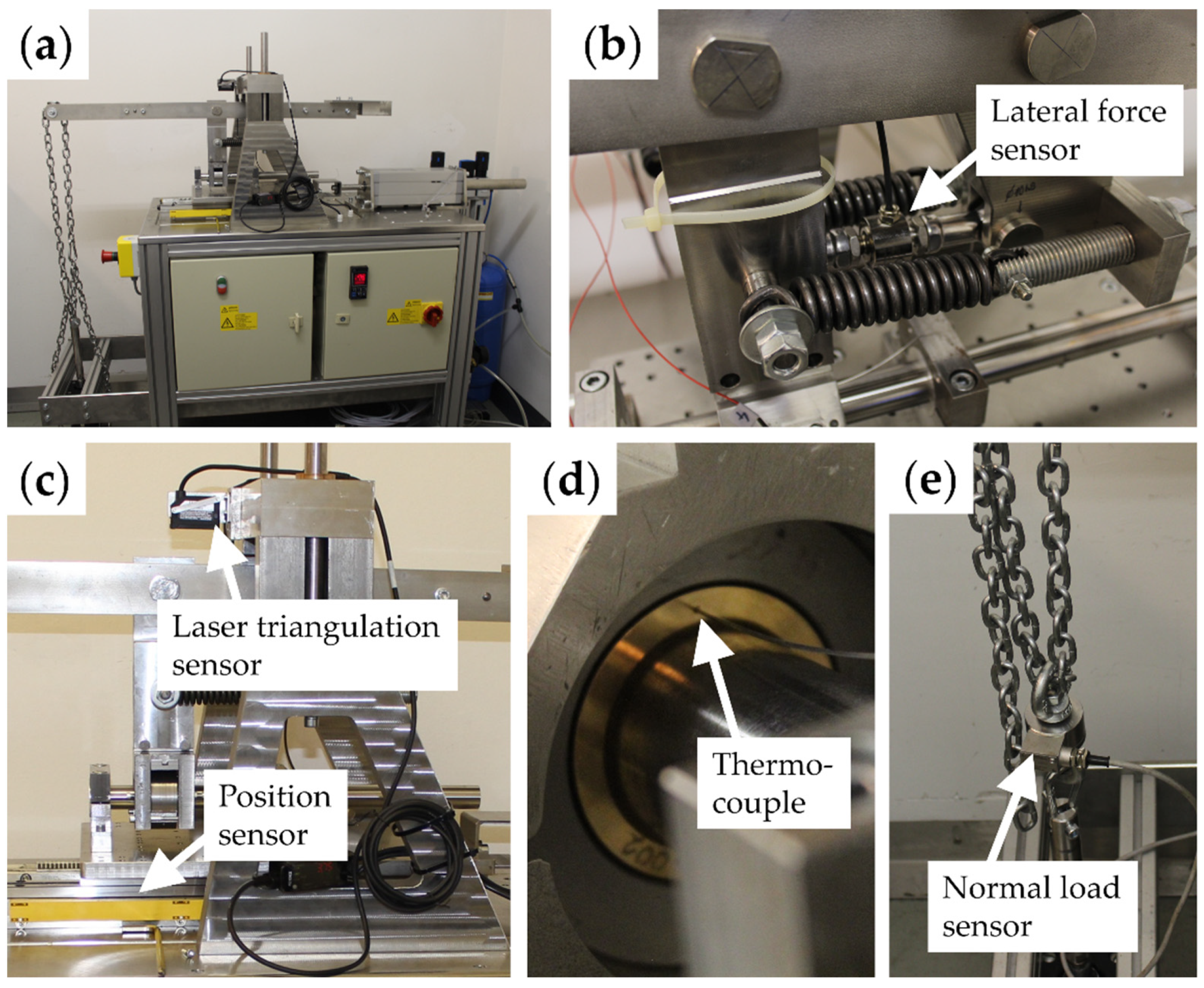
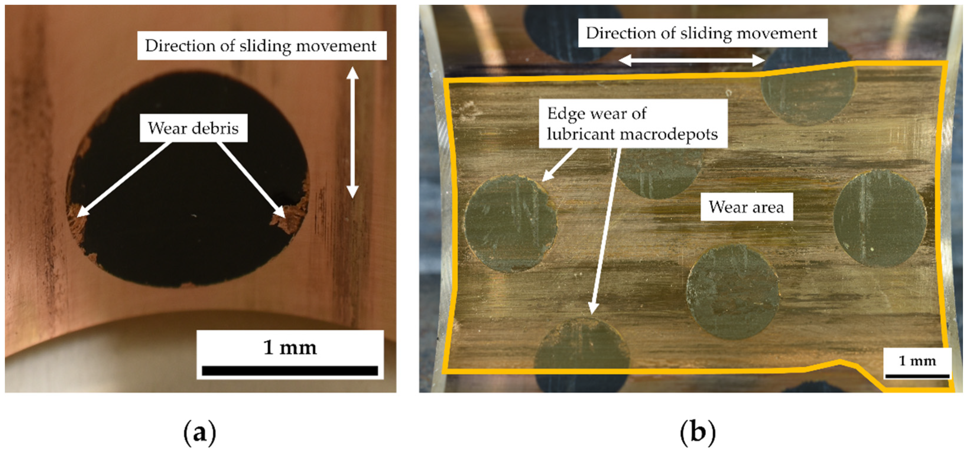
2.1. Experimental Setup

The experiments were performed on a laboratory-built tribometer setup for bidirectional, translatory movements with high normal loads, and large sliding amplitudes (Figure 1a). In this setup, a self-lubricating journal bearing made of a bronze alloy with polymer lubricant macrodepots is horizontally mounted on the tribometer and held in a fixed position. The counterpart, a shaft made of hardened and polished Cr-steel, slides inside this bearing in a translatory oscillating movement driven by a pneumatic cylinder. Two adjustable electronic switches define the reversal points of the oscillating movement. The normal load is applied by a second pneumatic cylinder. The executed force is transmitted via a parallelogram structure, which ensures that the horizontal position of the bearing is always maintained even in the event of wear-induced lowering (Figure 1b). The pressure applied on the bearing was calculated as the normal force acting on the nominal cross-section, according to engineering standards for journal bearings.
The tribometer is equipped with several sensors to monitor and document the defined experimental parameters, the environmental situation, and the reactions of the tribometer to the different friction conditions. The instrumentation of the setup is described in detail below. In the current study, the focus lies on the data generated by the lateral force sensor.
A commercially available linear inductive position sensor (Turck Li300P0-Q17LM0-LiU5X2) measures the oscillating movement of the shaft. The applied normal load and the lateral force, i.e., the force in sliding direction, are recorded by two load sensors (HBM Type U2B and HBM U9C, respectively). The wear of the journal bearing can be qualitatively monitored by the vertical movement of the cantilever, which is measured by a laser triangulation sensor (Keyence IL-030). The temperature of the bearing is measured by a thermocouple (type K, diameter 0.5 mm), which is mounted inside a drilled hole at the top point of the bearing’s front face, where the highest contact pressure and therefore the highest temperature is to be expected. Figure 1 indicates the mounting positions of the force, position, and laser triangulation sensors as well as the thermocouple.
In addition, several sensing techniques are used to detect friction-induced vibrations. Two acoustic emission sensors (NF-Corporation AE-900M-WB), one mounted at the shaft and one mounted at the bearing holder, measure high-frequency structure-borne noise in the range between 100 kHz and 5 MHz. Three MEMS (micro-electro-mechanical system)-acceleration sensors (Analog Devices ADXL1002) are mounted at the bearing holder and detect low-frequency vibrations up to 11 kHz in all spatial directions. The emitted airborne noise is measured in the frequency range between 20 Hz and 20 kHz using a high-precision microphone (Brüel & Kjaer 4189-A-021).
Furthermore, the ambient air temperature and humidity is monitored in the vicinity of the experiment by a TE Connectivity HTM 2500 LF sensing module and the supply air pressure of the pneumatic drive by a Telemecanique XMLP016BC71V pressure transducer.
The oscillation frequency of the shaft was set to a nominal value of 1 Hz and a stroke amplitude of 30 mm, which ensured that each contact point of the shaft was moved out of the contact completely in each stroke. It has to be noted that the oscillation frequency was not constant during the experiment but varied with the resistance the pneumatic cylinder had to overcome to move the shaft. During the first 1.5 h of the experiment, the normal load was gradually increased until a nominal bearing pressure of 8 N/mm2, corresponding to a normal load of 6 kN, was reached. The experiments were performed until at least one of two thresholds was exceeded. The first threshold was set for the bearing temperature at 150 °C and the second one was set for the uncorrected lateral force at ±3.5 kN. However, it should be noted that the temperature threshold was never exceeded, and all experiments were stopped after exceeding the lateral force threshold.
In total, data from 9 experiments performed under the described conditions were used for this study.

2.2. Data Preprocessing

As mentioned above, the sensor measuring the lateral force F L is part of the lever system. In order to obtain the coefficient of friction ( μ ), the geometry of the lever system has to be taken into account, resulting in the following relation:
μ = 100   F L 2   F N 175   F N .
Before feeding the algorithm, several data preprocessing steps were necessary. This was done using the programming language Python in the form of interactive Jupyter notebooks [35], using NumPy arrays [36] and pandas DataFrame objects [37] for efficient computing.
The time-series signals acquired by the force, acceleration, and supplementary sensors, sampled at rates of up to 5 kHz, were stored in the hdf5 file format [38] on a file server dedicated to the storage of large amounts of raw measurement data. Since the amount of raw data was too large for efficient processing on a conventional workstation, data were directly read from the server and downsampled to 100 Hz, thereby carefully retaining the main characteristics of the sensor data.
In a second step, noise was removed from the lateral force and position signals by smoothing with a third-degree Savitzky–Golay filter [39] with a window length of 25 samples.
Due to the oscillating nature of the setup, periodic patterns repeating with the oscillation frequency of the system are present in the lateral force data. Each one of these patterns describes the evolution of the lateral force during one cycle. Deviations from the normal state of operation can be seen as distortions of the individual cycle shapes, which are discussed in more detail in Section 3.1. This leads to an increase in the cycle periods as well as the lateral force levels and maxima.
The zero position of single-cycle curves were triggered using the zero-crossings of the normalised position signal in negative stroke direction. Thus, the length of the extracted curves was normalised to 100 data points per curve using linear interpolation. In the end, an m × 100 matrix, with m being the number of individual cycles of the respective experiment, was obtained as input for the Random Forest classifier.

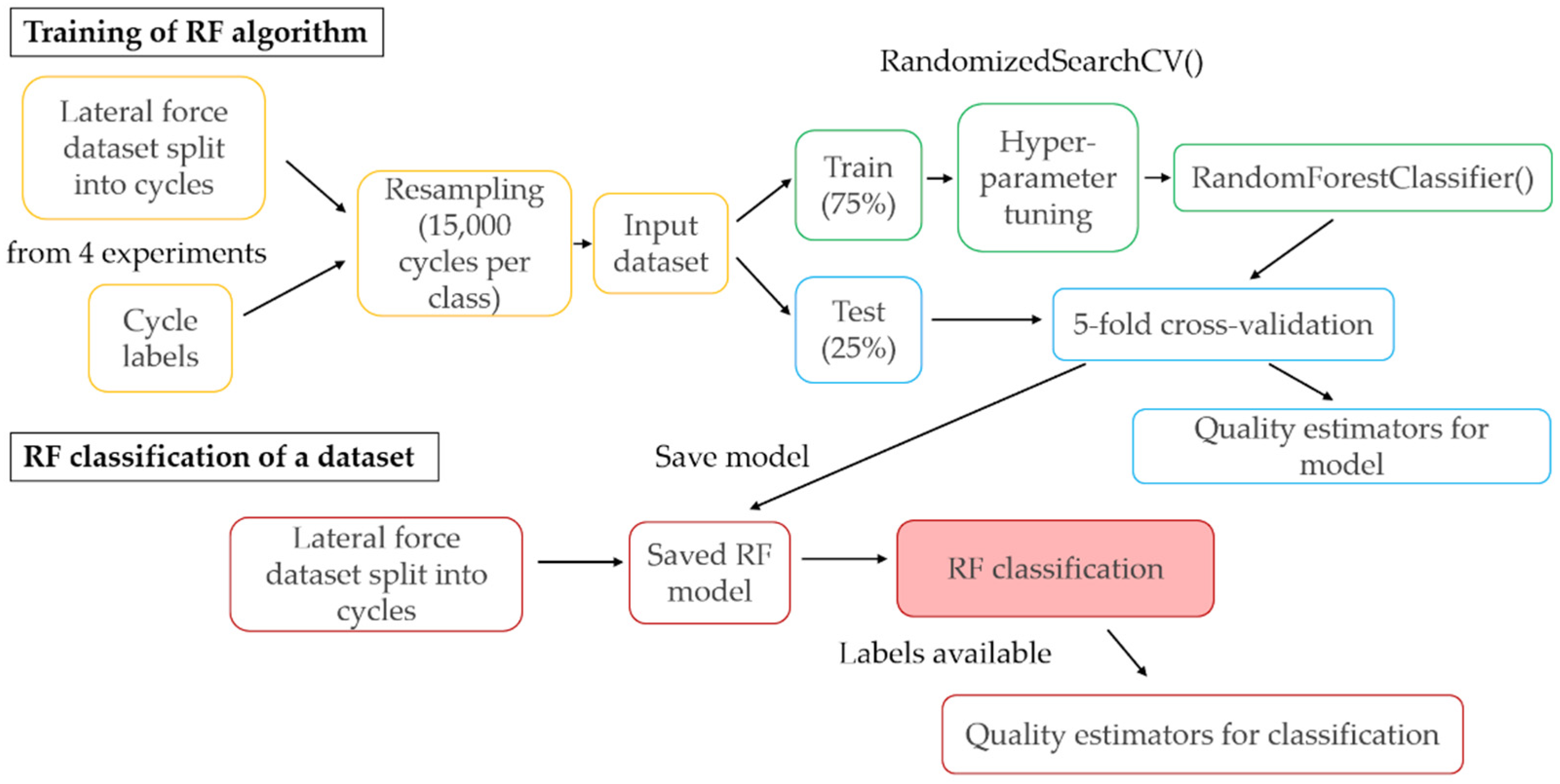
2.3. Random Forest Classifiers

The RF algorithm was first described in detail by Breiman [40]. RF is an ensemble learning algorithm and is based on the aggregation of a large number of independent decision trees. When used for classification, the class votes of each tree determine the classification by majority vote [5], resulting in enhanced classification accuracy and reduced overfitting. Each tree within this RF is grown using random feature selection; each new training set being drawn with replacement from the original training set. This method is known as bootstrap aggregation or bagging [40,41].
In RFs, bagging is combined with a randomised selection of the p input features to be considered for splitting an internal node. At each node, a random subset of k features is selected, from which only the best split is determined [42]. For classification, the default value for k is typically set as the square root of p. At each split, the total reduction in the split criterion, usually measured by the Gini index [43], can be used as an importance measure for the corresponding splitting feature. The feature importance is obtained by accumulating this importance measure over all trees separately for each feature [5]. The size of an individual tree is typically controlled by predefined parameters, such as the terminal node size and tree depth. As a consequence, for every tree in the RF ensemble, a set of observations exists that are not used for growing the tree. These so-called out-of-bag observations (OOB) can be used to estimate the prediction accuracy of the individual decision trees [43].
Generally speaking, the larger the number of estimators, the better the prediction accuracy becomes. However, beyond a critical number of trees, there is no significant performance gain in adding more trees, at the cost of increasing computing demand. Numbers available in the literature include 128 [44], 200 [5], or 250 [45] trees.
In order to assess the prediction quality of the trained RF algorithm, a series of classification metrics is used [46,47].
The most straightforward metric is the accuracy ( q a ), which is defined as the ratio between the number of correct predictions ( N T ) and the total number of samples ( N ), i.e.,
q a = N T N .
If a sample that has been labelled as positive is also predicted as positive, the classification is counted as a True Positive ( N T P ). If it is predicted as negative, the classification is a False Negative ( N F N ). True Negatives ( N T N ) and False Positives ( N F P ) are defined analogously. These four numbers can be displayed as a 2 × 2 confusion matrix C . In the present study, we follow scikit-learn’s implementation [48]; other sources may use the transposed version, e.g., [46].
C = ( N T P N F N N F P N T N ) .
Using above four definitions, the number of correct predictions is given by
N T = N T P + N T N .
The precision ( q p ) or confidence is defined as the fraction of all positively predicted samples ( N P P ), which are actually labelled as positive ( N T P ), i.e.,
q p = N T P N P P = N T P N T P + N F P   .
Conversely, the recall ( q r ) or sensitivity gives the fraction of all positively labelled samples ( N P L ), which are correctly identified as positive, i.e.,
q r = N T P N P L = N T P N T P + N F N   .
In the case of multi-label classification, precision and recall values are calculated separately for each class, with ‘positives’ meaning samples belonging to the respective class. Each row in the confusion matrix represents a ‘true’ class, with the ‘predicted’ class labels as columns. In this case, the confusion matrix contains the number of correct predictions of each class in the diagonal, and false predictions are contained in the respective off-diagonal elements. Given a classification with N labels, the precision and recall can be calculated separately for each class (denoted by index i , i   =   1   N ) from the coefficients of the N × N confusion matrix as follows:
q p ( i ) = C i i j = 1 N C j i
and
q r ( i ) = C i i j = 1 N C i j .

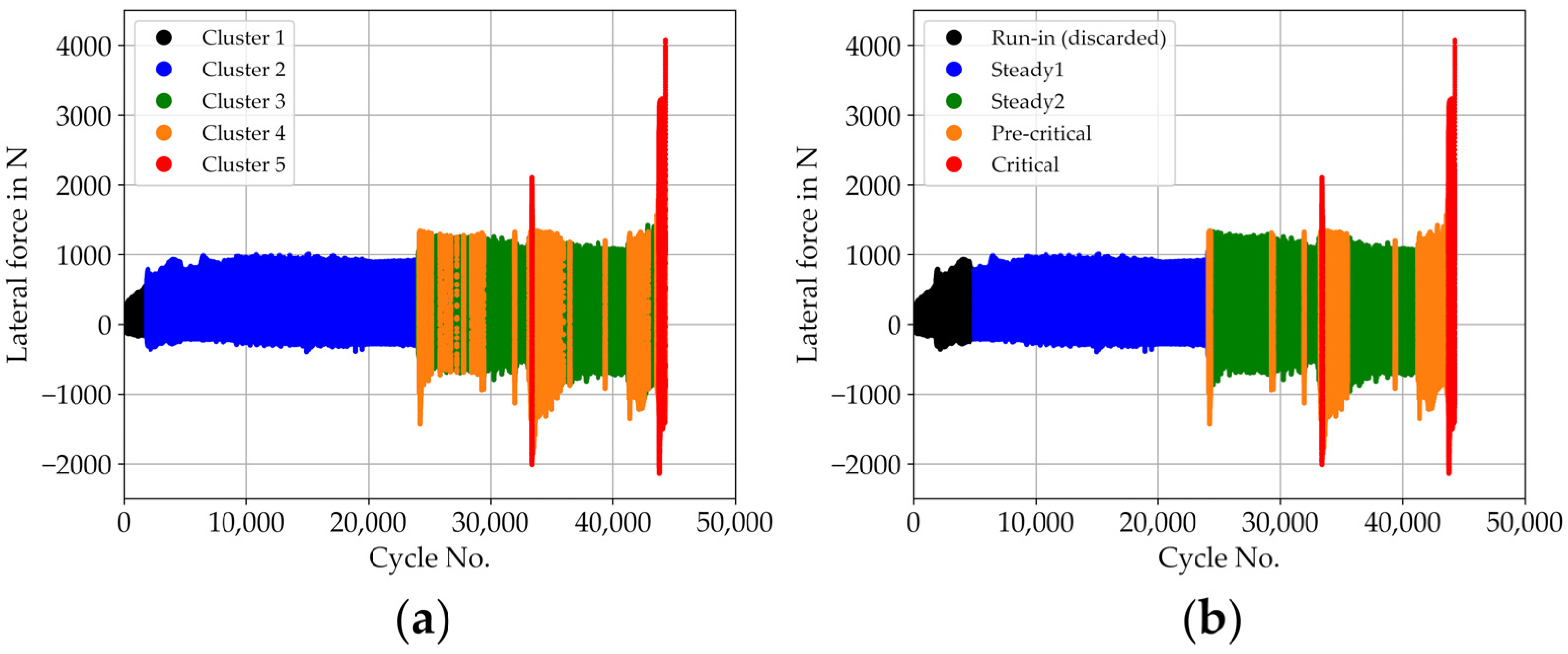
2.4. Labelling of Datasets and RF Model

In this and the following sections, the term ‘state’ refers to the current state of operation on the basis of individual cycles. The term ‘phase’ denotes a longer period of time, in which the system is in a certain state of operation. The term ‘class’ describes a specific categorical label in a set of labels that is assigned to the individual cycles of the dataset during the training period of the RF algorithm, based on their state. Thus, each class consists of a set of individual cycles belonging to one state of operation.
As manual labelling of tens of thousands of cycles would be a very tedious and time-consuming task, a pre-labelling of the cycles via clustering methods was performed. Given the large size of the data, Principal Components Analysis (PCA) was applied to reduce the dimensionality of the input and visualise the general shape of the data. After selecting an appropriate number of principal components, based on the amount of variance covered, a k-means clustering algorithm was applied to the reduced dataset. Each cycle was assigned to a cluster such that the squared Euclidean distances within each cluster were minimised. The implementations of these two steps were performed in R using the prcomp and kmeans functions [49].
The results of this pre-labelling stage are given in Table 1. Before applying PCA, the datasets were centred and scaled to have unit variance. For the k-means clustering, the first two principal components were selected, showing cumulative proportions of variance between 0.79 and 0.93. The number of clusters for the k-means algorithm was set to 5, based on the expected tribological regimes of the studied tribological experiment. The resulting cluster sizes for each experiment are unevenly distributed, as can be seen in Table 1.
The clusters were subsequently assigned to tribological states of operation: ‘Steady1’, ‘Steady2’, ‘Pre-critical’, and ‘Critical’. The first 5000 cycles were defined ‘Run-in’ and discarded due to the high variability of the data. The preliminary labelling was refined in a second step by closer inspection of the data, taking into account distinctive features in the other sensor signals, e.g., sudden temperature increases or distortions of the position signal. This resulted in the inclusion of additional ‘Pre-critical’ areas–typically before and after short-term (‘Critical’) anomalies or before critical operation at the end of the experiments as well as physically meaningful merging of regions fragmented into various states of operation by the clustering algorithm. Figure 2 shows the comparison of the classification obtained by k-means clustering and the final labelling for one of the experiments used for training the RF algorithm. Here, single cycles or groups of cycles that did not differ significantly from their surroundings, which were marked as ‘Pre-critical’ (cluster 4) by the k-means clustering, were assigned to the respective steady state. Furthermore, the area preceding the final critical state was labelled as ‘Pre-critical’ in its entirety, while the k-means result switched between ‘Pre-critical’ and ‘Steady2’ in this region. This led to an overall increase of cycles labelled as ‘Pre-critical’ after manual adaptation (see Table 2). The ‘Steady1’ state is reduced in size after manual adaptation, as the first 5000 cycles were discarded.
In the end, four classes representing the individual states of operation were distinguished; see Figure 3. ‘Steady1’ was used for steady operation, typically right after the run-in period, with little fluctuation and few distortions in the data. ‘Steady2’ typically occurred after major events. The system stabilises, but higher lateral forces are measured, and the curve shapes of the cycles are more distorted and variable. After sufficient running time without major events, the system may reach the ‘Steady1’ state again. ‘Pre-critical’ cycles are typically found before and after cycles labelled as ‘Critical’. The ‘Pre-critical’ label is also associated with short-time events, typically lasting less than 100 cycles. During these short-time events, maximum lateral force values of 1.5 times the maxima of the surrounding steady-state cycles or lager were measured. ‘Critical’ cycles show heavily distorted curves with the lateral force increasing considerably at one or both turning points. This indicates that the bearing was stuck in its turning position and could only be brought back into motion when a sufficiently high lateral force was applied. One has to note that the x-axis in the graphs of Figure 3 corresponds to a relative position in time within each cycle rather than the actual physical encoder position. The length of the half-cycle, in which the deadlock occurred (the case for the positive half-cycle is depicted in Figure 3d), is extended, leading to an overall asymmetric cycle shape. As all cycles were normalised to a length of 100 data points, the steepness of the lateral force curve in the turning points is related to the cycle duration, which itself depends on the friction in the system at that moment.
The RF algorithm was developed using the Python ML package scikit-learn [48]. The workflow for training and application of the algorithm is described in detail below, and the corresponding flowchart is shown in Figure 4.
The dataset for training the algorithm was created using labelled cycles from four experiments, namely the numbers 2, 4, 7, and 9 in Table 1. As mentioned above, the first 5000 cycles from each experiment were considered as run-in and discarded from the dataset. Data from multiple experiments were chosen in order to cover the diversity of cycle shapes within each state and to equalise bias towards a certain state introduced by manual labelling. This includes, above all, the distortions introduced by pre-critical and critical operation, which can happen in either positive, negative, or both stroke directions.
As the distribution of the cycles over the classes representing the four states of operation was highly unbalanced (see Table 3), each class was resampled to a size of 15,000 cycles by random selection with replacement. That means that the classes ‘Steady1’, ‘Steady2’, and ‘Pre-critical’ were downsampled, and a random selection of the cycles over all four experiments was used for training. However, the size of the class representing the ‘Critical’ state was only 1265 cycles and had to be upsampled by a factor of nearly 12, drawing each cycle multiple times from the dataset. The number of 15,000 cycles was chosen, as it seemed to be a good compromise between retaining as much information as possible from the three larger classes and keeping the upsampling factor of the ‘Critical’ class reasonably small.
Before training the RF algorithm, a randomised hyperparameter tuning was performed using scikit-learn’s RandomizedSearchCV function in order to optimise the following hyperparameters. Randomised hyperparameter tuning has the advantage of a fixed, pre-defined number of trials, independent of the total number of combinations, which can be very large. This strategy will find a near-best combination of hyperparameters at the advantage of not spending too much time on unpromising candidates [50]. For the present work, the number of iterations was set to 100. The following hyperparameters were optimised using randomised hyperparameter tuning: n_estimators indicates the number of individual decision trees in the RF, min_samples_split is the minimum number of samples to split an internal node, min_samples_leaf is the minimum number of samples required to be in a leaf node, max_features is the maximum number of features to consider at each split and was always set to the square root of the total number of features; i.e., 10, max_depth indicates the maximum number of levels within an individual decision tree and finally, bootstrap = True means that bootstrap samples are used to build each tree rather than the whole dataset. Table 4 shows the best obtained set of hyperparameters, which were subsequently used for training the algorithm.
The RF algorithm was trained using 75% of the input dataset as training data and 25% as test data used for determination of the quality estimators described in Section 2.3. Then, the prediction accuracy of the trained RF algorithm was assessed by a 5-fold cross-validation with random selection of cycles for the training and test dataset. Data were again split into 75% training and 25% test data for each run, which were randomly selected from the input dataset. Finally, the algorithm was validated on a labelled experiment (number 8 in Table 1), which was not used for training.

3. Results

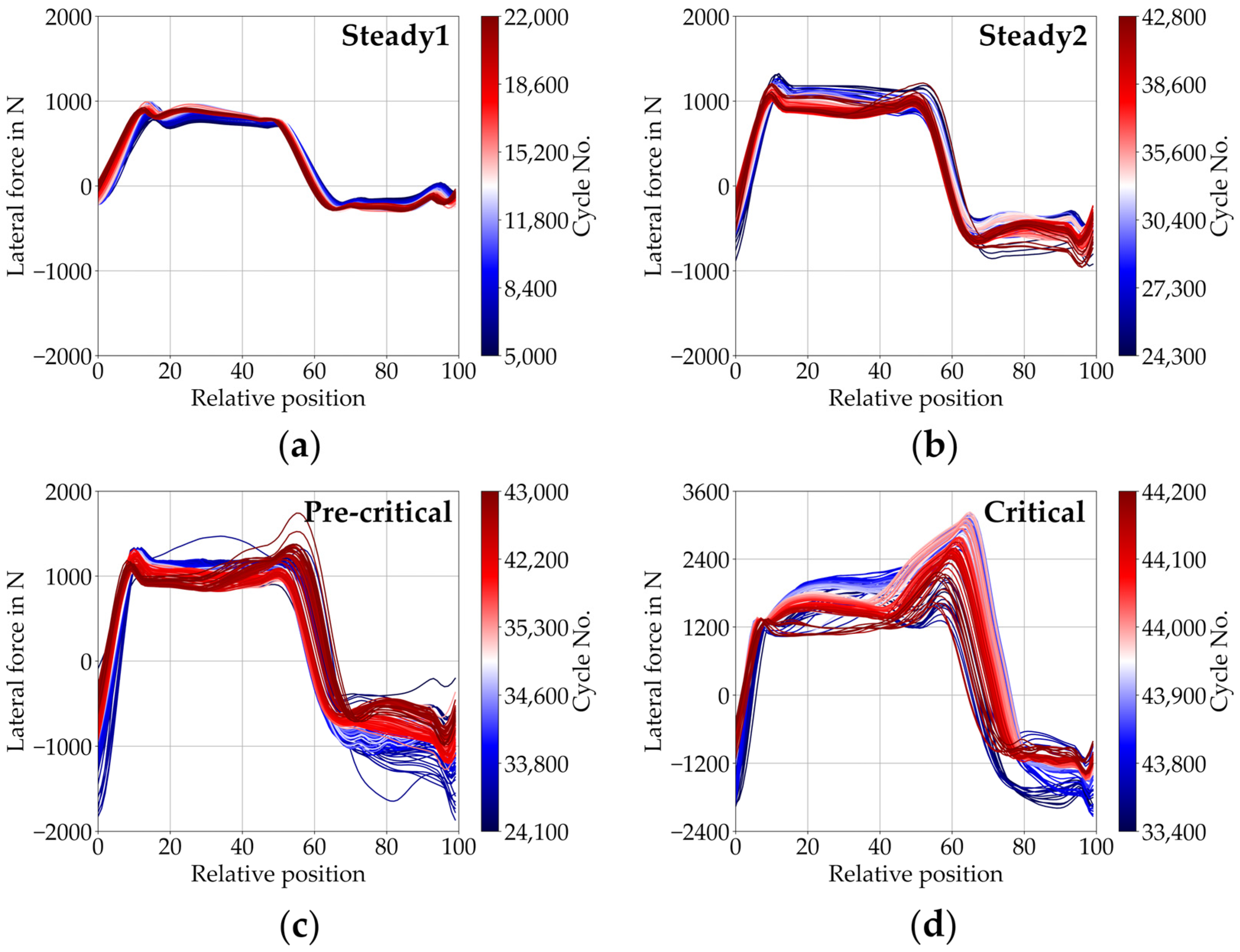
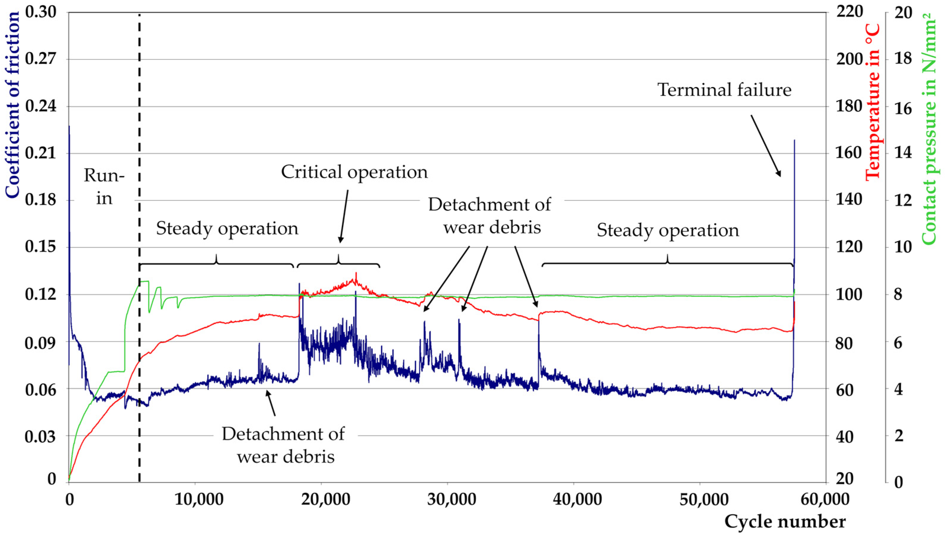
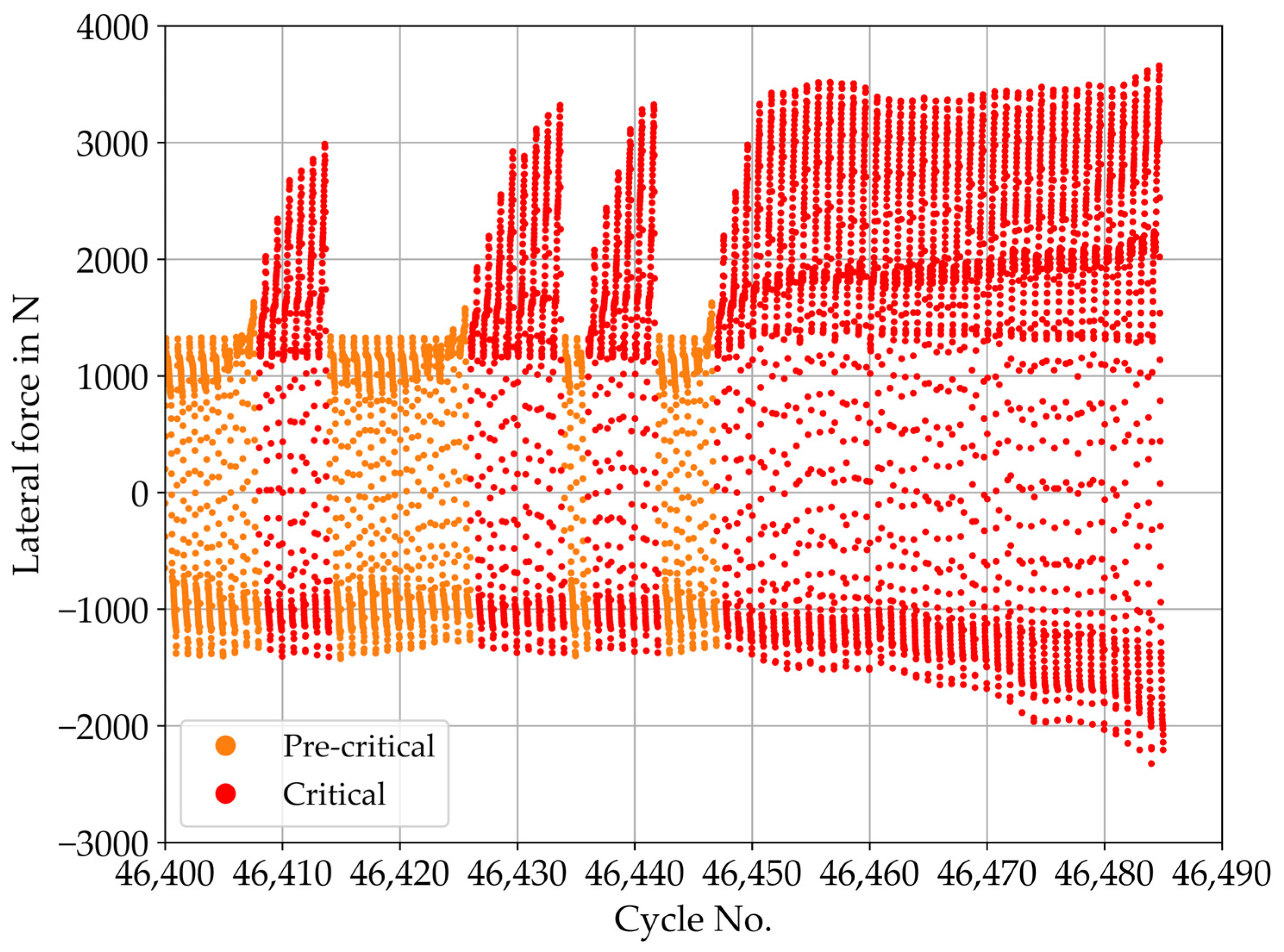
3.1. Frictional Behaviour

The average duration of an experiment until reaching the stop criterion was 14.5 ± 2.6 h, corresponding to roughly 44,170 ± 7400 cycles.
Although the temporal evolution of the measured signals varied between the experiments, a few characteristic features were observed throughout the experiments. Figure 5 shows the time series of coefficient of friction, temperature, and contact pressure of experiment 4 as an example for characteristic features observed during the series of experiments. For the coefficient of friction, the arithmetic means of the absolute values of the 10% and the 90% quantiles are displayed. The 10% quantile gives a characteristic value for the coefficient of friction in negative stroke direction, whereas the 90% quantile was used for the positive direction.
After the run-in, the system was operating in a stable condition at a mean coefficient of friction of around 0.06, with the temperature steadily increasing close to 90 °C. After typically 15,000 to 30,000 cycles, a region of pre-critical and critical operation was observed. This manifests itself in a sudden increase in the coefficient of friction and the temperature exceeding 100 °C. This may be attributed to locally inferior lubrication and consequently short-time metal-to-metal contact and adhesion. After a few minutes, the system was able to loosen the adhesive contact spot or to tear off a machining chip from the edge of a lubricant macrodepot. After that, the system remained in the pre-critical state, self-healed, and thus slowly returning to steady operation, albeit at a slightly higher coefficient of friction in most cases, typically between 0.07 and 0.10. The eventual steady increase of the coefficient of friction can be attributed to the gradually deteriorating lubricant supply due to capillary forces, which reduce due to the increasing number and depth of abrasive grooves caused by wear particles. The short-time critical states with subsequent stabilisation of the system due to self-recovery could be observed repeatedly in all experiments.
During the experiment, spikes in the friction curves were observed. In order to investigate the origin of these spikes, additional experiments were carried out and stopped manually when the first spike occurred. Investigation of the bearing revealed that these spikes were most likely caused by wear debris in the form of tiny machining chips detached from the edge of a lubricant macrodepot and subsequently transported further in the contact zone to be either embedded within another lubricant macrodepot or transported out of the contact at the edges of the sliding element; see Figure 6a. Figure 6b indicates the large extent of the clearly visible wear area on the self-lubricating journal bearing after the experiment.
Prior to reaching the set threshold criteria of the system by reaching a given lateral force, four experiments exhibited an extended instable state, which lasted for up to several thousand cycles. However, in the other five experiments, the stop criterion was reached almost instantaneously, with instable operation of less than 10 min before termination of the experiment. Experiment 4, as shown in Figure 5, belongs to the latter category. In experiment 6, no intermediary critical operation was observed. The system remained steady for about 10 h, with a sudden increase of the lateral force in the end, exceeding the stop criterion. Experiment 3 was manually terminated after about 2 h of pre-critical operation, before reaching the stop criterion.

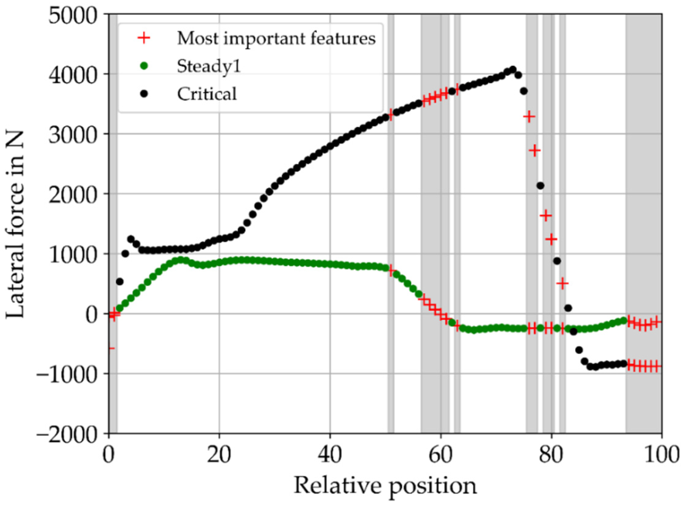
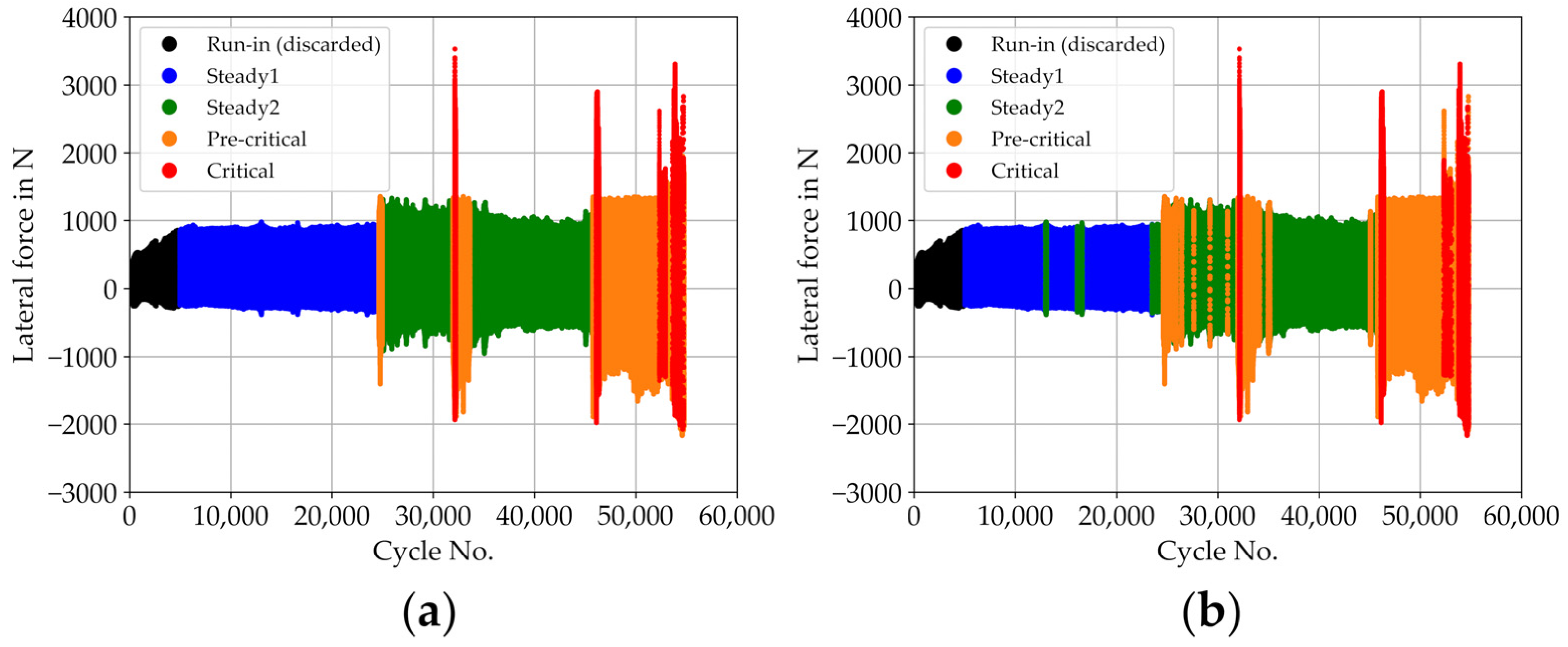
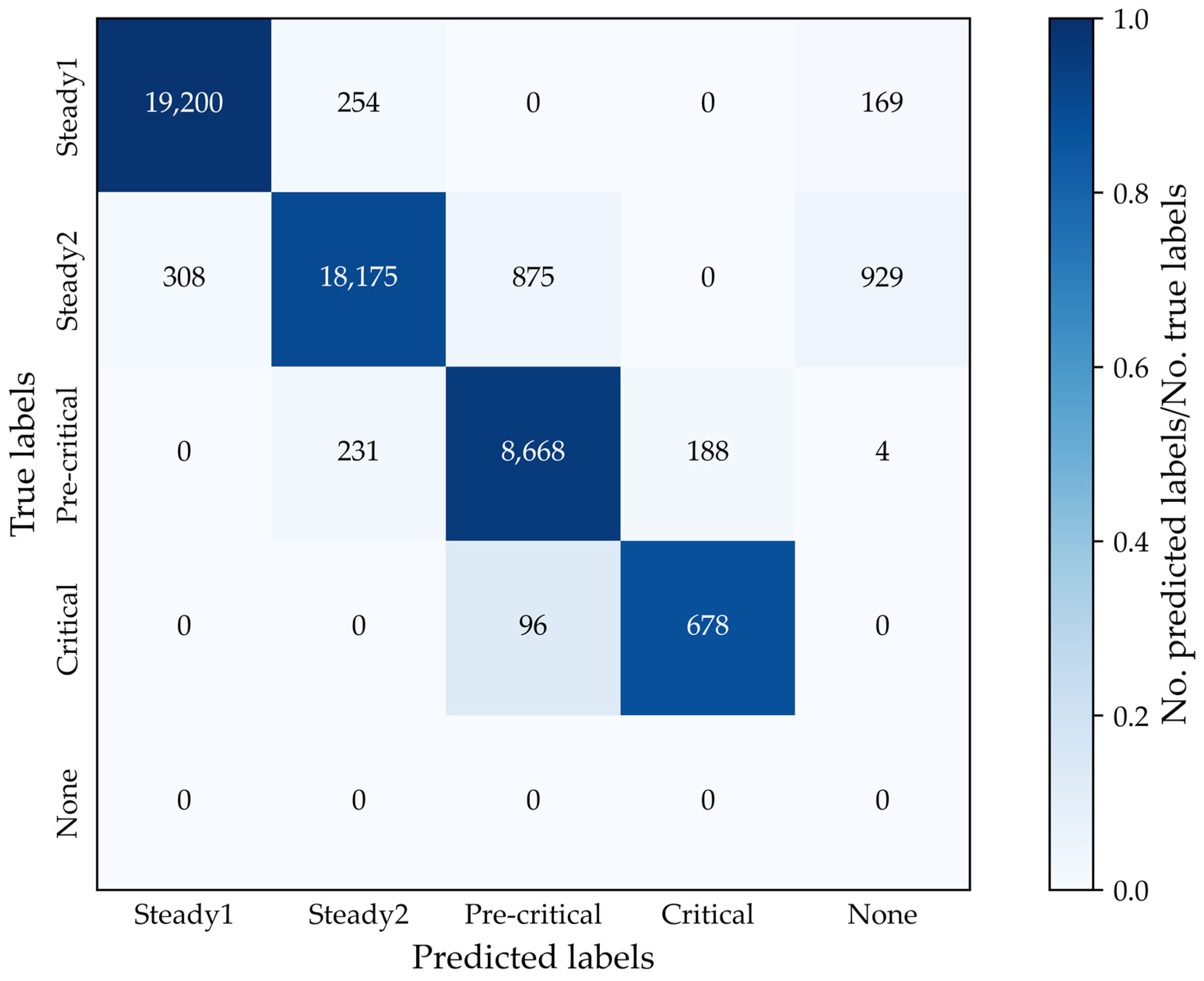
3.2. Classification of States of Operation

The prediction accuracy of the trained RF model was determined to be 0.991, corresponding to an OOB score of 0.996. Five-fold cross-validation yielded a mean prediction accuracy of the model of 0.993 ± 0.001. These values indicate a classification error rate between 0.5% and 1%.
Figure 7 shows the locations of the 20 most important features used for splitting nodes in the RF model. The x-axis label ‘Relative position’ refers to a relative position in time during the duration of one stroke rather than an actual physical position. One can see clearly that the most important areas are located around the two turning points of the stroke direction of the steady-state cycles, i.e., around 60 for the change between positive and negative stroke and around 100 or 0 for the change from negative to positive. Another region, where important features are located, can be found around 80, corresponding to the location of turning points of the critical cycles in the positive stroke direction. The feature around 50 may be associated with critical cycles in the negative stroke direction.
In order to assess the prediction quality of the RF algorithm on other datasets, the dataset of experiment 8, which was not used for training the RF algorithm, was labelled according to the procedure described above, and classification metrics were calculated. A comparison between the labels assigned to each cycle and the labels predicted by the RF algorithm is shown in Figure 8.
The overall classification accuracy of experiment 8 was 0.939. Table 5 shows the precision and recall values for the four classes. Both steady states as well as the pre-critical state were recognised with high precision and recall. Of the cycles classified by the algorithm as ‘Critical’, only 78% were actually labelled as ‘Critical’. The remaining 12%, or 188 cycles, had the true label ‘Pre-critical’. However, 88% of the actual states labelled as ‘Critical’ were identified correctly. The corresponding absolute values are shown in the confusion matrix in Figure 9. The colour scale indicates the fraction between predicted labels and the total number of true labels assigned to the respective class, summing up to 1 for each row. For the diagonal elements, this corresponds to the recall. The last row and column, labelled as ‘None’, indicates cycles, for which the algorithm was not able to issue a prediction. This was predominantly the case for the two steady states, with about 4.5% of the cycles labelled ‘Steady2’ not classified. This is also the reason for the relatively low recall of 0.9 for this class.
Based on the results of the RF classification, Table 6 shows a summary of the lengths of the pre-critical phases preceding the end of the respective experiment. As already mentioned, the experiments could be divided in two distinctly different groups according to their behaviour towards the end of the experiment. In the first group, an extended pre-critical phase was observed before the termination of the experiment. This pre-critical phase was found to last between 60 and 211 min or between 7.4 and 19.2% of the total running time. Before reaching the stop criterion, individual critical cycles were observed during the pre-critical phase, with an increasing abundance of critical cycles towards the end, as shown in Figure 10.
The second group shows a pre-critical and critical operation rather suddenly. The stop criterion was exceeded within less than 10 min. Experiment 6 reached pre-critical operation as few as 1.5 min before termination of the experiment. This sudden critical behaviour may be due to a sudden loss of the lubricant supply, resulting in a pronounced increase in the lateral force, whereas in the first group, lubricant supply was sufficient to keep the system in an operable state over a longer period.

4. Discussion

This paper presents a semi-supervised method for the classification of states of operation during a tribological sliding experiment in oscillating, translatory motion using an RF classifier.
An RF classifier was selected due to its low complexity regarding implementation, its good prediction accuracies, and the low requirements for model tuning. The RF model can be easily trained, validated, and applied on a local machine, with the capability of real-time classification. RF classifiers are especially well suited for industrial applications, as no AI expert is required to set up and tune sophisticated ANN-based algorithms [24].
The algorithm was trained on the basis of individual cycles. This is only possible if the force data are recorded with high temporal resolution. The trained algorithm was able to classify the state of operation with an accuracy of 0.939 for data of a labelled test experiment, using samples from four different experimental runs (i.e., four different journal bearings with otherwise identical experimental setup) as the training dataset.
The proposed methodology can be extended to similar systems, with different dimensions and materials of the involved bodies. However, datasets from these systems are necessary for training the algorithm. The transfer of an already trained algorithm to other systems remains an aspect for further investigation.
As a future perspective, online classification of the current status of the system will help to identify critical operation conditions. This will allow taking real-time countermeasures to assist the self-recovering process of the system, such as reduction of oscillation frequency or normal load, up to stopping the experiment to prevent major damage. The experiment can be stopped during critical operation for ex post analysis, e.g., material or surface analysis of the sliding bodies. Detailed knowledge of the system and its history can be used to define more complex stopping criteria, additionally to simple threshold values.
The presented approach may be extended to applications in industrial machinery, provided that a continuous force measurement and a sufficient amount of training data from ex post analysis are available. Examples for potential industrial applications range from journal bearings mounted in industrial equipment or drive trains to hydraulic presses, pistons, and manufacturing tools, especially where the accessibility of the system is limited for optical inspection.
In a further step, the presented algorithm may form a basis for lifetime prediction. Experimentally determined durations until reaching the stop criteria and thus termination of the experiment may be used as additional input for training the algorithm. This is a challenging task, as terminal failure often occurs suddenly without showing progressive deterioration in advance [9]. In the present work, sudden terminal failure occurred in about half of the analysed experiments. In the other experiments, terminal failure was preceded by pre-critical operation of up to 3.5 h. Inclusion of further continuous sensor data, such as temperature, acceleration, airborne or structure-borne AE, may serve to improve labelling and provide additional information for lifetime prediction. With a combination of these sensors, training of a similar RF algorithm is possible, even if no continuous force data are available.
In contrast to most studies regarding ML in tribological applications, in the current study, a self-recovering system was analysed. Thus, the system may stabilise after a pre-critical or even critical phase and return to steady operation. For conventional tribological systems, pre-critical or critical operation indicates an impending failure of the system, and stopping the experiment is the only way to prevent major damages. For self-recovering systems, an online ML algorithm will have to distinguish between transient and terminal critical operation. To achieve that, additional datasets such as AE or acceleration data have to be included.
A high quality of the labels assigned to the training dataset has proven to be the key for a high prediction accuracy of the RF algorithm. The presented semi-supervised approach—labelling by unsupervised k-means clustering with manual refinement—offers the flexibility to choose within a range between fully automated, unsupervised labelling and entirely manual labelling based on expert knowledge. In order to provide high-quality labelled training datasets, tribological and engineering expertise have to be included in the classification process in any case.
There are several papers on friction and wear monitoring as well as failure classification using data from AE sensors, e.g., [9,14,51] or image data, including optical [22] and thermal imaging [23]. In contrast, the proposed method focuses on time-series data from a force sensor collected at sampling rate of 5 kHz, similar to e.g., [2], as a data source for training a ML algorithm. This has the great advantage that high classification accuracy can be reached by using only force data, recorded by default in any tribological experiment. However, time-series data from other sensors, such as AE or acceleration, and optical or thermal image data, can provide useful additional information, which can be used to increase the algorithm’s classification accuracy.
The focus of the current work was set to the overall health condition of the bearing, which can be characterised by its state of operation, ultimately related to wear and lubrication in the contact area. As a system of self-lubricating journal bearings exhibits the ability for self-recovery during usage, it could be shown that the presented RF classifier allows detecting critical conditions prior to the onset of machine failure, solely based on the lateral force data. Future research will address the prediction of useful remaining lifetime and ultimate system failure.

5. Conclusions

In this paper, an oscillating, translatory sliding experiment of a self-lubricating bronze journal bearing, which provides the system with the ability to self-recover minor damages, was studied to elaborate a semi-supervised ML algorithm predicting critical operating conditions. An RF classifier was trained on the basis of single cycles of lateral force signals acquired with high resolution and including expertise knowledge of tribologists. Four different states of operation were identified based on the shape of the cycles. The main findings of the present paper are as follows:
  • An RF algorithm, trained with high-resolution force signals of four experiments, showed a high degree of classification accuracy (0.939) after validation against a labelled dataset of another experiment.
  • The labelling step is essential and preferably includes tribological expert knowledge. The proposed method offers the flexibility to choose within a range between fully automated and fully expert-related labelling.
  • The application of a pre-trained algorithm to unlabelled data is very efficient and therefore can be used for immediate countermeasures to assist the self-recovering process of the system or to prevent major damage.

Author Contributions

Conceptualisation: U.C.-B. and F.P., data curation: J.P. and G.V., formal analysis: J.P., G.V. and I.A.N., methodology: U.C.-B., R.G., J.P. and G.V., project administration: J.P., software: J.P., supervision: G.V., validation: J.P., visualisation: J.P., writing—original draft preparation: J.P., R.G. and I.A.N., writing—review and editing: U.C.-B., F.P. and G.V. All authors have read and agreed to the published version of the manuscript.

Funding

This work was funded by the Austrian COMET Program (project InTribology1, No. 872176) via the Austrian Research Promotion Agency (FFG) and the Provinces of Niederösterreich and Vorarlberg and has been carried out within the Austrian Excellence Centre of Tribology (AC2T research GmbH).

Institutional Review Board Statement

Not applicable.

Informed Consent Statement

Not applicable.

Data Availability Statement

The data presented in this work are available on request from the corresponding author.

Conflicts of Interest

The authors declare no conflict of interest.

References

  1. Pech, M.; Vrchota, J.; Bednář, J. Predictive Maintenance and Intelligent Sensors in Smart Factory: Review. Sensors 2021, 21, 1470. [Google Scholar] [CrossRef] [PubMed]
  2. Gouarir, A.; Martínez-Arellano, G.; Terrazas, G.; Benardos, P.; Ratchev, S. In-process Tool Wear Prediction System Based on Machine Learning Techniques and Force Analysis. Procedia CIRP 2018, 77, 501–504. [Google Scholar] [CrossRef]
  3. Pandiyan, V.; Caesarendra, W.; Tjahjowidodo, T.; Tan, H.H. In-process tool condition monitoring in compliant abrasive belt grinding process using support vector machine and genetic algorithm. J. Manuf. Process. 2018, 31, 199–213. [Google Scholar] [CrossRef]
  4. Avendano, D.N.; Caljouw, D.; Deschrijver, D.; Van Hoecke, S. Anomaly detection and event mining in cold forming manufacturing processes. Int. J. Adv. Manuf. Technol. 2020, 1–16. [Google Scholar] [CrossRef]
  5. Hastie, T.; Tibshirani, R.; Friedman, J. The Elements of Statistical Learning: Data Mining, Inference, and Prediction, 2nd ed.; Springer: New York, NY, USA, 2009. [Google Scholar]
  6. Saeidi, F.; Shevchik, S.; Wasmer, K. Automatic detection of scuffing using acoustic emission. Tribol. Int. 2016, 94, 112–117. [Google Scholar] [CrossRef]
  7. König, F.; Sous, C.; Chaib, A.O.; Jacobs, G. Machine learning based anomaly detection and classification of acoustic emission events for wear monitoring in sliding bearing systems. Tribol. Int. 2021, 155, 106811. [Google Scholar] [CrossRef]
  8. Pandiyan, V.; Prost, J.; Vorlaufer, G.; Varga, M.; Wasmer, K. Identification of Abnormal Tribological Regimes Using a Mi-crophone And Semi-Supervised Machine-Learning Algorithm. Friction 2021. accepted for publication on 3 April 2021. [Google Scholar]
  9. Shevchik, S.A.; Saeidi, F.; Meylan, B.; Wasmer, K. Prediction of Failure in Lubricated Surfaces Using Acoustic Time–Frequency Features and Random Forest Algorithm. IEEE Trans. Ind. Inform. 2016, 13, 1541–1553. [Google Scholar] [CrossRef]
  10. Moder, J.; Bergmann, P.; Grün, F. Lubrication Regime Classification of Hydrodynamic Journal Bearings by Machine Learning Using Torque Data. Lubricants 2018, 6, 108. [Google Scholar] [CrossRef] [Green Version]
  11. Thankachan, T.; Prakash, K.S.; Kamarthin, M. Optimizing the Tribological Behavior of Hybrid Copper Surface Composites Using Statistical and Machine Learning Techniques. J. Tribol. 2018, 140, 031610. [Google Scholar] [CrossRef]
  12. Bhaumik, S.; Mathew, B.R.; Datta, S. Computational intelligence-based design of lubricant with vegetable oil blend and various nano friction modifiers. Fuel 2019, 241, 733–743. [Google Scholar] [CrossRef]
  13. Deshpande, P.; Pandiyan, V.; Meylan, B.; Wasmer, K. Acoustic emission and machine learning based classification of wear generated using a pin-on-disc tribometer equipped with a digital holographic microscope. Wear 2021, 203622, 203622. [Google Scholar] [CrossRef]
  14. Mokhtari, N.; Pelham, J.G.; Nowoisky, S.; Bote-Garcia, J.-L.; Gühmann, C. Friction and Wear Monitoring Methods for Journal Bearings of Geared Turbofans Based on Acoustic Emission Signals and Machine Learning. Lubricants 2020, 8, 29. [Google Scholar] [CrossRef] [Green Version]
  15. Bustillo, A.; Pimenov, D.Y.; Mia, M.; Kapłonek, W. Machine-learning for automatic prediction of flatness deviation considering the wear of the face mill teeth. J. Intell. Manuf. 2021, 32, 895–912. [Google Scholar] [CrossRef]
  16. Boidi, G.; Da Silva, M.R.; Profito, F.J.; Machado, I.F. Using Machine Learning Radial Basis Function (RBF) Method for Predicting Lubricated Friction on Textured and Porous Surfaces. Surf. Topogr. Metrol. Prop. 2020, 8, 044002. [Google Scholar] [CrossRef]
  17. Sun, S.; Przystupa, K.; Wei, M.; Yu, H.; Ye, Z.; Kochan, O. Fast bearing fault diagnosis of rolling element using Lévy Moth-Flame optimization algorithm and Naive Bayes. Ekspolatacja Niezawodn. Maint. Reliab. 2020, 22, 730–740. [Google Scholar] [CrossRef]
  18. Argatov, I. Artificial Neural Networks (ANNs) as a Novel Modeling Technique in Tribology. Front. Mech. Eng. 2019, 5, 5. [Google Scholar] [CrossRef] [Green Version]
  19. Souza, R.M.; Nascimento, E.G.; Miranda, U.A.; Silva, W.J.; Lepikson, H.A. Deep learning for diagnosis and classification of faults in industrial rotating machinery. Comput. Ind. Eng. 2021, 153, 107060. [Google Scholar] [CrossRef]
  20. Rosenkranz, A.; Marian, M.; Profito, F.J.; Aragon, N.; Shah, R. The Use of Artificial Intelligence in Tribology—A Perspective. Lubricants 2020, 9, 2. [Google Scholar] [CrossRef]
  21. Kateris, D.; Moshou, D.; Pantazi, X.-E.; Gravalos, I.; Sawalhi, N.; Loutridis, S. A machine learning approach for the condition monitoring of rotating machinery. J. Mech. Sci. Technol. 2014, 28, 61–71. [Google Scholar] [CrossRef]
  22. Bergs, T.; Holst, C.; Gupta, P.; Augspurger, T. Digital image processing with deep learning for automated cutting tool wear detection. Procedia Manuf. 2020, 48, 947–958. [Google Scholar] [CrossRef]
  23. Glowacz, A. Fault diagnosis of electric impact drills using thermal imaging. Measurement 2021, 171, 108815. [Google Scholar] [CrossRef]
  24. Bustillo, A.; Pimenov, D.; Matuszewski, M.; Mikolajczyk, T. Using artificial intelligence models for the prediction of surface wear based on surface isotropy levels. Robot. Comput. Manuf. 2018, 53, 215–227. [Google Scholar] [CrossRef]
  25. Erdemir, A. Solid Lubricants and Self-Lubricating Films. In Modern Tribology Handbook, Volume One: Principles of Tribology; Bhushan, B., Ed.; CRC Press: Boca Raton, FL, USA, 2001; pp. 787–825. [Google Scholar]
  26. Neacşu, I.A.; Scheichl, B.; Vorlaufer, G.; Eder, S.J.; Franek, F.; Ramonat, L. Experimental Validation of the Simulated Steady-State Behavior of Porous Journal Bearings1. J. Tribol. 2016, 138, 031703. [Google Scholar] [CrossRef]
  27. Eder, S.; Ielchici, C.; Krenn, S.; Brandtner, D. An experimental framework for determining wear in porous journal bearings operated in the mixed lubrication regime. Tribol. Int. 2018, 123, 1–9. [Google Scholar] [CrossRef] [Green Version]
  28. Boidi, G.; Krenn, S.; Eder, S.J. Identification of a Material–Lubricant Pairing and Operating Conditions That Lead to the Failure of Porous Journal Bearing Systems. Tribol. Lett. 2020, 68, 108. [Google Scholar] [CrossRef]
  29. Guo, J.; Du, H.; Zhang, G.; Cao, Y.; Shi, J.; Cao, W. Fabrication and tribological behavior of Fe-Cu-Ni-Sn-Graphite porous oil-bearing self-lubricating composite layer for maintenance-free sliding components. Mater. Res. Express 2020, 8, 015801. [Google Scholar] [CrossRef]
  30. Rodiouchkina, M.; Berglund, K.; Mouzon, J.; Forsberg, F.; Shah, F.U.; Rodushkin, I.; Larsson, R. Material Characterization and Influence of Sliding Speed and Pressure on Friction and Wear Behavior of Self-Lubricating Bearing Materials for Hydropower Applications. Lubricants 2018, 6, 39. [Google Scholar] [CrossRef] [Green Version]
  31. Zhang, C.; Pan, L.; Wang, S.; Wang, X.; Tomovic, M. An accelerated life test model for solid lubricated bearings used in space based on time-varying dependence analysis of different failure modes. Acta Astronaut. 2018, 152, 352–359. [Google Scholar] [CrossRef]
  32. Jisa, R.; Monetti, C.; Kelman, P. Selbstschmierende Gleitsysteme aus schadensanalytischer Sicht. Tribol. Schmier. 2005, 52, 26–29. [Google Scholar]
  33. Cihak-Bayr, U.; Steiner, H.; Glatzl, T.; Grundtner, R.; Pirker, F. Machine Learning Algorithms for Health Monitoring of Sliding Bearings. In Proceedings of the 60th German Tribology Conference, Göttingen, Germany, 23–25 September 2019; pp. 1–4. [Google Scholar]
  34. Jisa, R. Tribologische Wechselwirkungen von Selbstschmierenden Gleitelementen Basierend auf Kupferlegierungen und Graphit-Öl-Schmierstoffen. Ph.D. Dissertation, Technische Universität Wien, Vienna, Austria, 2007. [Google Scholar]
  35. Kluyver, T.; Ragan-Kelley, B.; Pérez, F.; Granger, B.; Bussonnier, M.; Frederic, J.; Kelley, K.; Hamrick, J.; Grout, J.; Corlay, S.; et al. Jupyter Notebooks—A Publishing Format for Reproducible Computational Workflows. In Proceedings of the 20th International Conference on Electronic Publishing, Göttingen, Germany, 7–9 June 2016; pp. 87–90. [Google Scholar] [CrossRef]
  36. Harris, C.R.; Millman, K.J.; Van Der Walt, S.J.; Gommers, R.; Virtanen, P.; Cournapeau, D.; Wieser, E.; Taylor, J.; Berg, S.; Smith, N.J.; et al. Array programming with NumPy. Nat. Cell Biol. 2020, 585, 357–362. [Google Scholar] [CrossRef]
  37. McKinney, W. Data Structures for Statistical Computing in Python. In Proceedings of the 9th Python in Science Conference, Austin, TX, USA, 28 June–3 July 2010; pp. 56–61. Available online: https://conference.scipy.org/scipy2010/slides/wes_mckinney_data_structure_statistical_computing.pdf (accessed on 26 April 2021).
  38. The HDF Group. The HDF5® Library & File Format. Available online: https://www.hdfgroup.org/solutions/hdf5/ (accessed on 18 September 2020).
  39. Savitzky, A.; Golay, M.J.E. Smoothing and Differentiation of Data by Simplified Least Squares Procedures. Anal. Chem. 1964, 36, 1627–1639. [Google Scholar] [CrossRef]
  40. Breiman, L. Random Forests. Mach. Learn. 2001, 45, 5–32. [Google Scholar] [CrossRef] [Green Version]
  41. Breiman, L. Bagging predictors. Mach. Learn. 1996, 24, 123–140. [Google Scholar] [CrossRef] [Green Version]
  42. Louppe, G.; Wehenkel, L.; Sutera, A.; Geurts, P. Understanding Variable Importances in Forests of Randomized Trees. In Advances in Neural Information Processing Systems 26, Proceedings of the 27th Annual Conference on Neural Information Processing Systems 2013, Lake Tahoe, NV, USA, 5–10 December 2013. pp. 431–439. Available online: http://hdl.handle.net/2268/155642 (accessed on 3 May 2021).
  43. Nembrini, S.; König, I.R.; Wright, M.N. The revival of the Gini importance? Bioinformatics 2018, 34, 3711–3718. [Google Scholar] [CrossRef] [Green Version]
  44. Oshiro, T.M.; Perez, P.S.; Baranauskas, J.A. How Many Trees in a Random Forest? In Proceedings of the Transactions on Petri Nets and Other Models of Concurrency XV; Springer Science and Business Media LLC: Berlin/Heidelberg, Germany, 2012; pp. 154–168. [Google Scholar]
  45. Probst, P.; Boulesteix, A.-L. To tune or not to tune the number of trees in random forest. J. Mach. Learn. Res. 2018, 18, 1–18. [Google Scholar]
  46. Fawcett, T. An introduction to ROC analysis. Pattern Recognit. Lett. 2006, 27, 861–874. [Google Scholar] [CrossRef]
  47. Powers, D.M.W. Evaluation: From precision, recall and F-measure to ROC, informedness, markedness and correlation. arXiv 2020, arXiv:2010.16061. Available online: https://arxiv.org/abs/2010.16061 (accessed on 1 May 2021).
  48. Pedregosa, F.; Varoquaux, G.; Gramfort, A.; Michel, V.; Thirion, B.; Grisel, O.; Blondel, M.; Prettenhofer, P.; Weiss, R.; Du-bourg, V.; et al. Scikit-learn: Machine Learning in Python. J. Mach. Learn. Res. 2011, 12, 2825–2830. [Google Scholar]
  49. Wiley, M.; Wiley, J.F. Advanced R Statistical Programming and Data Models: Analysis, Machine Learning, and Visualization; Apress: New York, NY, USA, 2019. [Google Scholar]
  50. Agrawal, T. Hyperparameter Optimization in Machine Learning: Make Your Machine Learning and Deep Learning Models More Efficient; Apress: New York, NY, USA, 2021. [Google Scholar]
  51. Elforjani, M.; Shanbr, S. Prognosis of Bearing Acoustic Emission Signals Using Supervised Machine Learning. IEEE Trans. Ind. Electron. 2018, 65, 5864–5871. [Google Scholar] [CrossRef] [Green Version]
Figure 1. (a) Translatory oscillating tribometer setup, (b) lateral force measurement, (c) position measurement, (d) bearing temperature measurement, and (e) normal force measurement.
Lubricants 09 00050 g001
Figure 2. Labelling of the lateral force signal of one experiment (Experiment 2 in Table 1). (a) Classification obtained using k-means clustering, (b) Labels used for training the RF model after manual adaptation. The clusters were assigned to tribological states of operation: ‘Run-in’ (Cluster 1), ‘Steady1’ (Cluster 2), ‘Steady2’ (Cluster 3), ‘Pre-critical’ (Cluster 4), and ‘Critical’ (Cluster 5).
Lubricants 09 00050 g002
Figure 3. Characteristic cycle shapes of the four operation states: (a) Steady1, (b) Steady2, (c) Pre-critical, and (d) Critical. Please note the different scaling of the y-axis for the critical state in (d).
Lubricants 09 00050 g003
Figure 4. Flowchart of the training and classification of lateral force datasets with an RF classifier.
Lubricants 09 00050 g004
Figure 5. Temporal evolution of the coefficient of friction (blue), the sample temperature (red), and the applied contact pressure (green) from one selected experiment. The annotation of the observed features is based on a tribologist’s expert opinion.
Lubricants 09 00050 g005
Figure 6. (a) Macro image showing deposition of wear debris on the surface of a lubricant macrodepot, (b) Macro image of the wear area of a journal bearing after the experiment illustrating typically occurring grooves and shifting deposit material onto the bronze base structure and vice versa.
Lubricants 09 00050 g006
Figure 7. The 20 features with the highest importance are marked as red crosses.
Lubricants 09 00050 g007
Figure 8. (a) Manually labelled dataset from Experiment 8, (b) the classification made by the trained RF algorithm.
Lubricants 09 00050 g008
Figure 9. Confusion matrix of the labelled dataset of experiment 8.
Lubricants 09 00050 g009
Figure 10. Change between pre-critical and critical operation at the end of experiment 1. Critical operation started with a pronounced increase in the friction force at one turning point.
Lubricants 09 00050 g010
Table 1. Overview of k-means clustering results.
Experiment No.Cumulative VarianceTotal Number of CyclesNumber of Cycles in Each Cluster
(in Ascending Order)
Experiment 10.7946,48566144710,02916,27118,672
Experiment 20.8344,2654581992407515,68422,074
Experiment 30.8938,6053642690555312,46717,531
Experiment 40.8657,5164532807513,28114,48417,144
Experiment 50.8744,94420433279990410,90518,813
Experiment 60.8035,388382569521413,44314,124
Experiment 70.8039,8222451918641112,71818,530
Experiment 80.8454,78213683359960319,19721,255
Experiment 90.8535,734119356788896992010,047
Table 2. Number of cycles for one experiment (Experiment 2 in Table 1) as classified by k-means clustering before and after manual adaptation.
StateNo. of Cycles after k-MeansNo. of Cycles after Manual Adaptation
Steady122,07419,120
Steady215,68415,331
Pre-critical40754263
Critical458551
Table 3. Number of cycles for each class present in the training dataset before resampling.
ClassNo. of CyclesResampling Factor
Steady151,2170.29
Steady283,6780.18
Pre-critical21,1770.71
Critical126511.86
Table 4. Best hyperparameter grid for the RF after hyperparameter tuning.
HyperparameterValue
n_estimators101
min_samples_split2
min_samples_leaf1
max_features‘sqrt’
max_depth30
bootstrapTrue
Table 5. Precision and recall for experiment 8.
ClassPrecisionRecall
Steady10.980.98
Steady20.970.90
Pre-critical0.900.95
Critical0.780.88
Table 6. Start of pre-critical phase for each experiment.
Experiment No.Total Running Time (Hours)Start Pre-Critical Phase (Minutes before End)Fraction of Total Running Time (%)
Experiment 115.47.50.8
Experiment 214.8738.3
Experiment 3 112.311315.3
Experiment 419.12.50.2
Experiment 514.740.5
Experiment 611.11.50.2
Experiment 713.5607.4
Experiment 818.321119.2
Experiment 911.750.7
1 Experiment 3 was stopped manually, before the stop criterion was reached.
Publisher’s Note: MDPI stays neutral with regard to jurisdictional claims in published maps and institutional affiliations.

