An Identification Method for Orifice-Type Restrictors Based on the Closed-Form Solution of Reynolds Equation


Abstract
:1. Introduction
2. Materials and Methods
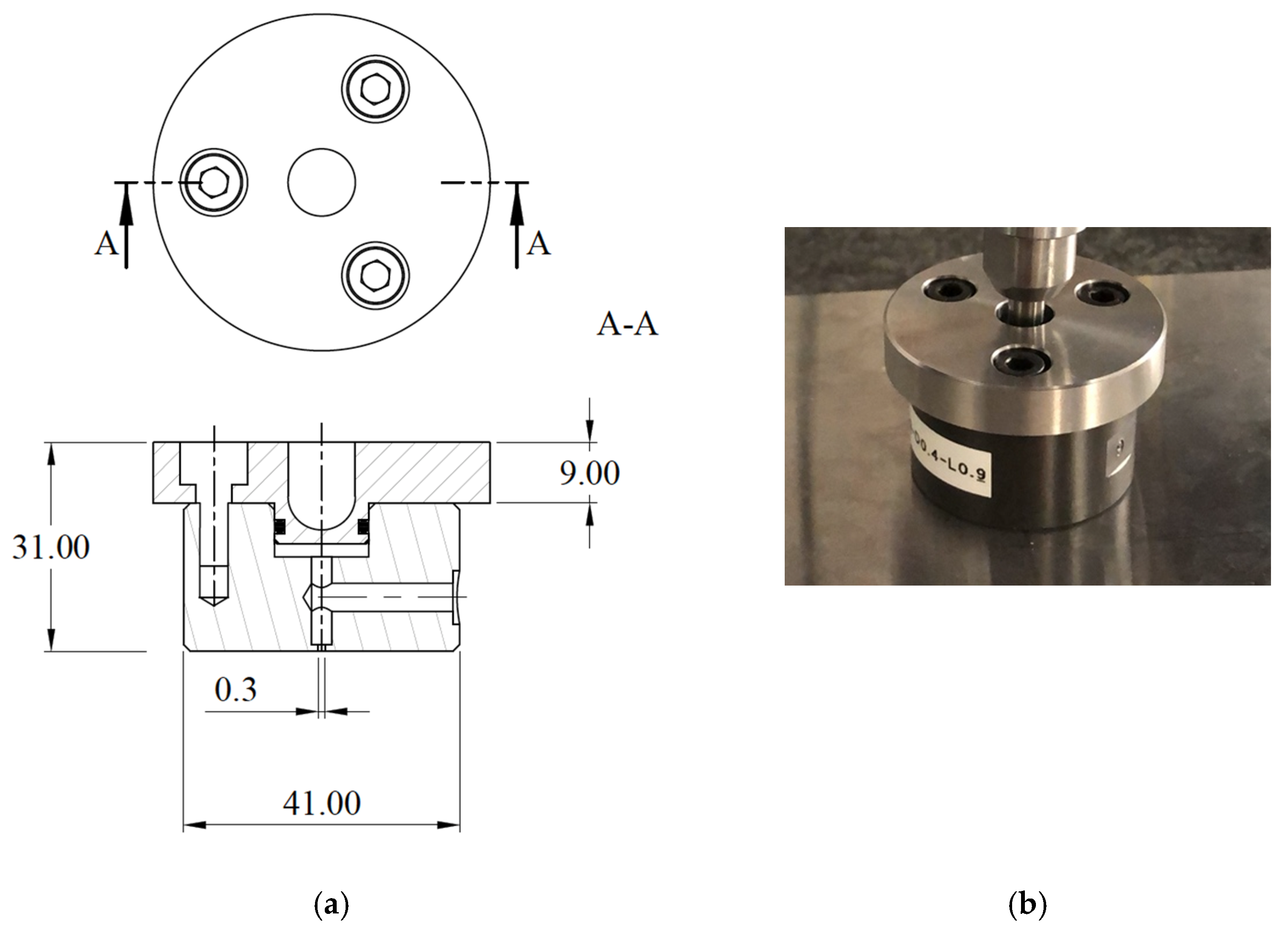
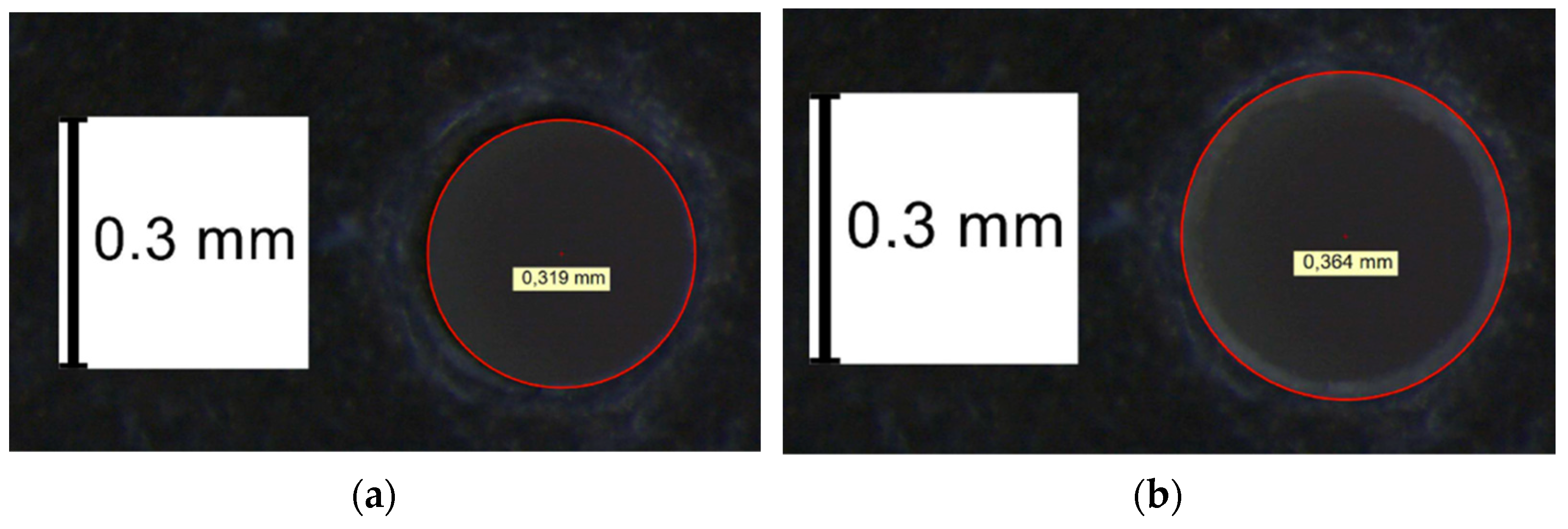
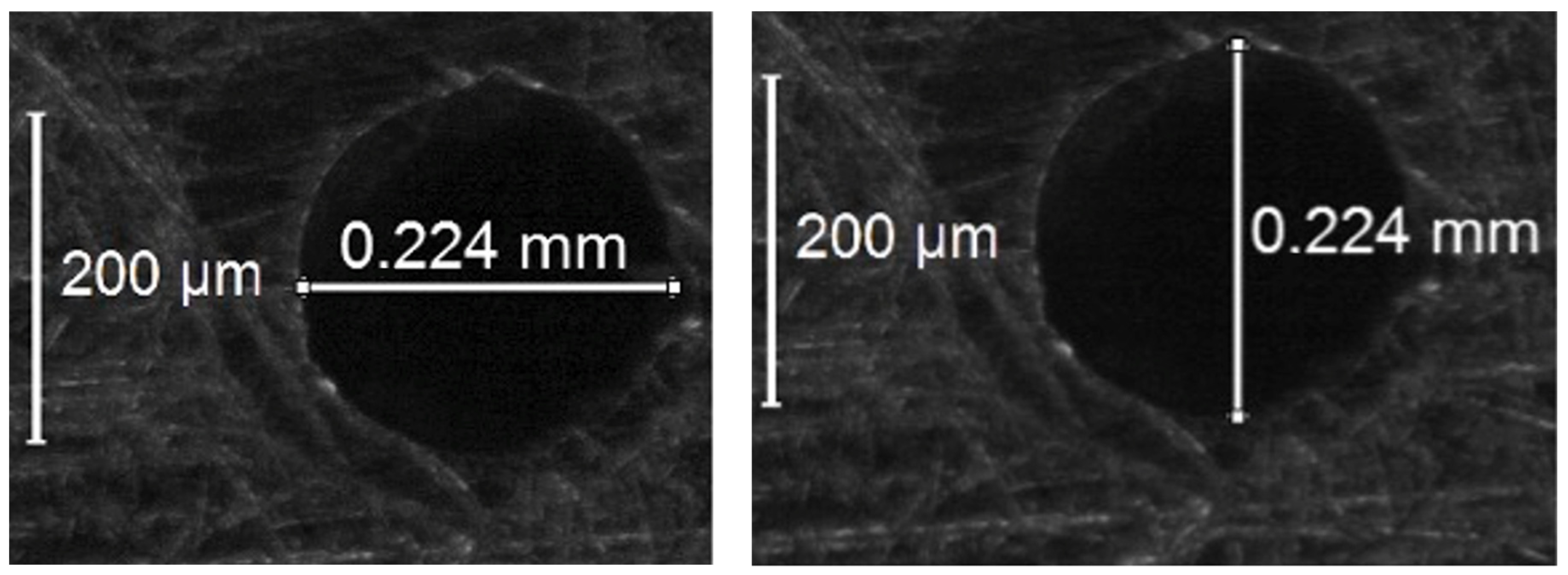
2.1. Pad Geometry
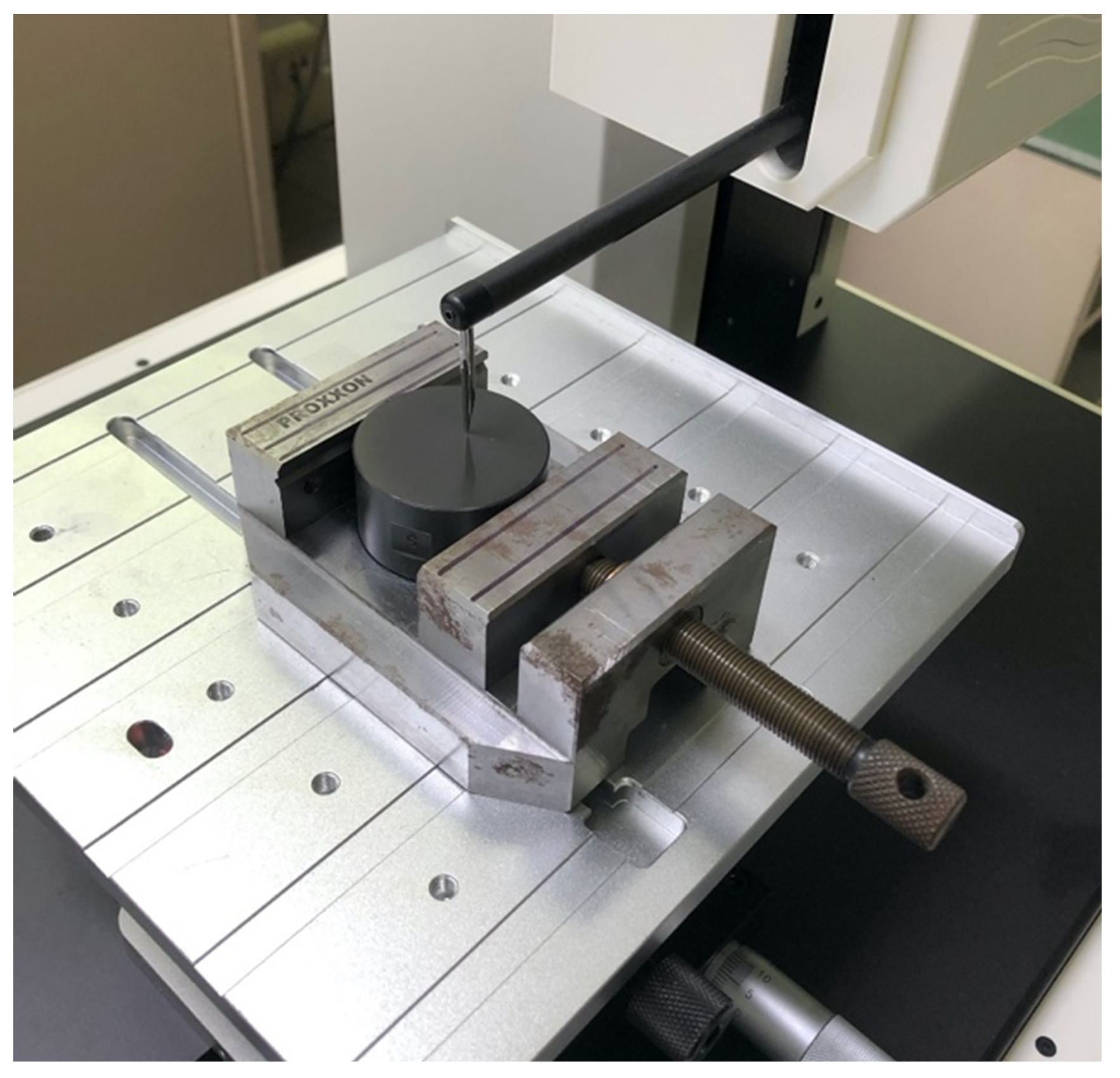
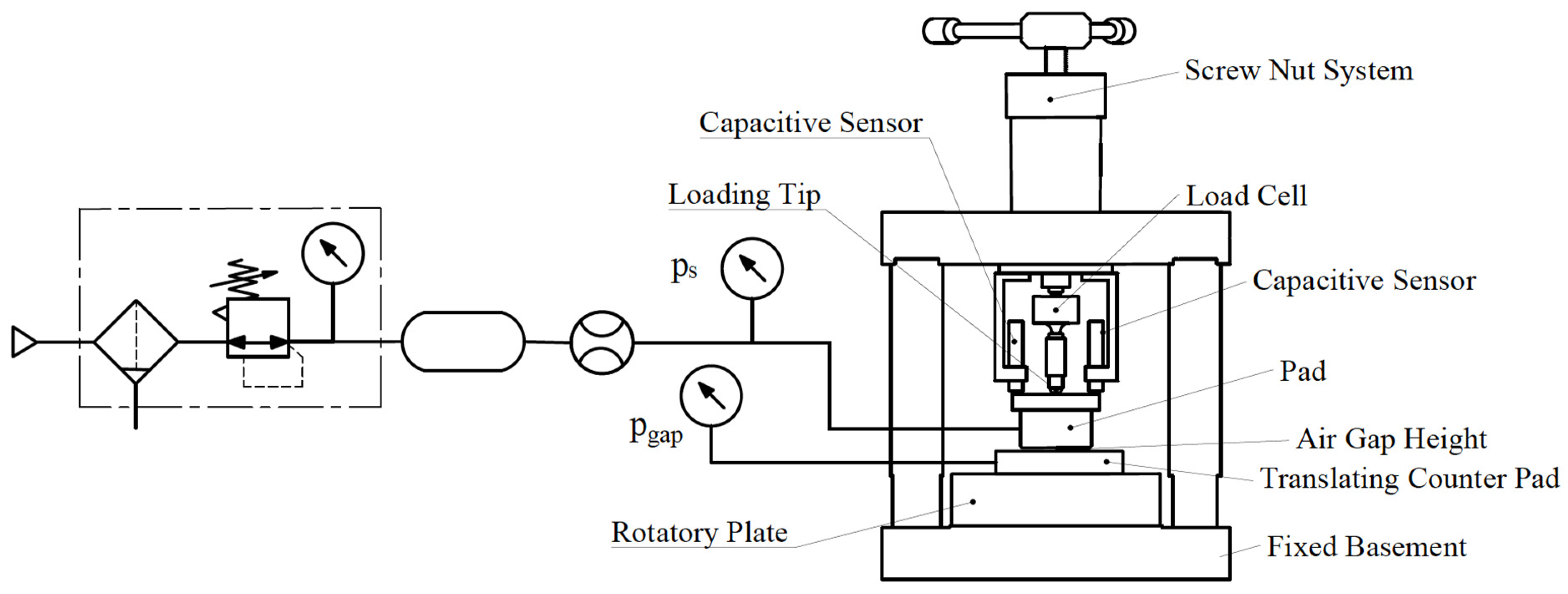
2.2. Test Bench
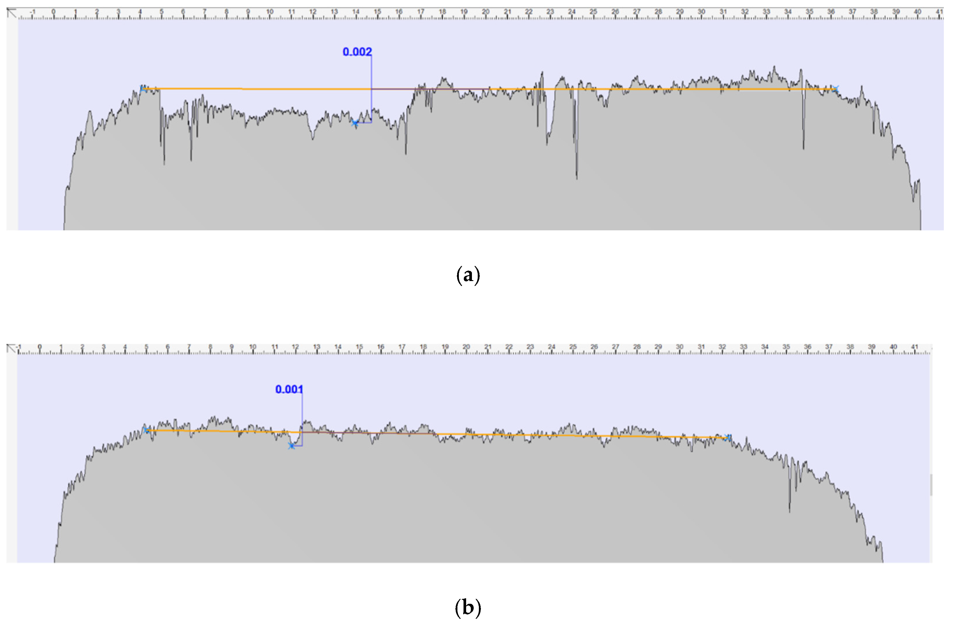
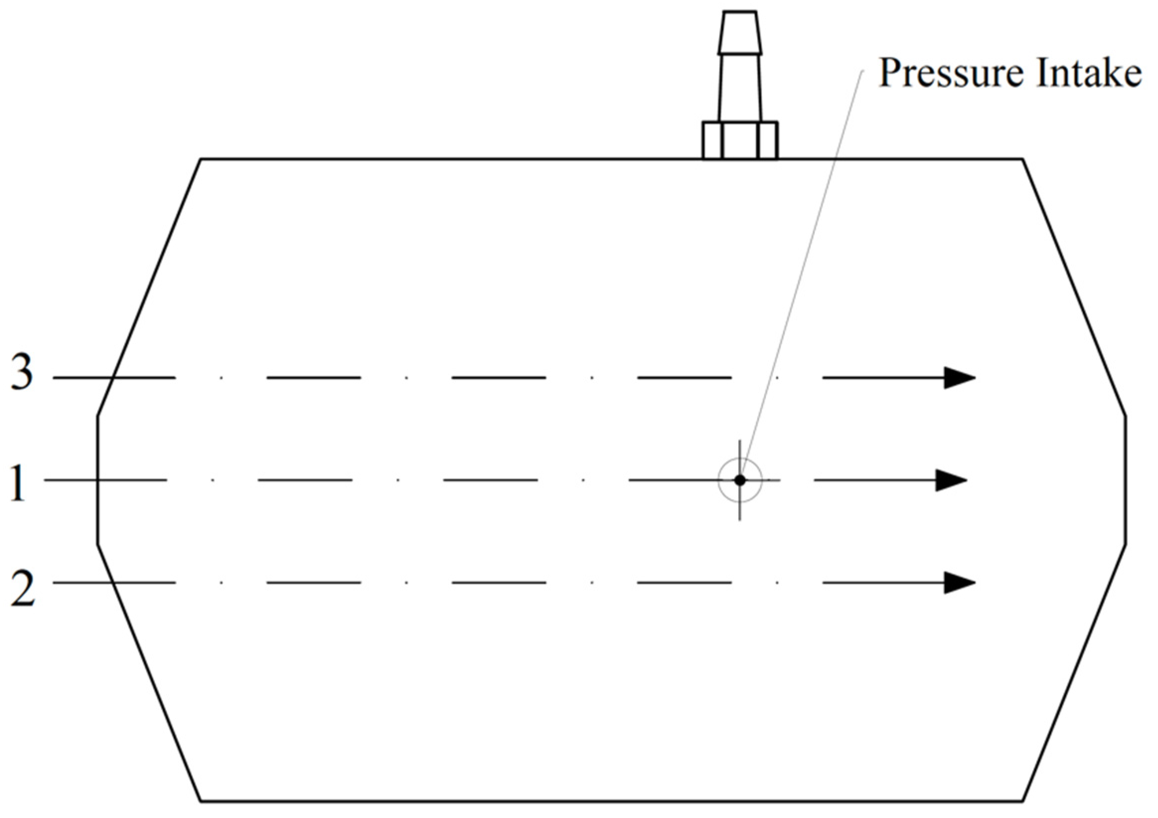
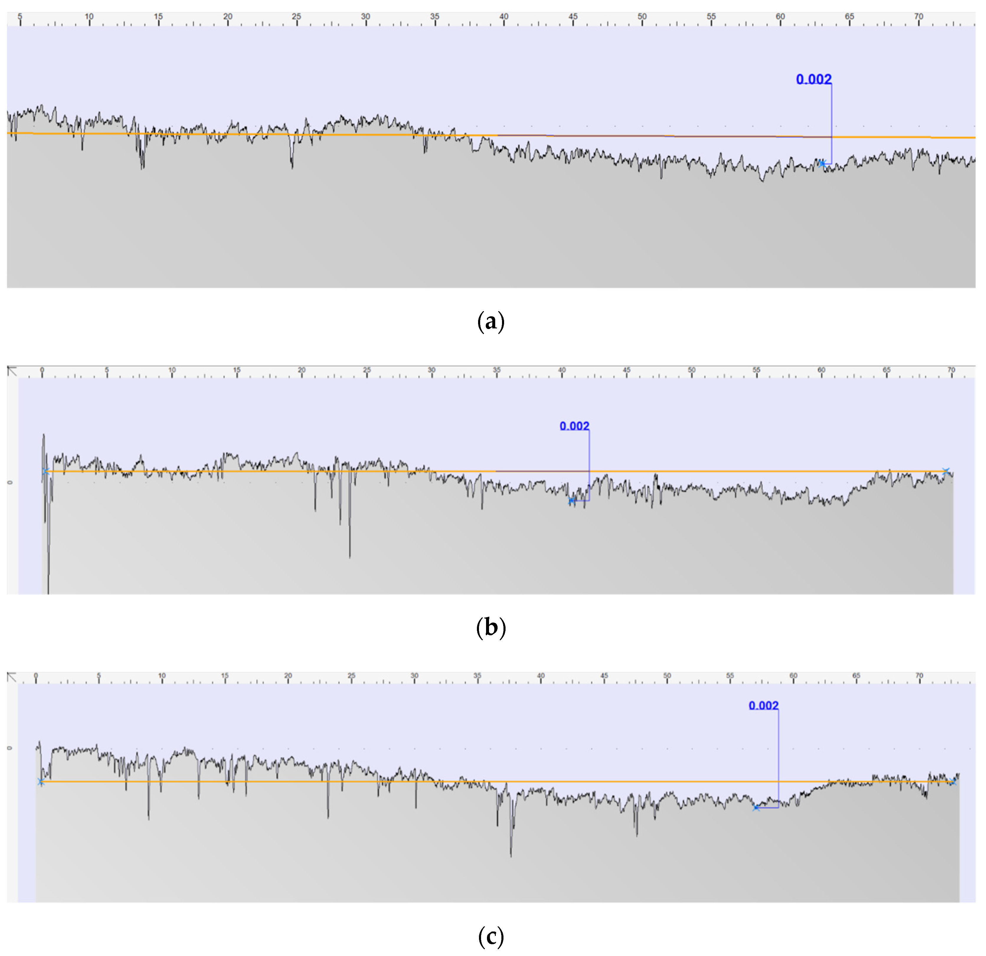
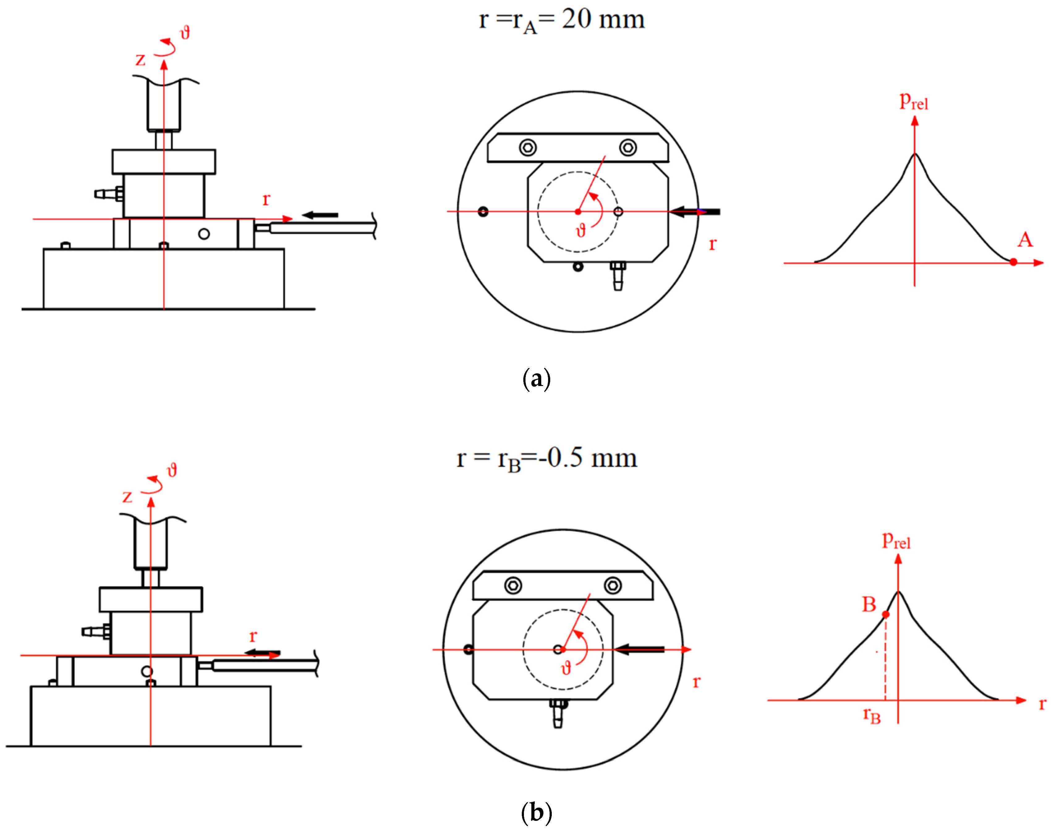
2.3. Pressure Profile Measurements
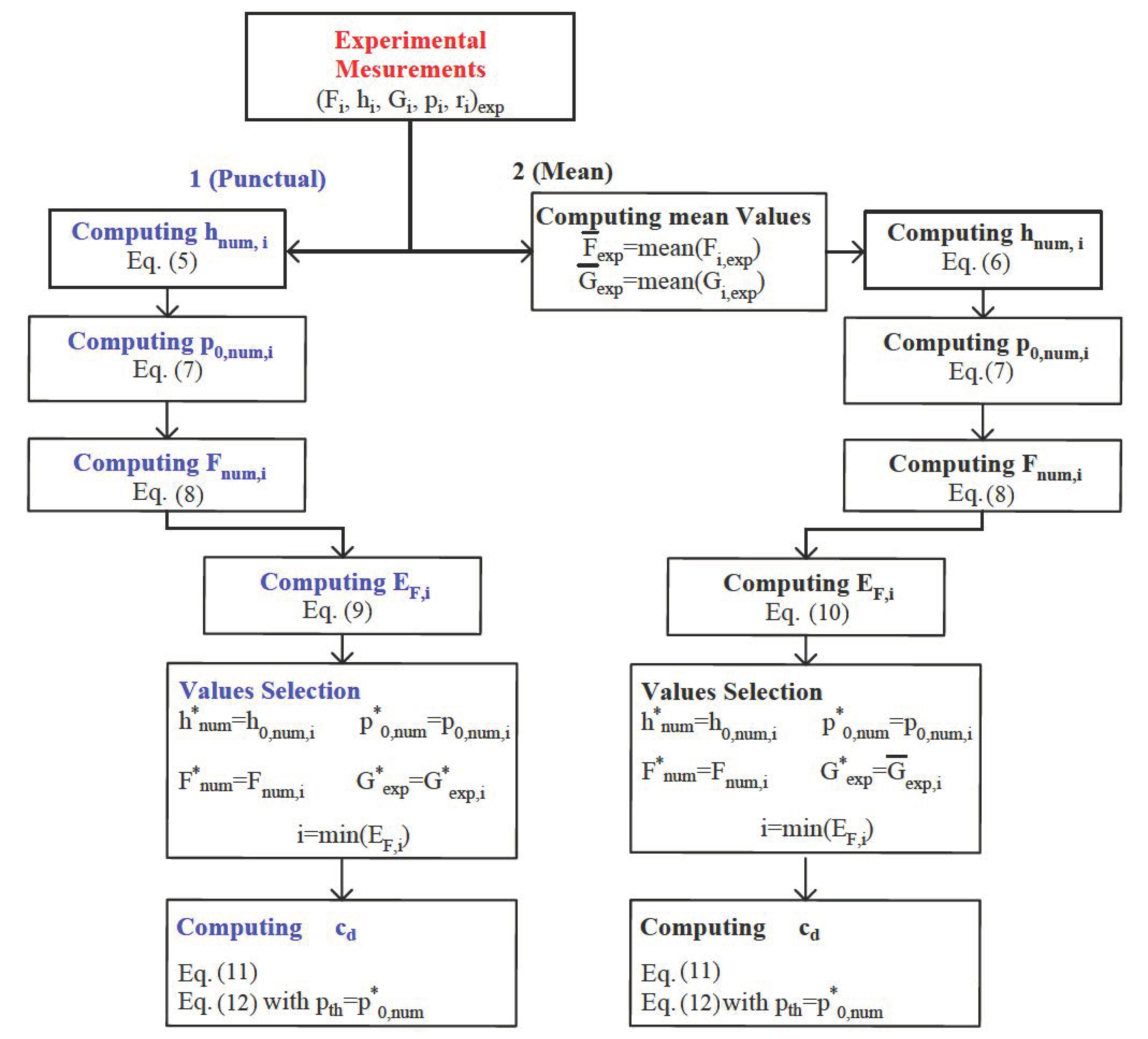
2.4. Static Characterization Procedure
2.5. Identification of the Discharge Coefficients
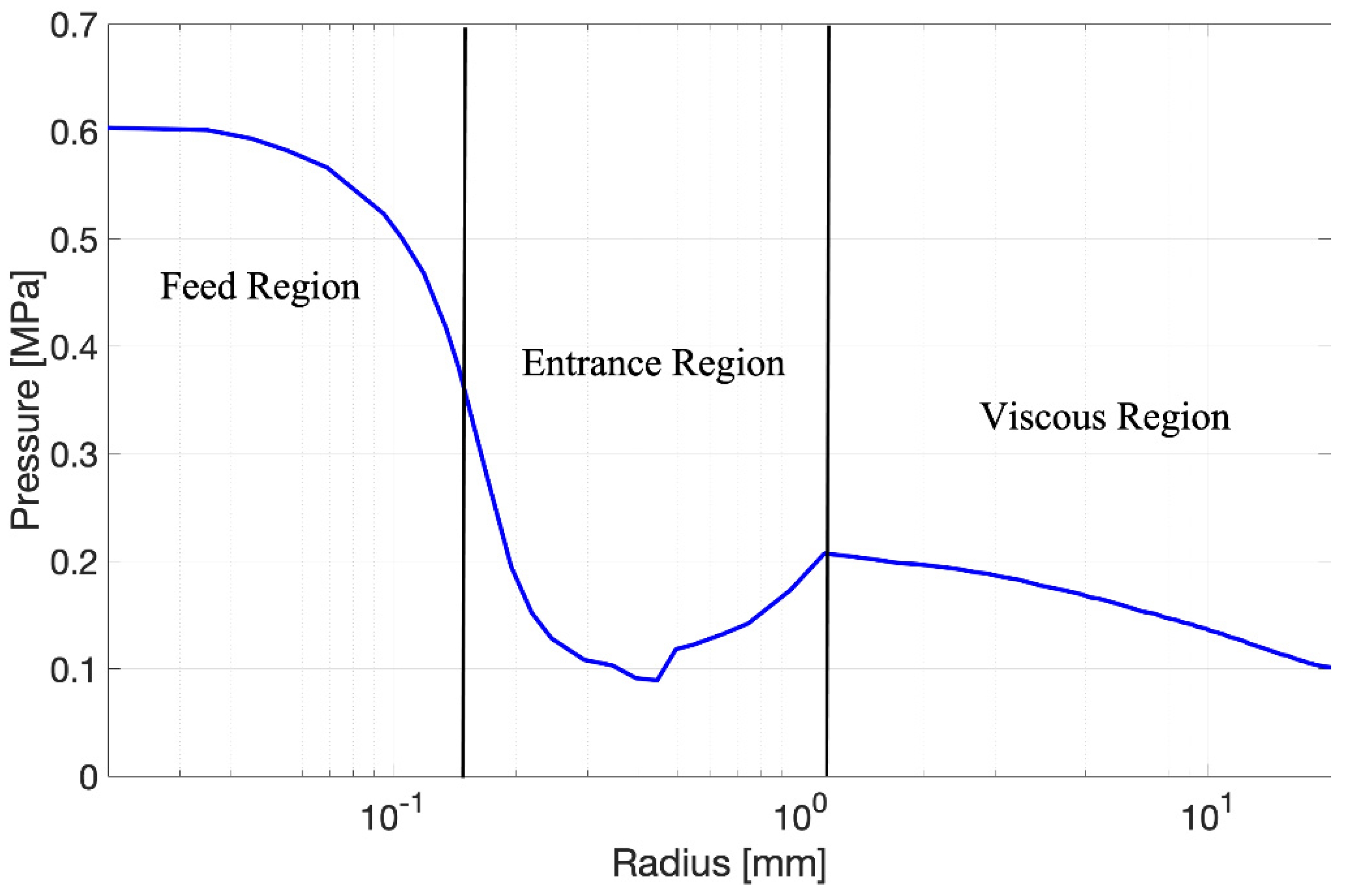
- It is well known that, in aerostatic bearings, the viscous region is by far the largest of the three regions.
- It has been proven numerous times that isothermal and laminar flow models provide accurate predictions in the viscous region [19].
3. Results
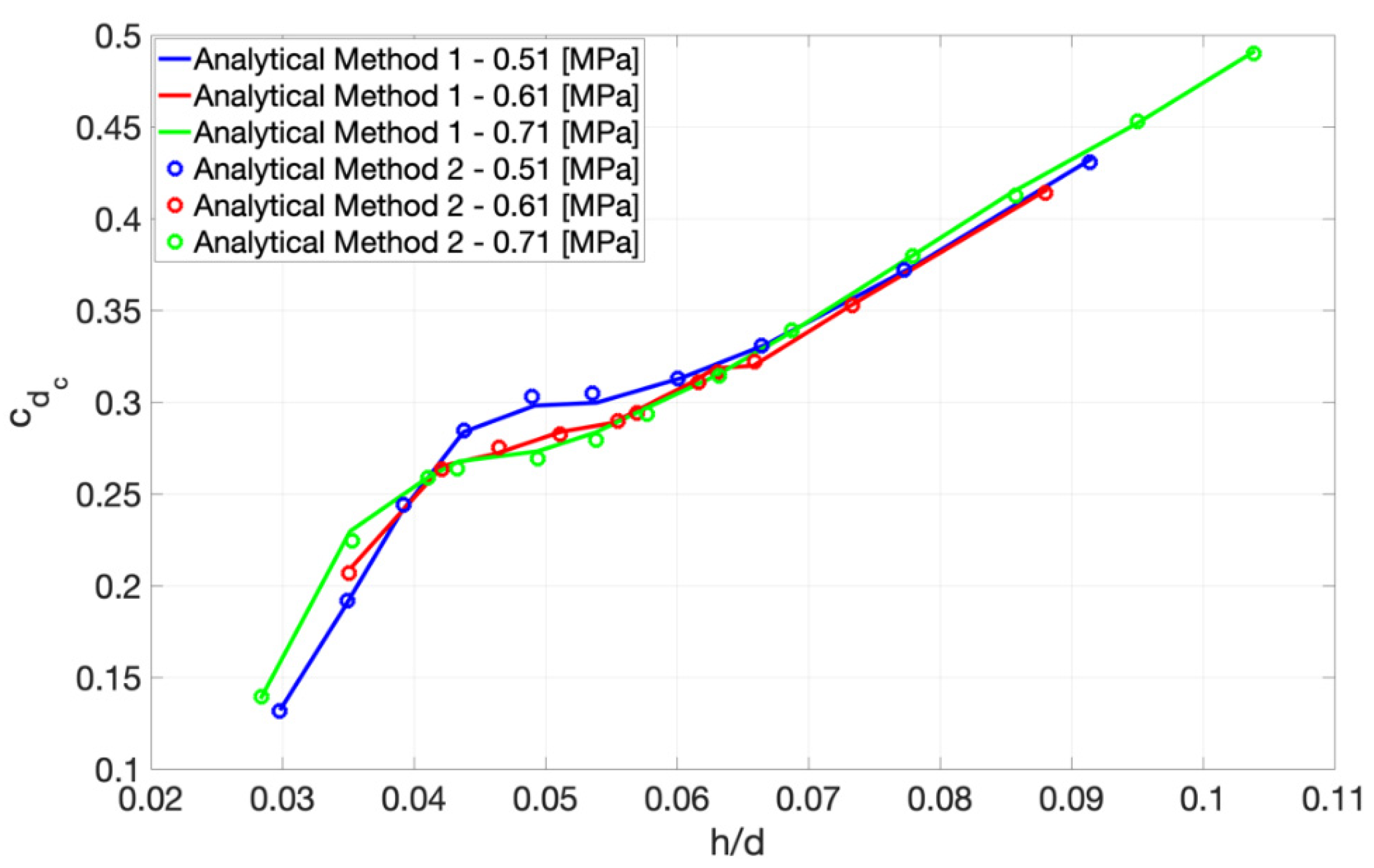
3.1. Discharge Coefficient Identification
3.2. Comparison with Static Characterisation Results
4. Discussion and Conclusions
- Reduce the data scattering thanks to the use of a mathematical framework (closed-form solution).
- Overcome the difficulties related to the evaluation of the air gap height during the acquisition of the pressure profile.
- Minimize the error on the numerical air flow and load capacity.
Author Contributions
Funding
Conflicts of Interest
Appendix A
- isothermal laminar and isoviscous flow
- negligible body forces
- negligible velocity gradients along and
- Newtonian fluid
- constant pressure along the and direction (Due to the axisymmetry of the problem and the small thickness of the air gap.)
- stationary conditions
References
- Lentini, L.; Moradi, M.; Colombo, F. A Historical Review of Gas Lubrication: From Reynolds to Active Compensations. Tribol. Ind. 2018, 40, 165–182. [Google Scholar] [CrossRef] [Green Version]
- Gao, Q.; Chen, W.; Lu, L.; Huo, D.; Cheng, K. Aerostatic bearings design and analysis with the application to precision engineering: State-of-the-art and future perspectives. Tribol. Int. 2019, 135, 1–17. [Google Scholar] [CrossRef]
- Waumans, T.; Al-Bender, F.; Reynaerts, D. A semi-analytical method for the solution of entrance flow effects in inherently restricted aerostatic bearings. In Turbo Expo: Power for Land, Sea, and Air; ASME: Berlin, Germany, 2008; Volume 43154, pp. 1047–1057. [Google Scholar]
- Mori, H.; Miyamatsu, Y. Theoretical flow-models for externally pressurized gas bearings. J. Lubr. Technol. 1969, 91, 181–193. [Google Scholar] [CrossRef]
- Gao, S.; Cheng, K.; Chen, S.; Ding, H.; Fu, H. CFD based investigation on influence of orifice chamber shapes for the design of aerostatic thrust bearings at ultra-high speed spindles. Tribol. Int. 2015, 92, 211–221. [Google Scholar] [CrossRef]
- Zhang, J.; Zou, D.; Ta, N.; Rao, Z. Numerical research of pressure depression in aerostatic thrust bearing with inherent orifice. Tribol. Int. 2018, 123, 385–396. [Google Scholar] [CrossRef]
- Helene, M.; Arghir, M.; Frene, J. Numerical three-dimensional pressure patterns in a recess of a turbulent and compressible hybrid journal bearing. J. Trib. 2003, 125, 301–308. [Google Scholar] [CrossRef]
- Mori, H. A theoretical investigation of pressure depression in externally pressurized gas-lubricated circular thrust bearings. J. Basic Eng. 1961, 83, 201–208. [Google Scholar] [CrossRef]
- Chang, S.H.; Chan, C.W.; Jeng, Y.R. Numerical analysis of discharge coefficients in aerostatic bearings with orifice-type restrictors. Tribol. Int. 2015, 90, 157–163. [Google Scholar] [CrossRef]
- Chang, S.H.; Chan, C.W.; Jeng, Y.-R. Discharge coefficients in aerostatic bearings with inherent orifice-type restrictors. J. Tribol. 2015, 137. [Google Scholar] [CrossRef]
- Miyatake, M.; Yoshimoto, S. Numerical investigation of static and dynamic characteristics of aerostatic thrust bearings with small feed holes. Tribol. Int. 2010, 43, 1353–1359. [Google Scholar] [CrossRef]
- Nishio, U.; Somaya, K.; Yoshimoto, S. Numerical calculation and experimental verification of static and dynamic characteristics of aerostatic thrust bearings with small feedholes. Tribol. Int. 2011, 44, 1790–1795. [Google Scholar] [CrossRef]
- Renn, J.-C.; Hsiao, C.-H. Experimental and CFD study on the mass flow-rate characteristic of gas through orifice-type restrictor in aerostatic bearings. Tribol. Int. 2004, 37, 309–315. [Google Scholar] [CrossRef]
- Al-Bender, F.; Van Brussel, H. A method of “separation of variables” for the solution of laminar boundary-layer equations of narrow-channel flows. J. Tribol. 1992. [Google Scholar] [CrossRef]
- Zhang, J.; Zou, D.; Ta, N.; Rao, Z.; Ding, B. A numerical method for solution of the discharge coefficients in externally pressurized gas bearings with inherent orifice restrictors. Tribol. Int. 2018, 125, 156–168. [Google Scholar] [CrossRef]
- Belforte, G.; Raparelli, T.; Viktorov, V.; Trivella, A. Discharge coefficients of orifice-type restrictor for aerostatic bearings. Tribol. Int. 2007, 40, 512–521. [Google Scholar] [CrossRef]
- Belforte, G.; Colombo, F.; Raparelli, T.; Trivella, A.; Viktorov, V. A new identification method of the supply hole discharge coefficient of gas bearings. Tribol. Des. WIT Trans. Eng. Sci. 2010, 66, 95–105. [Google Scholar]
- Colombo, F.; Lentini, L.; Raparelli, T.; Trivella, A.; Viktorov, V. Dynamic Characterisation of Rectangular Aerostatic Pads with Multiple Inherent Orifices. Tribol. Lett. 2018, 66. [Google Scholar] [CrossRef]
- Belforte, G.; Raparelli, T.; Trivella, A.; Viktorov, V.; Visconte, C. CFD analysis of a simple orifice-type feeding system for aerostatic bearings. Tribol. Lett. 2015, 58, 25. [Google Scholar] [CrossRef] [Green Version]
- Colombo, F.; Lentini, L.; Raparelli, T.; Viktorov, V.; Trivella, A. On the Static Performance of Concave Aerostatic Pads. In IFToMM World Congress on Mechanism and Machine Science; Springer: Cham, Switzerland, 2019; pp. 3919–3928. [Google Scholar]


Publisher’s Note: MDPI stays neutral with regard to jurisdictional claims in published maps and institutional affiliations. |
© 2021 by the authors. Licensee MDPI, Basel, Switzerland. This article is an open access article distributed under the terms and conditions of the Creative Commons Attribution (CC BY) license (https://creativecommons.org/licenses/by/4.0/).
Share and Cite
Colombo, F.; Lentini, L.; Raparelli, T.; Trivella, A.; Viktorov, V. An Identification Method for Orifice-Type Restrictors Based on the Closed-Form Solution of Reynolds Equation. Lubricants 2021, 9, 55. https://0-doi-org.brum.beds.ac.uk/10.3390/lubricants9050055
Colombo F, Lentini L, Raparelli T, Trivella A, Viktorov V. An Identification Method for Orifice-Type Restrictors Based on the Closed-Form Solution of Reynolds Equation. Lubricants. 2021; 9(5):55. https://0-doi-org.brum.beds.ac.uk/10.3390/lubricants9050055
Chicago/Turabian StyleColombo, Federico, Luigi Lentini, Terenziano Raparelli, Andrea Trivella, and Vladimir Viktorov. 2021. "An Identification Method for Orifice-Type Restrictors Based on the Closed-Form Solution of Reynolds Equation" Lubricants 9, no. 5: 55. https://0-doi-org.brum.beds.ac.uk/10.3390/lubricants9050055