Towards Ecological Alternatives in Bearing Lubrication


1
LGMM Laboratory, Faculty of Technology, 20 août 1955 University-Skikda, Skikda 21000, Algeria
2
Université de Lyon, CNRS INSA-Lyon, LaMCoS, UMR5259, F-69621 Villeurbanne, France
3
Department of Mechanical, Aerospace, and Nuclear Engineering Rensselaer Polytechnic Institute, Troy, NY 12180-3590, USA
*
Author to whom correspondence should be addressed.
Lubricants 2021, 9(6), 62; https://0-doi-org.brum.beds.ac.uk/10.3390/lubricants9060062
Submission received: 8 May 2021
/
Revised: 1 June 2021
/
Accepted: 1 June 2021
/
Published: 9 June 2021
(This article belongs to the Special Issue Research Trends in Hydrodynamic Journal and Thrust Bearings)
Abstract
:Hydrogen is the cleanest fuel available because its combustion product is water. The internal combustion engine can, in principle and without significant modifications, run on hydrogen to produce mechanical energy. Regarding the technological solution leading to compact engines, a question to ask is the following: Can combustion engine systems be lubricated with hydrogen? In general, since many applications such as in turbomachines, is it possible to use the surrounding gas as a lubricant? In this paper, journal bearings global parameters are calculated and compared for steady state and dynamic conditions for different gas constituents such as air, pentafluoropropane, helium and hydrogen. Such a bearing may be promising as an ecological alternative to liquid lubrication.
1. Introduction
Hydrogen is the cleanest fuel available as its combustion product is water. This advantage has enabled hydrogen technology to quickly establish itself as the technology of the future not only for fuel cell vehicles (FCVs), but also for other high-energy consumption applications. Combining a hydrogen fuel cell with an electric motor is obviously an ideal situation for obtaining mechanical energy without emitting greenhouse gases or other forms of pollution. The hopes of commercialization seem hypothetical in the short to medium term, thus a credible transitional solution has emerged by decoupling the following two “futuristic” technologies considered: hydrogen on the one hand, and the fuel cell on the other. Therefore, we propose as a first step to use hydrogen with a mature technology, namely, the internal combustion engine and its bearing components.
The internal combustion engine can, in principle and without significant modifications, run on hydrogen to produce mechanical energy by releasing only water vapor and oxides of nitrogen (NOx). As a result, the hydrogen internal combustion engine could contribute to meeting the following double challenge already identified: remedying the scarcity of oil resources and reducing greenhouse gas emissions, provided, of course, the hydrogen used is not made from fossil fuels. Converting such an engine to hydrogen does not change its basic functioning, only a few modifications become necessary. The specific power limitation can be eliminated via appropriate injection devices (high-pressure direct injection) and supercharging (turbo or compressor). We can then end up with extremely high-efficiency engines (greater than 40%) over the entire operating range. Such efficiencies can even exceed those of the best diesel engines. Concerning the technological solution leading to the compact engines, questions to be asked are as follows: Is it possible to use hydrogen both as a fuel and as a lubricant? Can systems in the combustion engine be lubricated with hydrogen?
In the context of the increased evolution of mechanical systems, the constant development of vehicle propulsion also leads to an improvement in fuels and lubricants (brake fluid, refrigerant, or engine oils). In the development of fuels and lubricants, increased propulsion performance and efficiency play a crucial role, but protecting the driveline from wear and deposits is also important. In the age of global warming, protecting the environment is becoming increasingly important. It is therefore logical that efforts to increase energy efficiency also target a more economical use of the available resources. The search for new alternative fuels is thus one of the central missions in advancing the technology. To develop fuels and lubricants that are environmentally compatible is particularly important, whether at the stage of their manufacture, disposal, or from the point of view of their biodegradability.
On the other hand, the energy sources used for road transportation include natural gas (CNG and LNG), biogas, liquid gas (LPG), bioethanol, biodiesel, hydrogen (H2), and electricity, among others. Only biogas, bioethanol, and biodiesel, as well as hydrogen, wind, solar or hydroelectricity, constitute complete ecological alternatives. Natural gas and liquid gas are indeed still fossil energy sources (i.e., non-renewable). However, they allow combustion that is less polluting than gasoline and diesel. In addition, their ecological balance can be significantly improved with the addition of biofuels. As for hydrogen propulsions—whether it is a combustion engine, a gas turbine, or a fuel cell—the significant energy expenditure required to produce and transport hydrogen is affecting their otherwise very good ecological balance.
Ammonia refrigeration lubricant is specifically designed for use in ammonia refrigeration systems. Ammonia refrigeration lubricant (R717AC-LT) is highly stable and specifically formulated so that it does not react with ammonia. The technology is also used by most original equipment manufacturers for their factory and service fill. These lubricants have very low volatility, enhanced stability, and reduced solubility in ammonia, resulting in very low lubricant use and increased efficiency of the ammonia refrigeration system. The refrigerants R717AC-LT and R717AC-XLT are formulated to have even better low-temperature properties and are designed to operate in extremely low-temperature flash freezers.
If the combustion gas and lubricating gas are the same, a separate lubricant feeding system becomes unnecessary. A realistic solution in a hydrogen or refrigerant environment is a lubrication system using one of these as the working fluid. A number of studies over the last 20 years have shown that bearings are the best options for a consequent range of applications, such as oil-free turbomachinery [1,2]. To implement bearings into new systems, many problems remain. Studies already exist, but they are either experimental [3] or analytical without a specific lubricant behavior analysis [4]. Gas-lubricated bearings require a specific thermo-hydro-dynamic (THD) or thermo-elasto-hydro-dynamic (TEHD) theoretical and numerical model. In this paper, we investigate both the static and dynamic bearing behavior when running with hydrogen or refrigerating gas. A TEHD approach is used with a gas constitutive equation to describe pressure, density, viscosity, and temperature. A GRE (generalized Reynolds equation) for turbulent flow, a nonlinear cubic EoS (equation of state) for two-phase flow, a 3D turbulent, thin-film energy equation, and three-dimensional (3D) thermal equations in solids are all needed. Journal bearings global parameters are calculated and compared for steady state and dynamic conditions for different gas constituents.
There are no available experimental studies in the literature to which the present results can be meaningfully compared. Indeed, experiments with local behavior (of, say, pressure, temperature and density) are extremely rare for any type of gas bearing, but particularly in the case of such a specific geometrical configuration. There are dozens of parameters that can significantly influence the behavior, so the present study must be considered as preliminary, rather than definitive and exhaustive.
There are numerous recent papers on the influence of tribology on the environment, which have spawned a movement with various names such as “green tribology”, “environmentally friendly” lubricants, etc. Most of such articles take the form of finding biodegradable lubricants [5,6], minimizing the use of lubricants through alternate techniques [7], deriving plant-based lubricants [8], and others. There is much less research dedicated to this theme using gaseous lubricants such as air or cryogenics. A literature search on this topic unearthed very few papers, one of the few being Ref. [9]. Our current paper seeks to begin to partially fill this void by applying a basic analysis to the widely used three-lobe gas bearing with feeding grooves, as a candidate for application with benign gaseous lubricants.
2. Equation of State and Vapor/Liquid Transition
When the pressure is sufficiently close to the vapor pressure, the assumption of the ideal gas theory used for compressible gas behavior (density is dependent on pressure and temperature) frequently is inadequate. The existence of two-phase flow has been shown experimentally under specific conditions, e.g., when refrigerant is introduced into the GFB lubrication system. The use of a nonlinear EoS (equation of state) capable of describing the variation in density as a function of pressure and temperature, and of the vapor/liquid transition, is necessary. Since density and pressure are strongly coupled, the GRE and EoS must be solved simultaneously. Viscosity is also related to temperature and the fraction of liquid in the fluid. We have chosen a modified Peng–Robinson EoS [10], with a dimensional formulation written as follows:
with:
where p is the pressure, R the ideal gas constant, T the local temperature, B and mρ are EoS constant coefficients, whereas aρ is an EoS temperature-dependent coefficient.
The molar mass M, the critical pressure pc, the critical temperature Tc and the acentric factor ωρ are among the fluid characteristics that can be found in a fluid database. The primary inaccuracy of the EoS prediction is due to a poor evaluation of the vapor pressure at which the transition occurs. To overcome this, we use the Clapeyron formula to predict the vapor/liquid transition. From the Dupré approximation, three couples (Ti, psat (Ti)) are needed (for a given gas) to predict the vapor pressure at any given temperature [11], as follows:
where C1, C2, C3 are three phenomenological constants (for a given gas). These three couples can easily be found in the literature for a large group of fluids.
3. The Vapor/Liquid Transition Phase
The vapor to liquid phase may occur for some lubricants. The vapor/liquid transition model we choose has shown good efficiency in previous works [12]. A continuous sinusoidal transition, which is a function of the local pressure, the vapor pressure and the minimum speed of sound cmin in the mixture, predicts accurate equivalent parameters for the mixture. The subscript l is for the value of a given parameter for the liquid phase, and v for the vapor phase. This transition occurs for the three parameters of density ρ, thermal conductivity k and molecular viscosity µ. We can obtain the pressure from the vapor pressure psat to its upper limit psat + Δp for which the fluid equivalent parameters are calculated as follows:
and the following:
Noting that cmin is the minimal speed of sound in the vapor phase [13] calculated from pressure, density, and the adiabatic index γ for an ideal isentropic gas. The latter is assumed to be 7/5, as is the case for the diatomic molecules from the kinetic theory.
4. Generalized Reynolds Equation
In this section, we present a generalized Reynolds equation (GRE) [14], which describes the pressure field in the lubricant under thin-film assumption. The pressure field in the bearings is obtained by solving the steady-state GRE (6) for turbulent, compressible fluids with variable viscosity across the film thickness. It can be written in its nondimensional form as follows:
with the following:
where the following applies:
Boundary conditions for pressure are based on an imposed pressure at both ends and in the supply groove if any. Our model ensures the continuity for physical values, such as density and viscosity, for the vapor/liquid transition. We also take into account in this GRE the turbulent flow effects due to an equivalent viscosity term, which combines the molecular viscosity and the eddy viscosity due to turbulent flow [15].
The transition between the laminar and turbulent regime for the bearings is considered. Different regimes can exist at different locations inside the bearing. When the local Taylor number TaL reaches the value Tac, the limit between the laminar flow and Taylor vortex regimes is reached with the following:
and the following:
The critical Taylor number Tac is taken from the empirical relation given in [16]. The value 41.2 comes from the theory of the Taylor vortices and is the limiting value when the eccentricity ratio εi is zero. When TaL reaches 2Tac, the flow becomes turbulent.
5. Energy Equation
This section shows how we consider the THD effects in our model, and is related to the lubricant thermodynamic behavior. We solve a steady-state 3D turbulent thin-film energy equation (Equation (8)) to obtain a local thermal field (and local temperature-dependent molecular viscosity). It can be written in its non-dimensional form as follows [15]:
with the following:
where the following applies:
The thermal model accounts for 3D (circumferential, radial and axial) temperature variations. The thermal expansion coefficient must be determined to solve the equation. It is obtained using the ideal gas law. It leads to the following expression in the vapor phase:
The thermal expansion coefficient is considered to be zero in the liquid phase. The assumption of an ideal gas should be valid for several reasons, among them being that the ideal gas law gives a very good approximation far from the vapor pressure value. In addition, when close to the transition and in the transition, the compressibility terms become less important in magnitude, since the lubricant tends to liquid behavior.
6. Three-Dimensional Eddy Viscosity Model
We need a zero-equation turbulent model that gives the eddy viscosity as a 3D function of the local fluid parameters, and can also be used in a THD model. We choose a 3D eddy viscosity model in which the influence of turbulence is calculated through a modified version of the Reichardt empirical law.
The empirical coefficients are based on shear stress and velocity measurements in a pipe flow [17], and are adapted to fit the experimental data [18]. In that case, the eddy viscosity is given by the following formula:
with the following:
where κ = 0.4 is the Von Karman constant, δL = 10.7 is the thickness of the laminar sublayer and y+ is the dimensionless distance from the wall.
7. Turbulent Conduction
The conductive term in the energy equation corresponds to the heat transfer due to the conductivity of the fluid. When in the laminar regime, the conductivity is an intrinsic fluid property and the conductive heat transfer is the result of the mean temperature gradient. In the turbulent regime, the fluctuating velocity generates an extra heat transfer. Therefore, the turbulent conductive term can be written as the sum of the laminar and turbulent conductive terms and again k* = k + kt.
with the following:
where αf is the heat transfer diffusivity, as follows:
The turbulent Prandtl number Prt is the ratio between the momentum eddy diffusivity and the heat transfer eddy diffusivity. Following the Reynolds analogy, it is often assumed in lubrication that Prt = 1 [19].
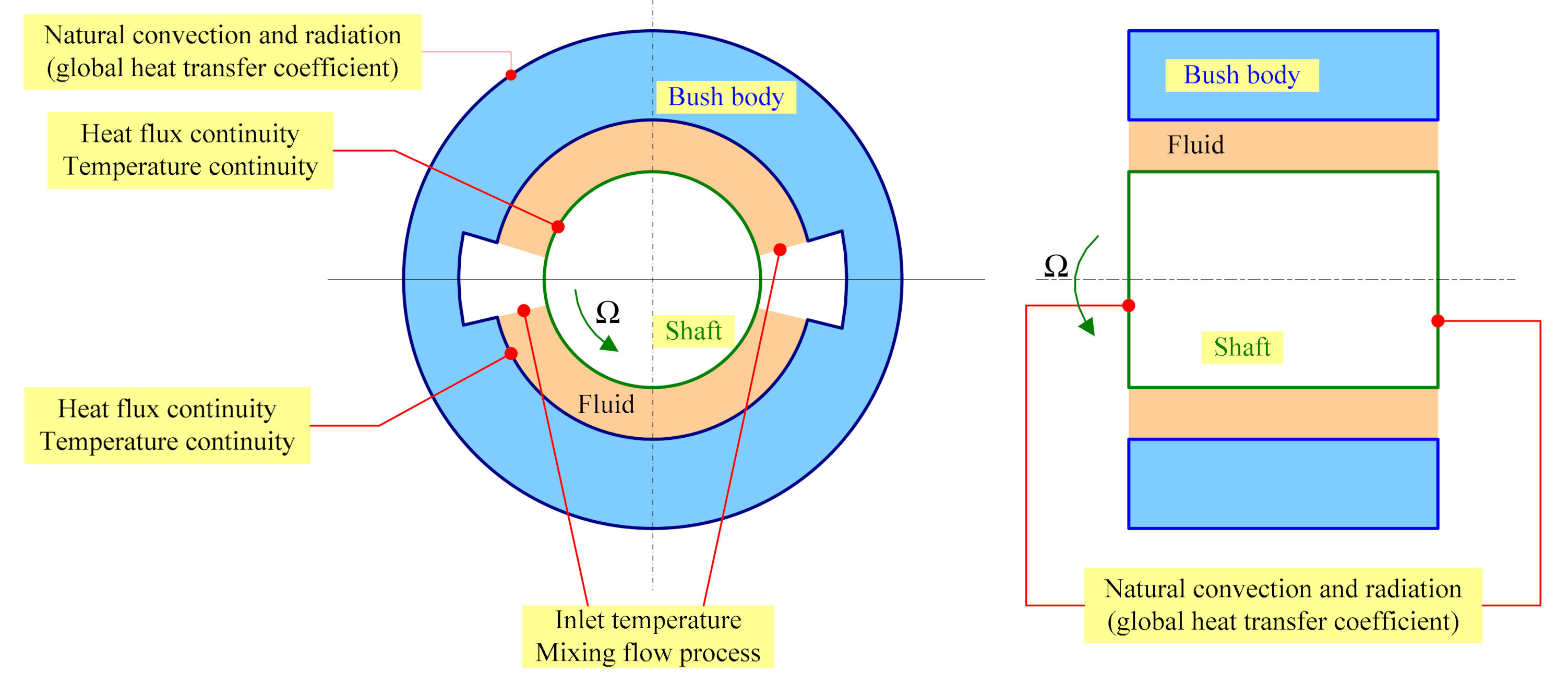
8. Thermal Behavior of the Solids
The temperature generated in the fluid flows through the solids, as shown in Figure 1. For simplicity and demonstration purposes, a two-lobed bearing is shown. In agreement with the experimental results of Dowson et al. [20], it can be assumed that the temperature Ts of the fast-rotating shaft is independent of the coordinate angle θ, and in these conditions, the heat equation becomes the following:
with the following:
To obtain the temperature Th in the bush, we neglect the axial gradient of the temperature. Therefore, the heat equation can be written as follows:
with the following:
The temperature boundary conditions are the following:
8.1. Film–Housing Interface
8.2. Housing–Air Interface
The housing external surface is in contact with the surrounding air. The thermal exchange is mainly due to convection and radiation. We combine these two phenomena using a global coefficient of exchange hh, and we can write the following at the external surface:
which can be written in dimensionless form, as follows:
8.3. Film–Shaft Interface
8.4. Shaft–Air Interface
At this location we can write the following:
thus, the following applies:
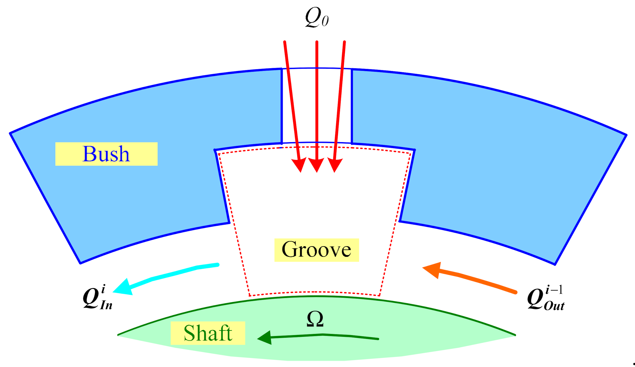
8.5. At the Entry of the Film
There is a mixing flow process at the entry of each sector (see Figure 2). The present approach applied to the grooves and sectors is rather simple and straightforward, consistent with the aims of the paper. A much more sophisticated study on the topic is due to Xie et al. [23] using CFD on an individual groove, but its results would be difficult to apply to this paper.
The following flows are involved:
at the entry of sector i
at the exit of sector i
in the axial direction
Thus, the temperature at the entry is given by the following:
where λ is a mixing coefficient depending on the operating conditions [24].
9. Viscosity Variations
Temperature variations have a direct impact on lubricant viscosity. For gas, we use the following explicit formulation, which gives the molecular viscosity as a function of the temperature [25]:
The Sutherland number Su is a constant that depends on the lubricant composition, and whose value can be found in the literature.
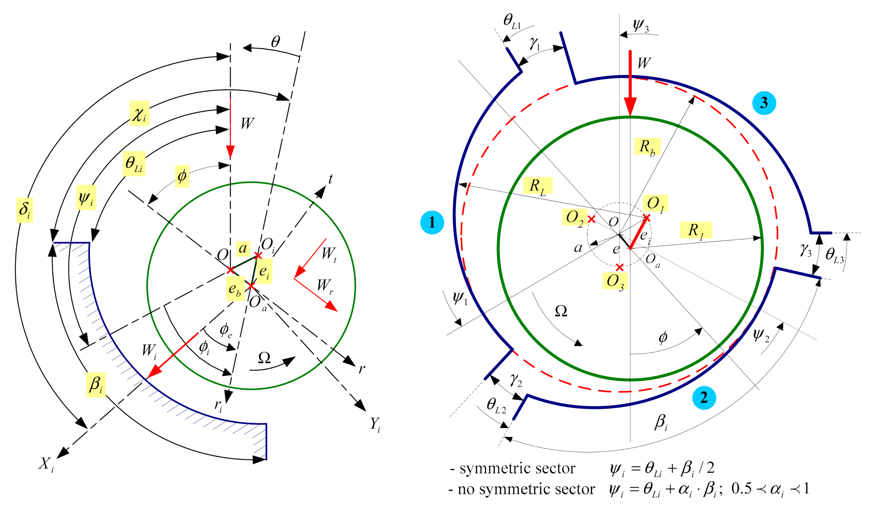
10. Bearing Geometry
A sketch of the three-lobed bearing for which the calculations are performed is given in Figure 3. The dimensionless film thickness is as follows:
The subscript i represents the lobe 1, 2, or 3. The circumferential origin (θ = 0) of each lobe (used for the local film thickness determination in the calculations) is defined by the lobe line-of-centers as shown on the left. The bearing global circumferential origin (θb = 0) is defined by the bearing line-of-centers, the dash/dot line, on the right-hand figure.
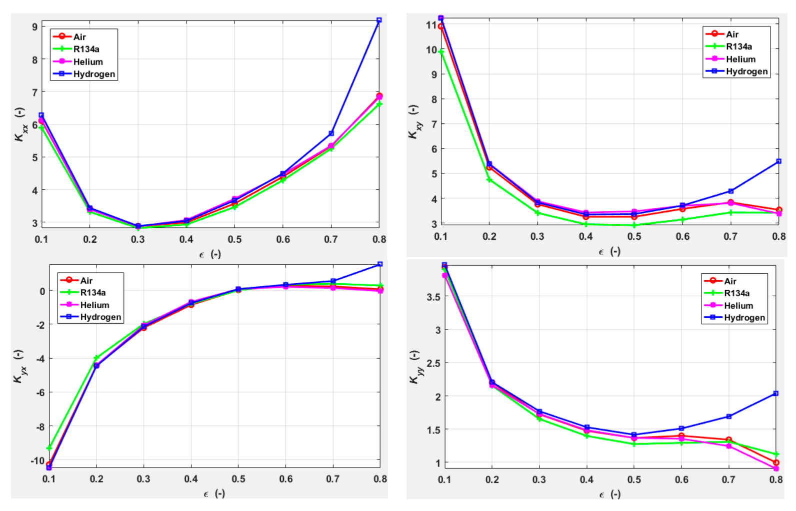
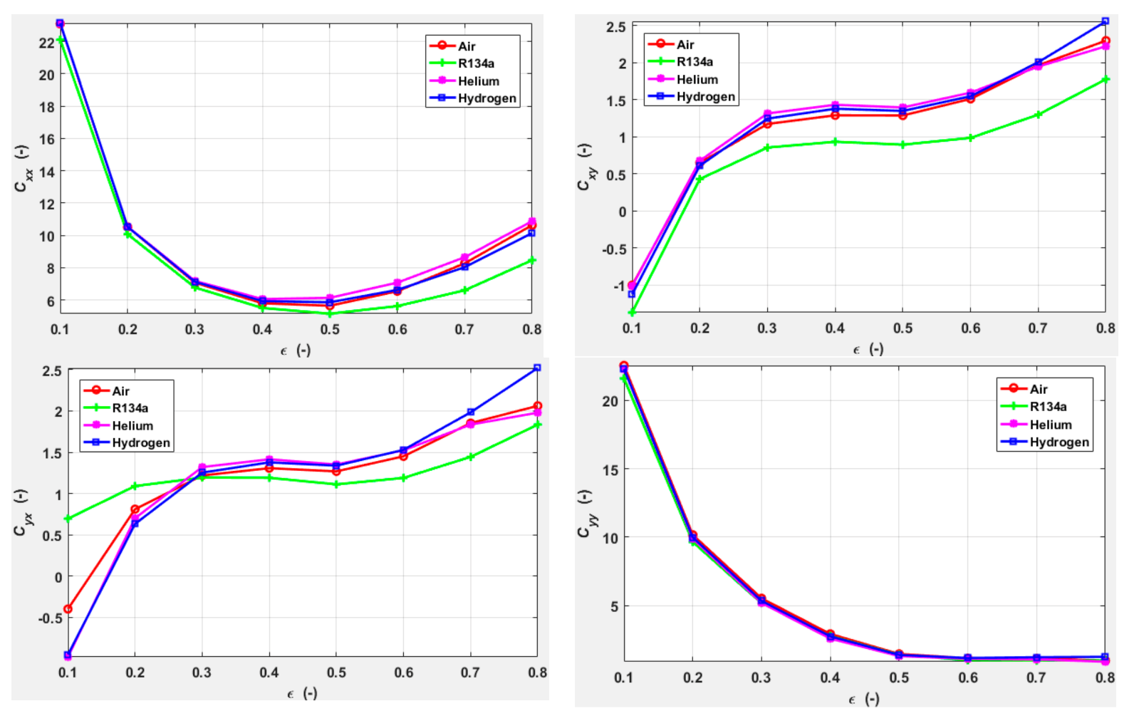
11. Dynamic Coefficients
The expression of fluid film forces in the radial and tangential directions (ri, ti) is given in Appendix A. From these forces, and for each sector, the stiffness and damping coefficient can be obtained, as follows:
The first matrix describes the oil-film response to shaft perturbation in displacement, and is the (non-dimensional) stiffness matrix . The second matrix describes the response to shaft velocity perturbation, and is the (non-dimensional) damping matrix .
The relationship between the coefficients in the (ri, ti) coordinates to expressed in the coordinate system (Xi, Yi) is easily determined by the following:
where the rotation matrix for each sector [Ri] is defined as the following:
Finally, the global stiffness and damping matrices can be given in the coordinate system (x, y) using the rotation matrix [Q], and can be obtained by summing each matrix for each sector. Thus we have the following:
The rotation matrix [Qi] is defined as follows:
with the following dimensionless variable definition:
12. Finite Difference Method
The continuous fluid model produces partial differential equations (PDEs) that depend on both time and space. There is no analytical solution to the set of coupled governing equations. Instead, we use spatial discretization schemes to transform such PDEs into algebraic systems that deliver approximate solutions. Among the different classes of available approaches, e.g., the finite element method (FEM), finite volume method (FVM), or finite difference method (FDM), the selected FDM provides the greatest flexibility when facing non-standard PDEs. The FDM has been one of the first methods used for solving hydrodynamic lubrication problems. The FDM theory is based on simple principles, but it can solve rather complex TEHD problems in an efficient and accurate way. Therefore, many recent studies use the FDM to solve hydrodynamic or TEHD problems [21,22]. In addition, there is no doubt that the FDM is convenient when working with simple geometries such as the plain journal bearing. The number of circumferential points in each lobe is 60, the number of axial points is 11, and the number of radial points is 11.
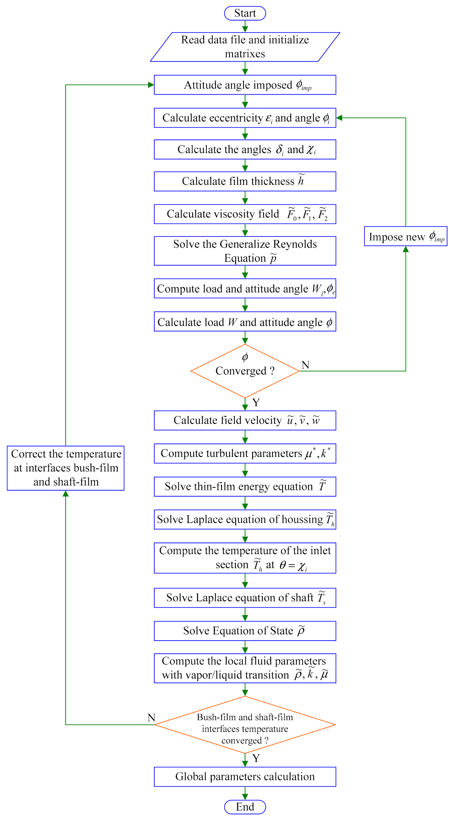
A flow chart of the computations is provided in Appendix C.
13. Results and Discussion: 3D THD Analysis
We use a journal bearing whose characteristics and operating conditions are described in Table 1. The global heat transfer coefficients from the shaft surface in the radial and axial directions, for lack of specific information, are assumed equal. Although we did not perform sensitivity tests as to the overall heat transfer coefficients, the computed results seem internally consistent.
Lubricant properties are given in the following Table 2.
Static Characteristics
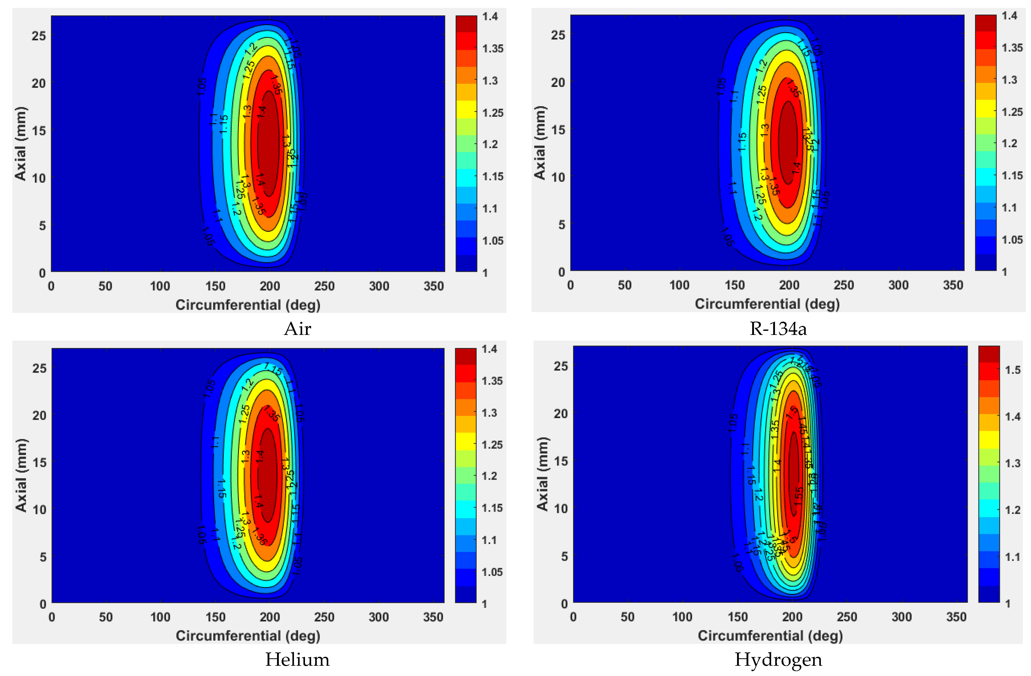
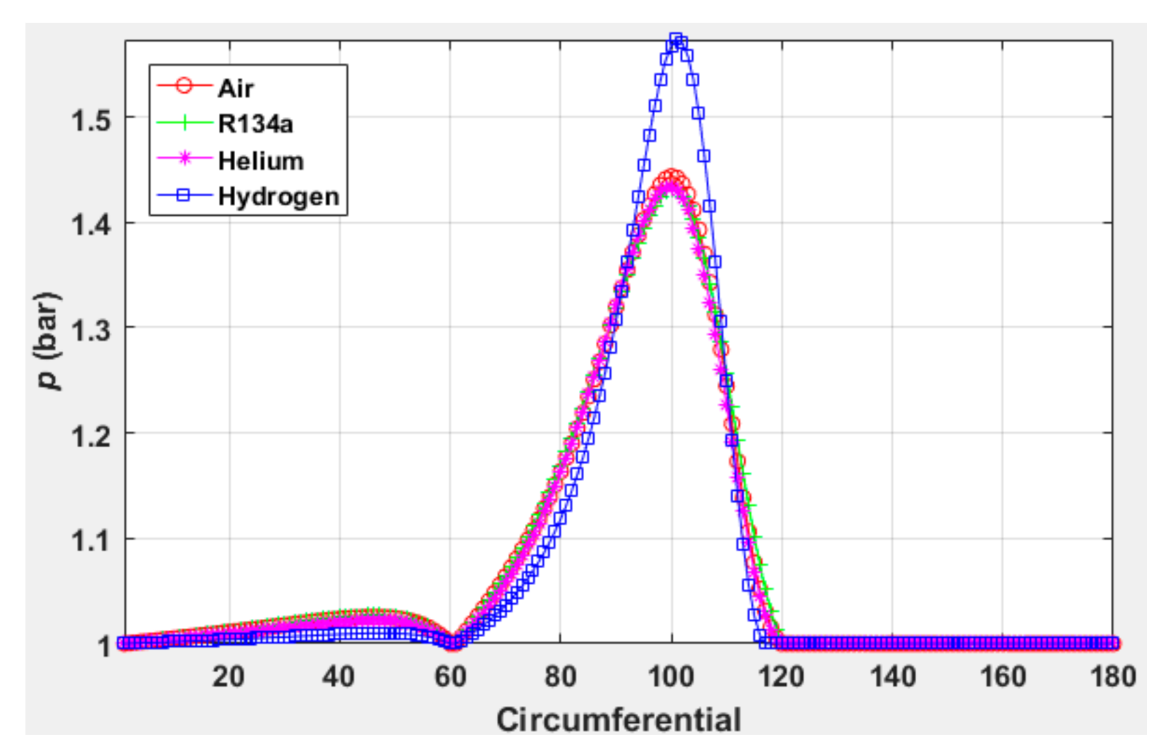
For the same operating conditions, we compare the static characteristics obtained for the following different gases: air, pentafluoropropane R-134a, helium R-704 and hydrogen R-702.
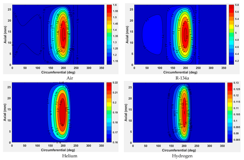
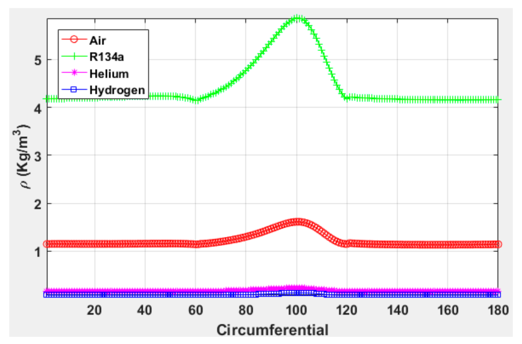
The pressure distribution shape (Figure 4 and Figure 5) is identical for the four gases, but we observe that the highest pressure is obtained for the hydrogen despite its lower initial viscosity. The “circumferential” coordinate shown in the various results is the global bearing coordinate, θb. The higher running density is obtained for R134a (Figure 6 and Figure 7). These results are consistent with the thermodynamic properties of these gases presented in Appendix B. The increase in the density at the mid-circumferential location is due to a high pressure existing in this zone. As air presents the highest magnitude of density against pressure, it is it is normal to get an upward shifted curve for air (Figure 7).
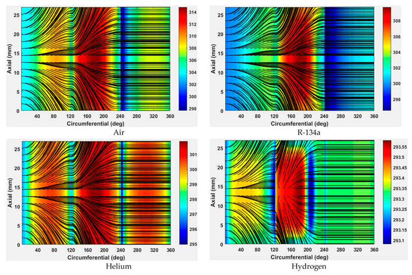
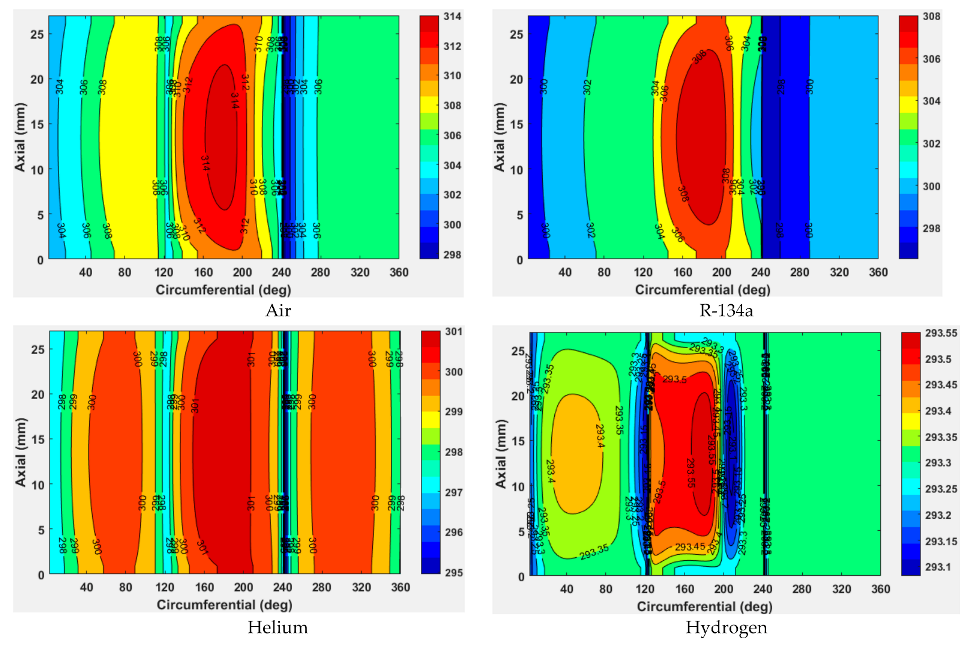
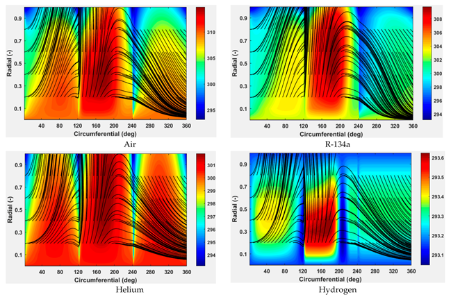
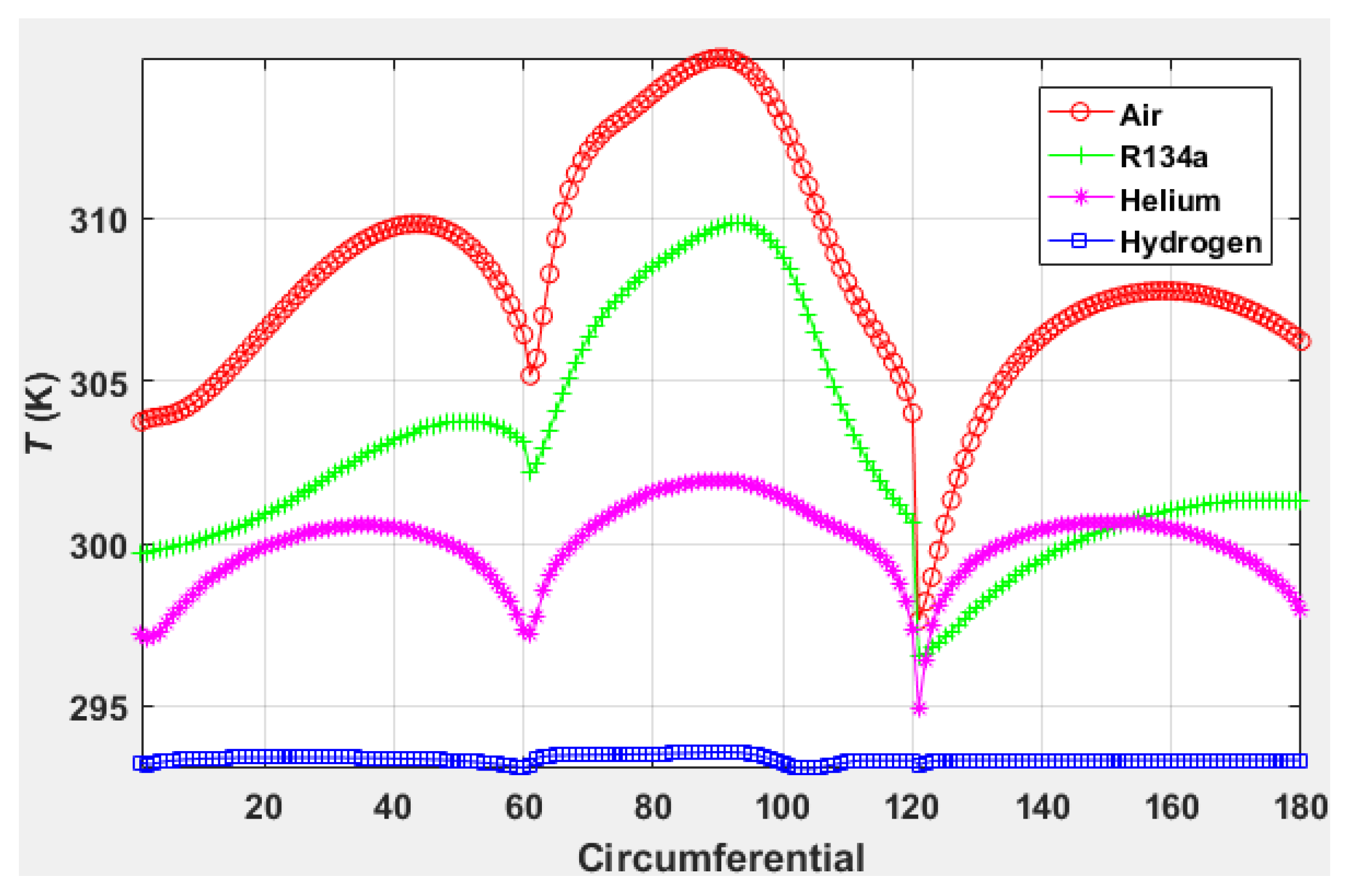
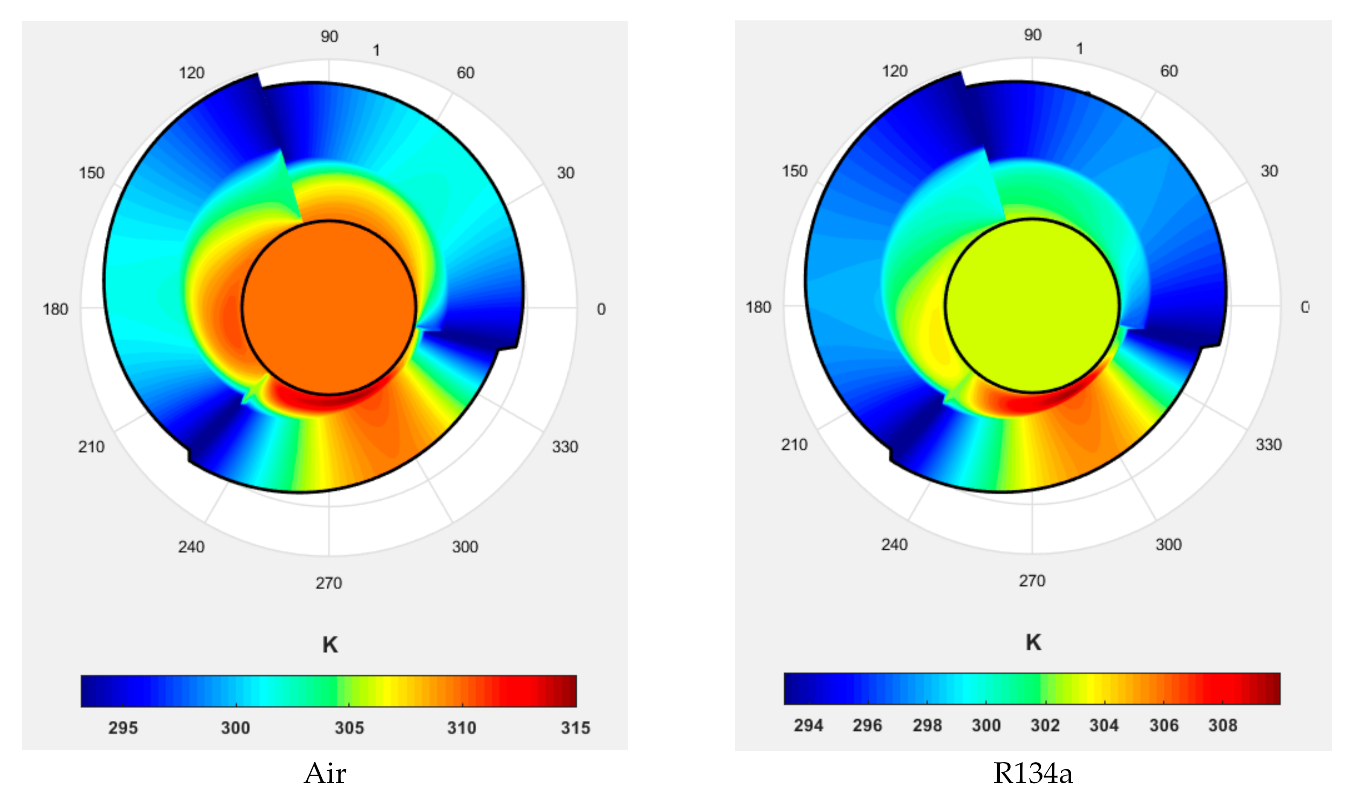
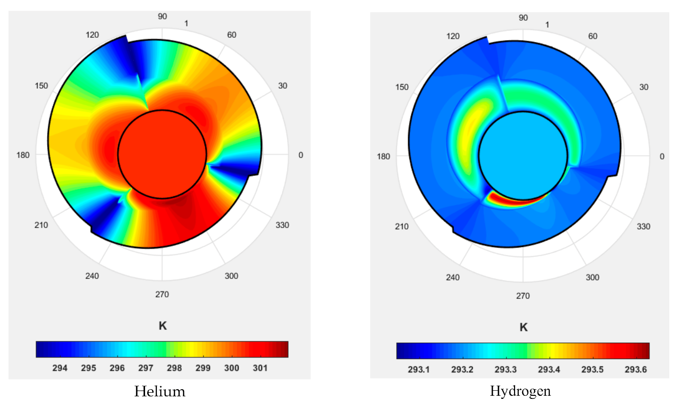
The temperature distributions are given in the following Figure 8, Figure 9, Figure 10, Figure 11, Figure 12 and Figure 13. We observe the same comparative aspects of temperature distribution as for density. If we refer to the curves given in Appendix B and more specifically the changes in density as a function of temperature, it is quite logical to observe the distribution profiles presented in Figure 11. Figure 8, Figure 10, Figure 11 and Figure 12, allow a better understanding of how the temperature is distributed in the film and in the housing. The operating conditions are the same for the four gases, and the orders of magnitude as well as the shapes of the distributions are quite similar.
Figure 12 below gives the temperature distribution in the solid materials (shaft and housing).
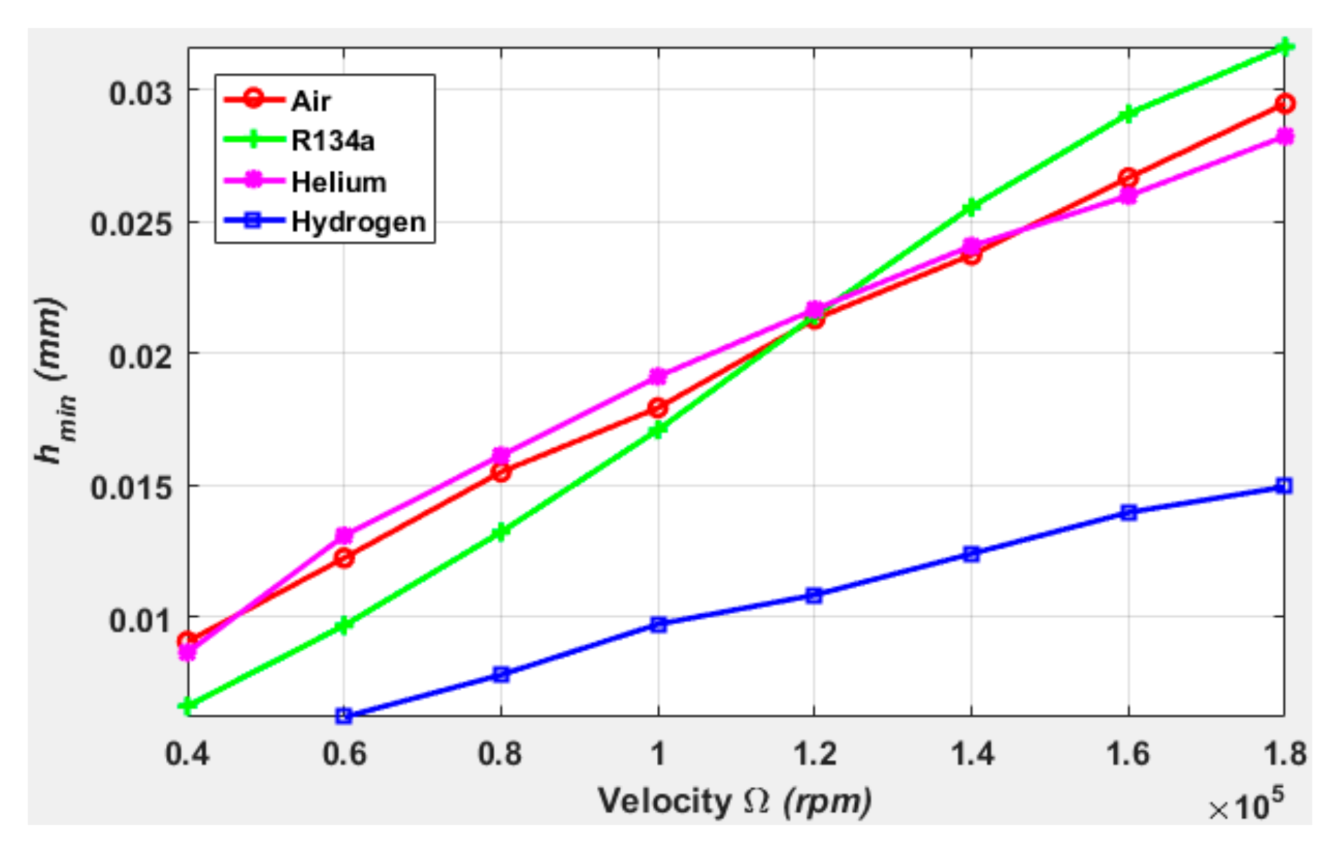
By virtue of its specific thermodynamic properties, hydrogen lubrication is less dissipative, and as its viscosity and density are low it gives a lower film thickness value than the others (see Figure 13).
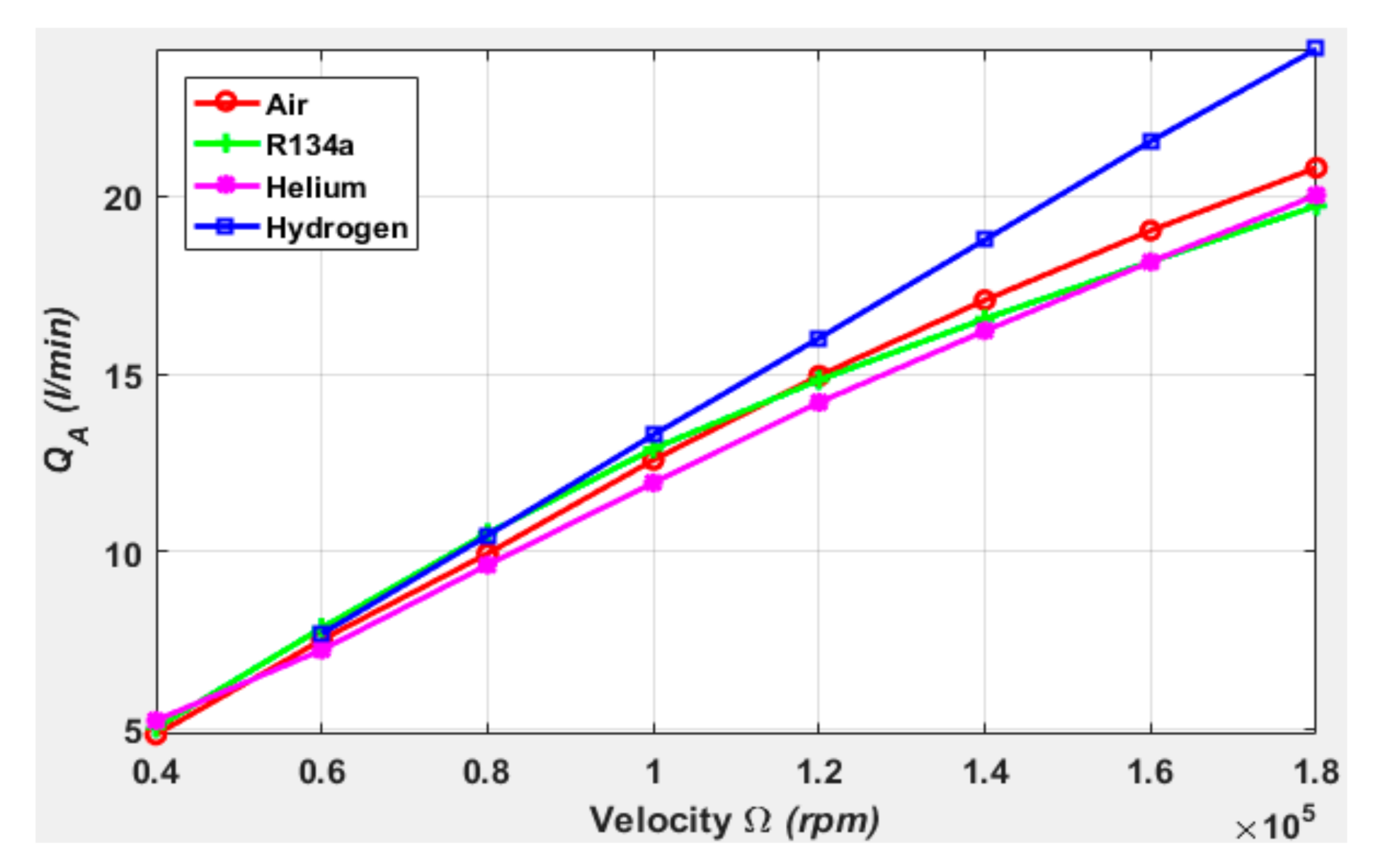
There are no strong differences in the variation of flow versus speed for velocities lower than 100,000 rpm, as shown in Figure 14. More hydrogen is needed to lubricate the contact as the speed increases.
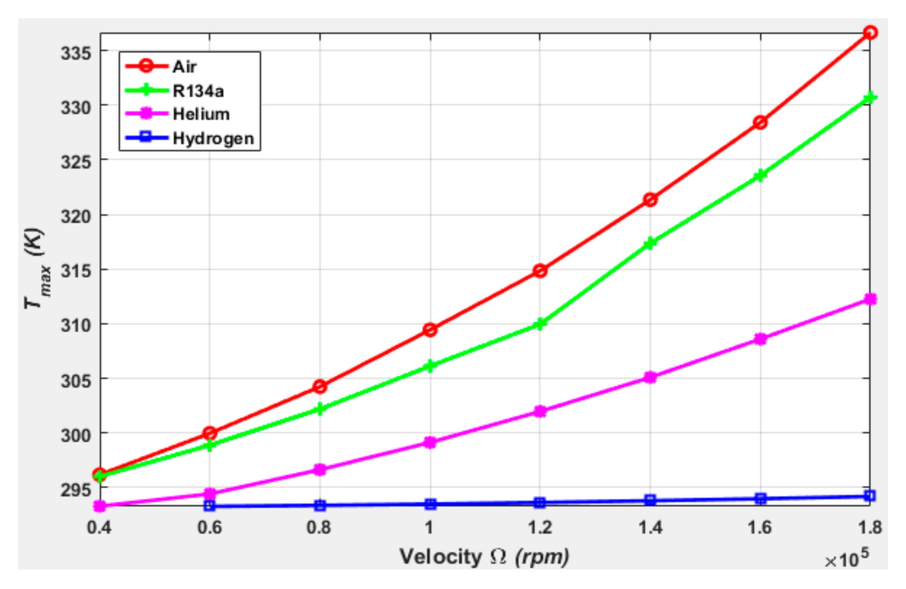
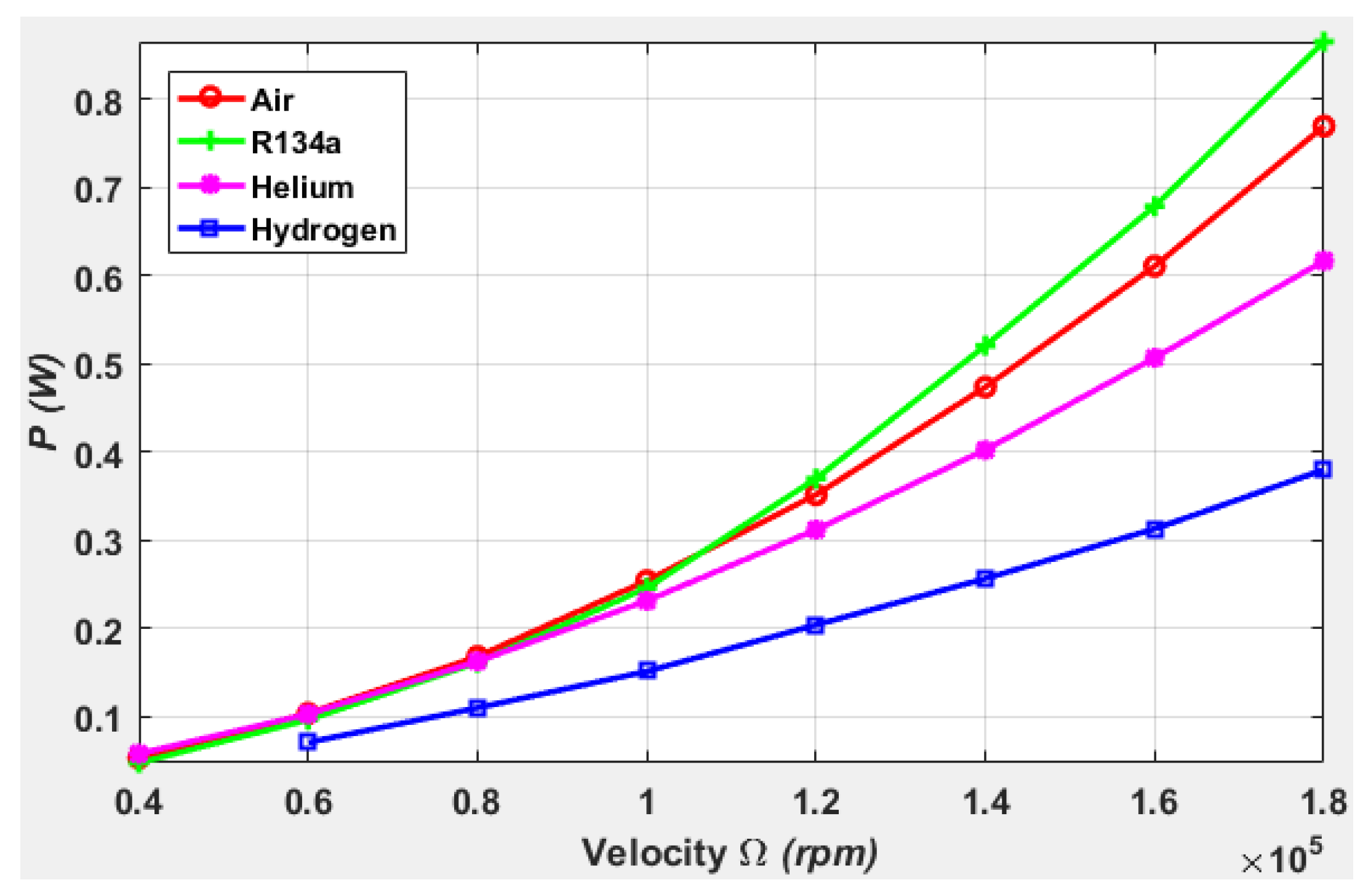
The changes in frictional torque as a function of the speed on the shaft and the housing are given in Figure 15. These results are consistent with those obtained for the maximum temperature evolution with speed, Figure 16, and power loss evolution in Figure 17. In calculations of local temperature, the effective viscosity (including the effect of turbulence) changes, but up to a factor of five. We do not show this result to conserve space on the already lengthy paper.
14. Conclusions
To extend the range of their application, we studied the behavior of different refrigerating gases, and other gases, in static and linear dynamic conditions of a lobed bearing. As these bearings are intended to run at very high rotation speeds, thermal and dynamic aspects must be considered. In this study, we showed the importance of an accurate description of the bearing, notably in these special lubrication conditions. Nonlinear phenomena are coupled, and the influence of temperature and thermodynamic gas properties have been primarily investigated. For the tested cases, we have found that the use of such gases as a lubricant is possible with a more complete study of their behavior, including the evolution of their thermodynamic properties in the contact.
Author Contributions
Conceptualization, B.B. and B.B.-S.; methodology B.B. and B.B.-S.; software, B.B.; validation, J.T.; formal analysis, B.B., B.B.-S. and J.T.; investigation, B.B., B.B.-S. and J.T.; resources, B.B., B.B.-S. and J.T.; data curation, B.B., B.B.-S. and J.T.; writing—original draft preparation, B.B.-S.; writing—review and editing, J.T.; visualization, B.B., B.B.-S. and J.T.; supervision, B.B.-S.; project administration, B.B.-S.; funding acquisition, B.B.-S. All authors have read and agreed to the published version of the manuscript.
Funding
Own fundings.
Institutional Review Board Statement
Not applicable.
Informed Consent Statement
Not applicable.
Data Availability Statement
Not applicable.
Conflicts of Interest
The authors declare no conflict of interest.
Nomenclature
| Cb | Bearing assembling clearance (m) |
| CL | Bearing manufacturing clearance (m) |
| Ci, i = 1,3 | Phenomenological constants in Clapeyron’s formula |
| cp | Heat capacity (J·kg−1·K−1) |
| Rs | Shaft radius (m) |
| Rh | Housing radius (m) |
| RL | Sector radius (m) |
| L | Bearing axial length (m) |
| F0 | Viscosity integral coefficient F0 (m2·s·kg−1) |
| F1 | Viscosity integral coefficient F1 (s) |
| F2 | Viscosity integral coefficient F2 (m·s) |
| h | Film thickness (m) |
| Nd | Dissipation number |
| psat | Vapor pressure (bar) |
| Pe | Peclet number |
| Local Reynolds number | |
| aρ | EoS temperature-dependent coefficient |
| cmin | Minimal speed of sound in the mixture (m:s−1) |
| cv | Minimal speed of sound in the vapor (m:s−1) |
| B | EoS constant coefficient (for a given fluid) |
| M | Molar mass (kg·mol−1) |
| k, k-, k- | Thermal conductivity (W·m−1·K−1) |
| h- | Global coefficient of exchange (W·m−2·K−1) |
| mρ | EoS constant coefficient (for a given fluid) |
| p | Pressure (Pa) |
| pc | Critical pressure (Pa) |
| Prt | Prandtl number |
| R | Ideal gas constant (J·mol−1·K−1) |
| T, T- | Temperature (K) |
| Tamb | Ambient temperature (K) |
| Tc | Critical temperature (K) |
| Tac | Critical Taylor number |
| TaL | Local Taylor number |
| u,v,w | Circumferential, radial and axial velocity components (m·s−1) |
| x,y,z | Circumferential, radial and axial coordinates (m) |
| y+ | Dimensionless distance from the wall |
| Su | Sutherland number |
| QE | Flow rate at the entry of sector (m3·s−1) |
| QS | Flow rate at the exit of sector (m3·s−1) |
| QA | Flow rate in the axial direction (m3·s−1) |
| W, W- | Load (N) |
| ki | Stiffness coefficient in the local coordinates (x,y,z) (N·m−1) |
| Ki | Stiffness coefficient in the global coordinates (r,t,z) (N·m−1) |
| ci | Damping coefficient in the local coordinates (x,y,z) (N·s·m−1) |
| Ci | Damping coefficient in the global coordinates (r,t,z) (N·s·m−1) |
| t | Time (s) |
| Mc | Critical mass (kg) |
| Keq | Equivalent stiffness (N·m−1) |
| Greek symbols. | |
| Λ | Bearing number |
| Ω | Shaft rotational speed (r.p.m) |
| ρ, ρ- | Fluid mass density (kg·m−3) |
| ϕe | Local attitude angle |
| ϕ | Global attitude angle |
| α | Volume expansivity at constant pressure (K−1) |
| αf | Heat transfer diffusivity |
| δL | Thickness of the laminar sublayer (m) |
| εi | Eccentricity ratio of sector |
| εb | Eccentricity ratio of bearing |
| θ, θb | Circumferential coordinate of a lobe, circumferential coordinate the bearing, see Figure 3 |
| κ | Von Karman constant |
| μ, μ-, μ- | Dynamic viscosity (Pa·s) |
| ωρ | EoS acentric factor |
| τ | Stress tensor (kg·m−1·s−2) |
| λ | Mixing coefficient |
| γc | Whirl frequency (Hz) |
| Subscripts, Superscripts. | |
| .* | Superscript for the sum of the laminar and turbulent parameter values |
| .t | Superscript for the turbulent regime |
| .0 | Subscript for the reference value |
| .l | Subscript for the liquid phase |
| .v | Subscript for the vapor phase |
| .s | Subscript for the shaft |
| .h | Subscript for the housing |
Appendix A. Bearing Geometry
The number of sector n.
The circumferential amplitude βi and axial length L of the sectors.
The amplitude of the circumferential groove γi.
Radius RL of sectors, Rs of the shaft and Rh of the housing.
The geometric pre-load a, which corresponds to the distance between the geometric center of the bearing and the center of curvature sector.
The position of the sectors an arbitrary fixed direction (O,X) (load direction) characterized by the angular coordinates θLi and ψLi, the angle θLi positions the beginning of the sector (i) to the load direction and ψLi marks its center line in a centered position.
Knowledge of these variables is used to define the following:
- -
- Radial assembly clearance: Cb = Rh − Rs;
- -
- Radial machining game: CL = RL − Rs;
- -
- The geometric precharge dimensionless coefficient m = 1 (Cb/CL);
- -
- The relative eccentricity εb = eb/Cb, with eb distance OOs.
The position of the shaft center is characterized by eccentricity (εb = eb/Cb) and attitude angle ϕ (Figure A1). Knowing these two parameters, we determine the relative position of each of the shaft sectors.
Figure A1.
Geometric details of bearing.

The dimensionless eccentricity ratio for each lobe dimensionless variable is as follows:
The angle ϕi, which characterizes the angle between the line of the centers of the sector (OiOs) with the line (OiO) is as follows:
with the following:
The symbol χi denotes the angle that characterizes the beginning of each sector, as follows:
for the calculation of the attitude angle, and angle δi between the load of sector Wi and load of bearing W (Figure A1) is as follows:
The load Wi and attitude angle ϕe for each sector in the coordinate system are determined by the following:
where the following applies:
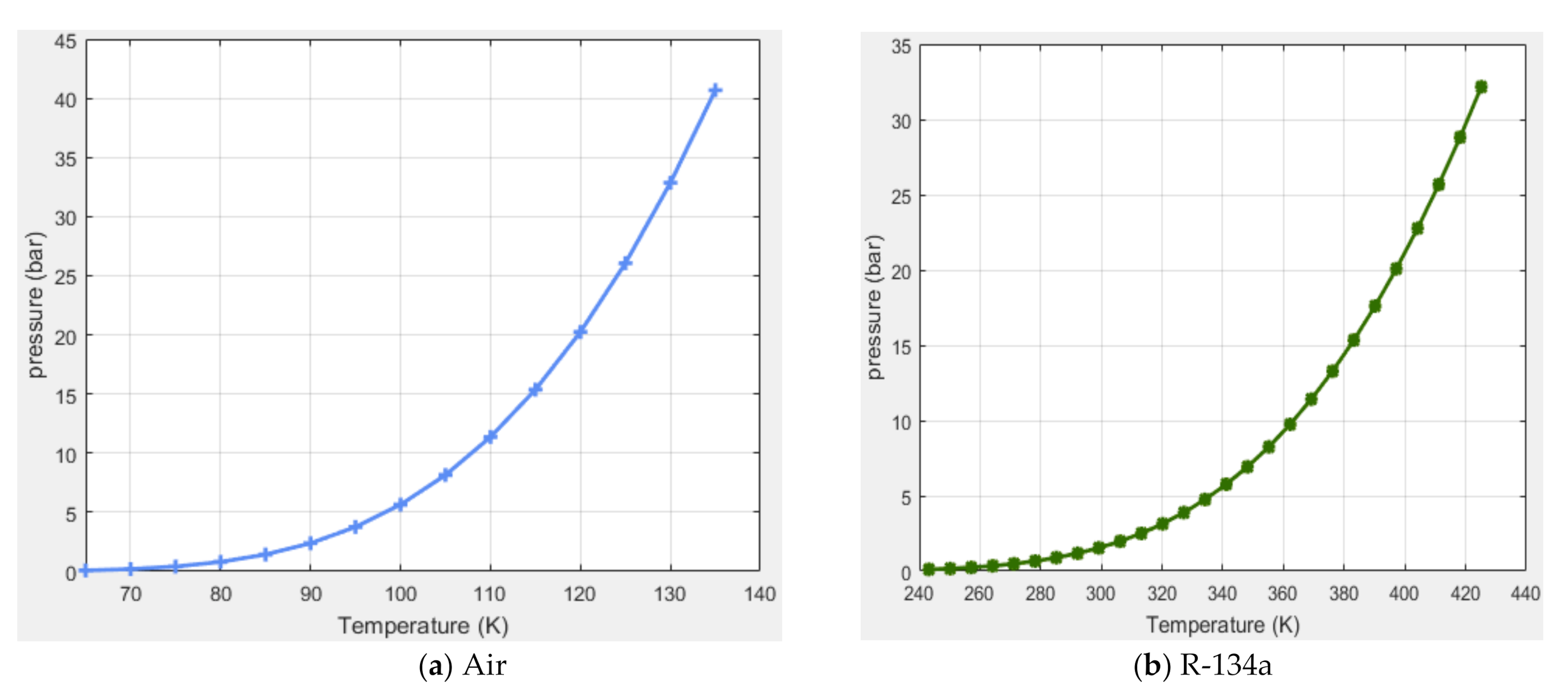
Appendix B. Lubricant Properties
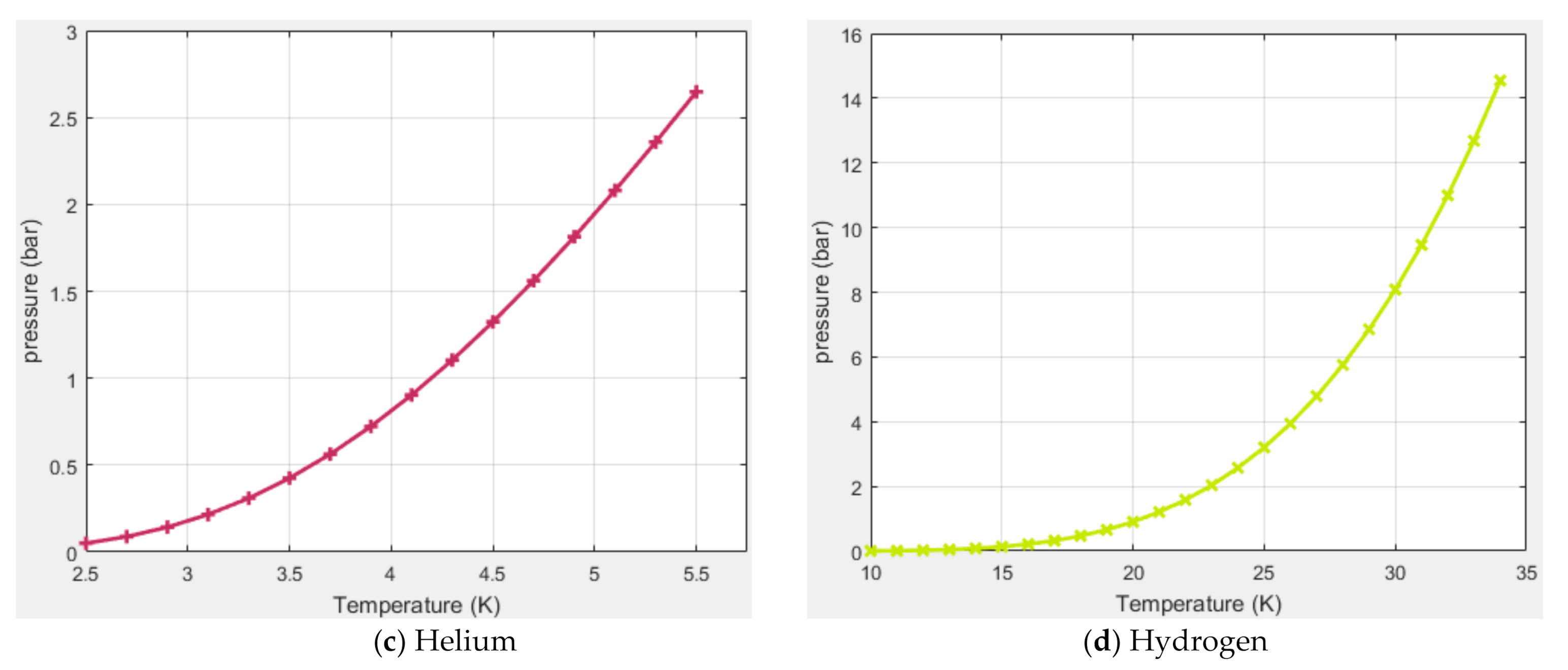
Figure A2.
Clapeyron diagram.


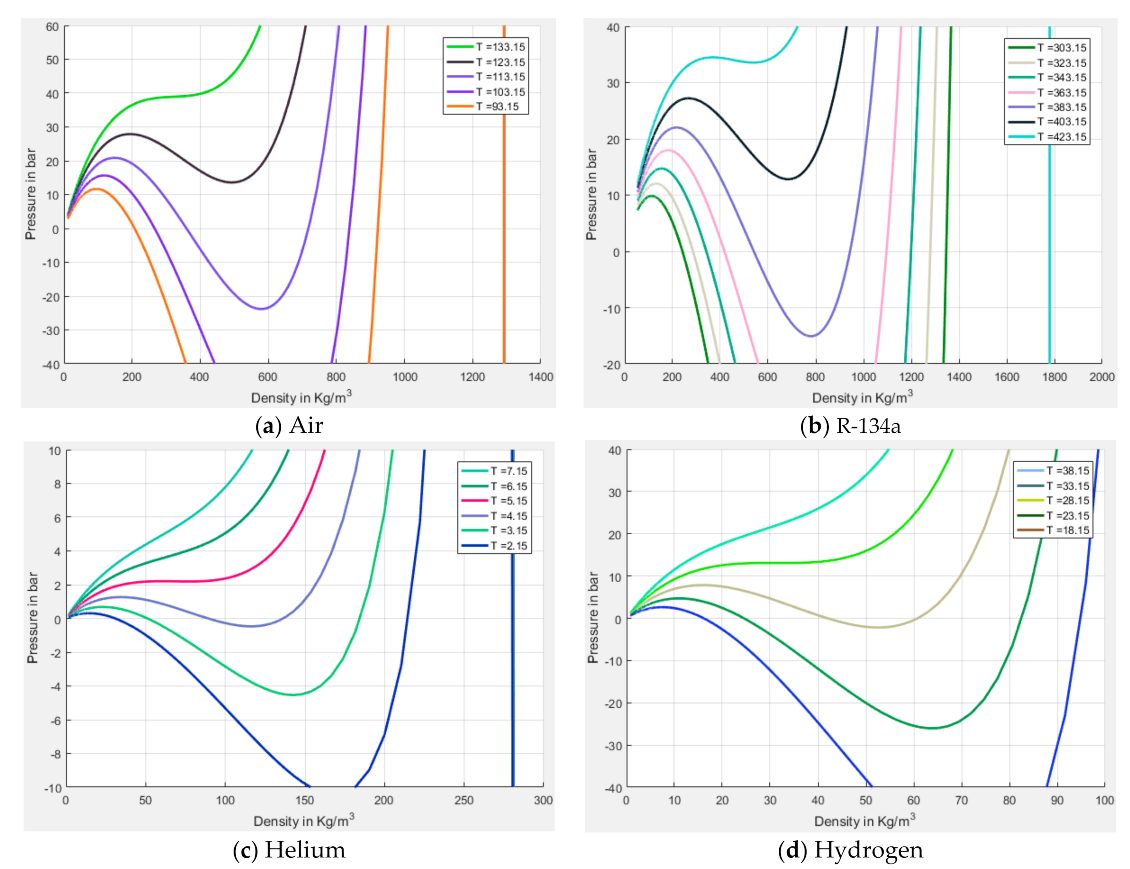
Figure A3.
Density versus pressure.

Appendix C
Figure A4.
Flow chart of the global numerical algorithm.

References
- Agrawal, G. Foil Air/Gas Bearing Technology an Overview. In International Gas Turbine & Aero-Engine Congress & Exhibition; ASME Paper: Orlando, FL, USA, 1997. [Google Scholar]
- Heshmat, H.; Walowit, J.; Pinkus, O. Analysis of gas-lubricated foil journal bearings. J. Lubr. Technol. 1983, 105, 647–655. [Google Scholar] [CrossRef]
- Xiong, L.; Wu, G.; Hou, Y.; Liu, L.; Ling, M.; Chen, C. Development of aerodynamic foil journal bearings for a high speed cryogenic turbo expander. Cryogenics 1997, 37, 221–230. [Google Scholar] [CrossRef]
- San Andres, L. Turbulent flow foil bearings for cryogenic applications. J. Tribol. 1995, 117, 185. [Google Scholar] [CrossRef]
- Nowak, P.; Kucharska, K.; Kaminski, M. Ecologiacal and Health Effects of Lubricant Oils Emitted into the Environment. Int. J. Environ. Res. Public Health 2019, 16, 3002. [Google Scholar] [CrossRef] [PubMed] [Green Version]
- Pei, H.; Li, F.; Chen, Y.; Huang, J.; Shen, C. Influence of biodegradable lubricant on the ecology, lubrication and achining process in minimum quality lubrication. Int. J. Adv. Manuf. Technol. 2021, 113, 1505–1516. [Google Scholar] [CrossRef]
- Dragicevic, M. The Application of Alternative Techniques for Cooling, Flushing and Lubrication to Improve Efficiency of Machining Processes. Teh. Vjesn. 2018, 25, 1561–1568. [Google Scholar]
- Nair, S.; Nair, K.; Rajendrakumar, P. Evaluation of physicochemical, thermal and tribological properties of sesame oil: A potential agricultural crop base stack for eco-friendly industrial lubricants. Int. J. Agric. Resour. Gov. Ecol. 2017, 13, 77–90. [Google Scholar] [CrossRef]
- Pereira, O.; Rodríguez, A.; Fernández-Abia, A.; Barreiro, J.; de Lacalle, L.L. Cryogenic and minimum quantity lubrication for an eco-efficiency turning of AISA 304. J. Clean. Prod. 2016, 139, 440–449. [Google Scholar] [CrossRef]
- Peng, D.; Robinson, D. A new two-constant equation of state. Ind. Eng. Chem. Fundam. 1976, 15, 59–64. [Google Scholar] [CrossRef]
- Lobo, L.; Ferreira, A. Phase equilibria from the exactly integrated Clapeyron equation. J. Chem. Thermodyn. 2001, 33, 1597–1617. [Google Scholar] [CrossRef] [Green Version]
- Odyck, D.; Venner, C. Compressible Stokes flow in thin films. J. Tribol. 2003, 125, 543–551. [Google Scholar] [CrossRef]
- Bohn, D. Environmental effects on the speed of sound. J. Audio Eng. Soc. 1988, 36, 223–231. [Google Scholar]
- Dowson, D. A generalized Reynolds equation for fluid-film lubrication. Int. J. Mech. Sci. 1962, 4, 159–170. [Google Scholar] [CrossRef]
- Garcia, M.; Bou-Saïd, B.; Rocchi, J.; Grau, G. Refrigerant Foil Bearing Behavior. A Thermo-HydroDynamic Study (Application to Rigid Bearings). Available online: http://0-dx-doi-org.brum.beds.ac.uk/10.1016/j.triboint.2012.12.006 (accessed on 3 June 2021).
- Frêne, J.; Nicolas, D.; Degueurce, B.; Berthe, D.; Godet, M. Lubrification Hydrodynamique: Paliers et Butées; Eyrolles: Paris, France, 1990. [Google Scholar]
- Reichardt, H. Vollstindige Darstellung der turbulenten Geschwindigkeitsverteilung in glatten Leitungen. ZAMM-J. Appl. Math. Mech. 1951, 31, 208–219. [Google Scholar] [CrossRef]
- Ng, C. Fluid dynamic foundation of turbulent lubrication theory. Asle Trans. 1964, 7, 311–321. [Google Scholar] [CrossRef]
- Hinze, J. Turbulence; Mcfirau Hill: New York, NY, USA, 1959. [Google Scholar]
- Dowson, D.; Hudson, J.D.; Hunter, B.; March, C.N. An experimental investigation of the thermal equilibrium of steadily loaded journal bearings. In Proceedings of the Institution of Mechanical Engineers; Sage: London, UK, 1966; Volume 181, Part 3B; pp. 70–80. [Google Scholar]
- Boncompain, R.; Fillon, M.; Frêne, J. Analysis of thermal effects in hydrodynamic journal bearings. ASME J. Tribol. 1986, 108, 219–224. [Google Scholar] [CrossRef]
- Boncompain, R. Les Paliers Lisses en Régime Thermohydrodynamique—Aspects Théoriques et Expérimen-Taux. Thèse de Doctorat d’état, Université de Poitiers, Poitiers, France, 1984. [Google Scholar]
- Xie, Z.; Zhang, Y.; Zhou, J.; Zhu, W. Theoretical and experimental research on the micro interface lubrication regime of water lubricated bearing. Mech. Syst. Signal Process. 2021, 151, 107422. [Google Scholar] [CrossRef]
- Bouyer, J.; Fillon, M. On the significance of thermal and deformation effects on a plain journal bearing subjected to severe operating conditions. J. Tribol. 2004, 126, 819. [Google Scholar] [CrossRef]
- Bruckner, R.; Dellacorte, C.; Prahl, J. Analytic Modeling of the Hydrodynamic, Thermal, and Structural Behavior of Foil Thrust Bearings; Report, NASA/TM2005-213811; NASA: Cleveland, OH, USA, 2005.
Figure 1.
Boundary conditions for temperature for a two-lobed bearing.

Figure 2.
Heat flux across the boundaries of the groove region.

Figure 3.
Schematic of the bearing. Left-hand side: an individual lobe, right-hand side: the global three-lobe configuration.
Figure 3.
Schematic of the bearing. Left-hand side: an individual lobe, right-hand side: the global three-lobe configuration.

Figure 4.
Contours of constant pressure, bearing load 10 N, shaft speed 120,000 rpm, preload m = 0.2.
Figure 4.
Contours of constant pressure, bearing load 10 N, shaft speed 120,000 rpm, preload m = 0.2.

Figure 5.
Pressure at axial mid-length, bearing load 10 N, shaft speed 120,000 rpm, preload m = 0.2.
Figure 5.
Pressure at axial mid-length, bearing load 10 N, shaft speed 120,000 rpm, preload m = 0.2.

Figure 6.
Contours of constant density 120,000 rpm, preload m = 0.2.

Figure 7.
Density at axial mid-length, bearing load 10 N, shaft speed 120,000 rpm, preload m = 0.2.

Figure 8.
Temperature field and streamlines at mid-film thickness (axial/circumferential), bearing load 10 N, shaft speed 120,000 rpm, preload m = 0.2.
Figure 8.
Temperature field and streamlines at mid-film thickness (axial/circumferential), bearing load 10 N, shaft speed 120,000 rpm, preload m = 0.2.

Figure 9.
Temperature at mid-film thickness (in the radial sense), bearing load 10 N, shaft speed 120,000 rpm, preload m = 0.2.
Figure 9.
Temperature at mid-film thickness (in the radial sense), bearing load 10 N, shaft speed 120,000 rpm, preload m = 0.2.

Figure 10.
Temperature field and streamlines at axial mid-length. Radial direction shown is fraction of the film thickness. Bearing load 10 N, Shaft speed 120,000 rpm, preload m = 0.2.
Figure 10.
Temperature field and streamlines at axial mid-length. Radial direction shown is fraction of the film thickness. Bearing load 10 N, Shaft speed 120,000 rpm, preload m = 0.2.

Figure 11.
Temperature distribution at axial mid-length, bearing load 10 N, shaft speed 120,000 rpm, m = 0.2.
Figure 11.
Temperature distribution at axial mid-length, bearing load 10 N, shaft speed 120,000 rpm, m = 0.2.

Figure 12.
Temperature distribution in the solids (shaft and housing).


Figure 13.
Film thickness versus shaft speed for the four gasses, bearing load 10 N, preload m = 0.2.
Figure 13.
Film thickness versus shaft speed for the four gasses, bearing load 10 N, preload m = 0.2.

Figure 14.
Flow rate versus shaft speed, bearing load 10 N, preload m = 0.2.

Figure 15.
Shaft frictional torque Ca and housing frictional torque Cc versus shaft speed, bearing load 10 N, preload m = 0.2.
Figure 15.
Shaft frictional torque Ca and housing frictional torque Cc versus shaft speed, bearing load 10 N, preload m = 0.2.

Figure 16.
Maximum film temperature versus shaft speed, bearing load 10 N, preload m = 0.2.

Figure 17.
Power loss versus shaft speed, bearing load 10 N, preload m = 0.2.

Figure 18.
Stiffness coefficients as functions of eccentricity ratio, shaft speed 100,000 rpm, preload m = 0.2.
Figure 18.
Stiffness coefficients as functions of eccentricity ratio, shaft speed 100,000 rpm, preload m = 0.2.

Figure 19.
Damping coefficients as functions of eccentricity ratio, shaft speed 100,000 rpm, preload m = 0.2.
Figure 19.
Damping coefficients as functions of eccentricity ratio, shaft speed 100,000 rpm, preload m = 0.2.


Table 1.
Bearing characteristics.
| Characteristics | Value |
|---|---|
| Length, | 27 |
| Shaft diameter, | 28 |
| Clearance, | 90 |
| Number of lobes | 3 |
| Eccentricity ratio, | 0.1–0.9 |
| Shaft speed, | 40,000–180,000 |
| Preload, | 0.2 |
| Amplitude of groove, | 10 |
| Global overall heat transfer coefficient, | 80 |
| Thermal conductivity, | 36 |
Table 2.
Fluid characteristics.
| Characteristics | Gas | |||
|---|---|---|---|---|
| AirR-729 | 1,1,1,3,3-Pentafluoropropane R-134a | Helium R-704 | Hydrogen R-702 | |
| Supply pressure | 1. | 1. | 1. | 1. |
| Supply temperature | 293.15 | 293.15 | 293.15 | 293.15 |
| Viscosity | 18.26 | 12.3 | 19.62 | 8.81 |
| Molar mass, | 28.95 | 134.05 | 4.0026 | 2.01594 |
| Heat capacity | 1006 | 976.9 | 5193 | 14290 |
| Thermal conductivity | 0.026 | 0.012 | 0.1535 | 0.18248 |
| Critical pressure | 37.878 | 36.51 | 2.2746 | 13.15 |
| Critical temperature | 132.53 | 427.16 | 5.2 | 33.19 |
| Acentric factor | 0.0335 | 0.32668 | −0.382 | −0.219 |
| Sutherland constants (-) | 120 | 110.4 | 79 | 72 |
Publisher’s Note: MDPI stays neutral with regard to jurisdictional claims in published maps and institutional affiliations. |
© 2021 by the authors. Licensee MDPI, Basel, Switzerland. This article is an open access article distributed under the terms and conditions of the Creative Commons Attribution (CC BY) license (https://creativecommons.org/licenses/by/4.0/).
Share and Cite
MDPI and ACS Style
Bouchehit, B.; Bou-Saïd, B.; Tichy, J. Towards Ecological Alternatives in Bearing Lubrication. Lubricants 2021, 9, 62. https://0-doi-org.brum.beds.ac.uk/10.3390/lubricants9060062
AMA Style
Bouchehit B, Bou-Saïd B, Tichy J. Towards Ecological Alternatives in Bearing Lubrication. Lubricants. 2021; 9(6):62. https://0-doi-org.brum.beds.ac.uk/10.3390/lubricants9060062
Chicago/Turabian StyleBouchehit, Bachir, Benyebka Bou-Saïd, and John Tichy. 2021. "Towards Ecological Alternatives in Bearing Lubrication" Lubricants 9, no. 6: 62. https://0-doi-org.brum.beds.ac.uk/10.3390/lubricants9060062
Note that from the first issue of 2016, this journal uses article numbers instead of page numbers. See further details here.