Digital Scanning of Welds and Influence of Sampling Resolution on the Predicted Fatigue Performance: Modelling, Experiment and Simulation

Abstract

Digital weld quality assurance systems are increasingly used to capture local geometrical variations that can be detrimental for the fatigue strength of welded components. In this study, a method is proposed to determine the required scanning sampling resolution for proper fatigue assessment. Based on FE analysis of laser-scanned welded joints, fatigue failure probabilities are computed using a Weakest-link fatigue model with experimentally determined parameters. By down-sampling of the scanning data in the FE simulations, it is shown that the uncertainty and error in the fatigue failure probability prediction increases with decreased sampling resolution. The required sampling resolution is thereafter determined by setting an allowable error in the predicted failure probability. A sampling resolution of 200 to 250 μm has been shown to be adequate for the fatigue-loaded welded joints investigated in the current study. The resolution requirements can be directly incorporated in production for continuous quality assurance of welded structures. The proposed probabilistic model used to derive the resolution requirement accurately captures the experimental fatigue strength distribution, with a correlation coefficient of 0.9 between model and experimental failure probabilities. This work therefore brings novelty by deriving sampling resolution requirements based on the influence of stochastic topographical variations on the fatigue strength distribution.

1. Introduction

A wide range of high-strength steel (HSS) engineering structures, such as loader cranes, transport vehicles and construction machinery, rely on welded joints for proper structural integrity. These joints are often the limiting factor for the fatigue strength of such load carrying structures. In order to assure durability and structural integrity in these applications, proper quality assurance methods of the welds are of the outmost importance.

Due to the stochastic nature of the welding process [1,2], local topographical variations in weld geometry are inevitable. This may result in local stress raising effects, such as sharp transitions and adverse undercuts. These quantities need to be quality assessed in production according to a weld quality system, to ensure the durability of the structure [3]. Traditionally, manual audits in which the actual weld geometry is measured, have been used for weld quality assurance. However, such manual systems, often hand-held simple tools, have shown to have limitations in accurately capturing local variations in the weld [4]. These limitations may be overcome by implementing digitalised weld quality assurance systems in production. This allows for a continuous quality control of welded joints with higher efficiency and accuracy than manual audits [4,5,6,7,8].

Given the scanned weld geometry obtained from the digitalized measurement system, the influence of local topographical variability can be assessed [9,10]. For this purpose, simulation approaches based on finite element (FE) analysis of the weld are predominantly used. Lang R. et al. [11,12,13], as well as Lener et al. [14], presented a framework for scanning and simulation of the weld geometry using a statistical approach and a Weakest-link fatigue model. It is noted that the influence of local surface defects is phenomenologically included in the Weakest-link model [15]. Niederwanger et al. [16] presented a comprehensive study where different fatigue modelling concepts were compared with regard to both idealised and measured weld geometry, captured using laser scanning. Kaffenberger and Vormwald [17,18] proposed modelling recommendations for idealized weld geometry simulations, based on the notch stress concept and 3D scanning of overlap and tee joints. Hou [19,20] and Chaudhuri et al. [21] modelled the measured 3D weld geometry to predict experimentally observed beachmark locations and crack measurements, respectively, based on weld toe stress concentration factors (SCF). Aldén et al. [22] performed detailed 3D simulations on cruciform joints of different weld classes showing that, while the maximum von Mises stress gives a good indication on the fatigue failure initiation location, it gives ambiguous predictions of the fatigue strength. Liinalampi et al. [23] investigated the fatigue strength of laser-hybrid welded fully penetrated butt joints based on 2D simulations of the measured weld geometry, captured using both stereo camera measurements as well as 3D laser microscopy. Ladinek et al. [24,25] studied the influence of measured weld geometry on fatigue life using a strain-life concept and Lang E. et al. [26,27] found that numerical simulations of the measured 3D geometry reproduce the experimental strain data for butt joints in the low cycle fatigue regime.

Although the aforementioned studies include the measured geometry of welded joints in detailed FE simulations, they lack the ability to identify the level of detail that is required for a proper fatigue assessment. In the current study, the sampling resolution is investigated for digitalized weld quality assurance systems which is required to accurately predict the fatigue performance. Based on the scanned topographies, a probabilistic weakest-link approach [28,29,30] is proposed. This work therefore provides the following scientific contribution.

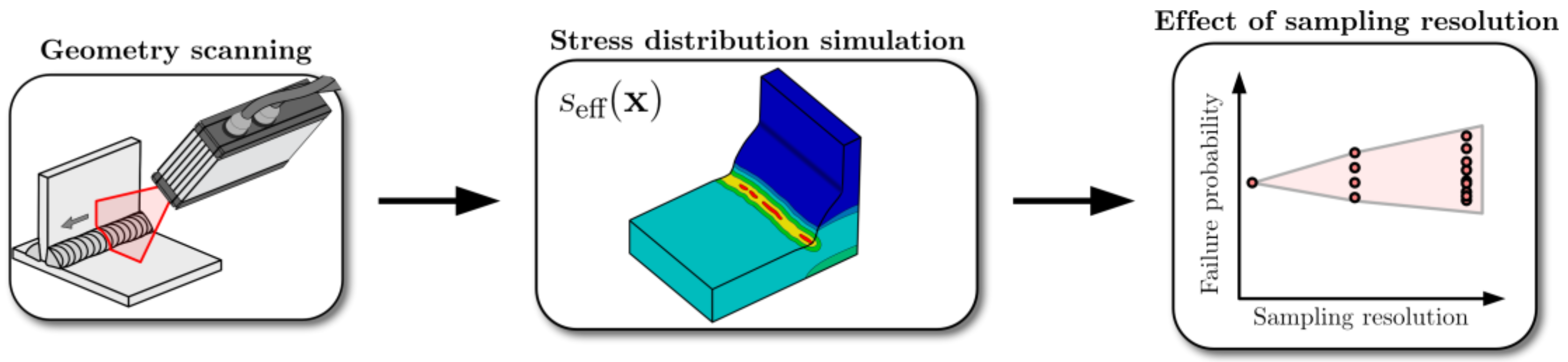
• A framework for determining the scanning resolution needed for digital quality assurance of welded joints that is assessed on non-load carrying tee joints. The resolution requirements can then be directly incorporated in production for continuous quality assurance of welded structures.
• A modelling approach to predict the fatigue strength probability distribution based on measured weld geometry variation.

An overview of the workflow is presented in Figure 1. Laser scanning of welded tee joints is first performed to accurately capture the measured weld topography, which is then evaluated using both an industrially commercial quality assurance system and detailed FE analysis. Based on the FE analysis of the scanned weld geometry, the fatigue failure probability is computed using a Weakest-link area model. The parameters in the model are determined by minimizing the error between experimental and simulated failure probabilities. Finally, the sensitivity of the computed failure probability for different sampling resolutions is determined based on FE simulations with different levels of topographical details.

2. Experimental Investigation

Single pass, non-load carrying, tee joint test specimens produced out of S700 steel were used as the basis for the probabilistic fatigue investigation in the present study. The geometry of the specimen is presented in Figure 2, together with the desired weld throat thickness and weld penetration. Post-treatment using High Frequency Mechanical Impact (HFMI) [31] was carried out on one side of the tee joint specimens to create an uneven distribution in the fatigue strength between the two welded sides. Only the un-treated weld will be further considered as the fatigue strength of this weld will be detrimental for the fatigue strength of the complete specimen.

The specimens were produced using a gas metal arc welding (GMAW) process in the PA position using a pushing travelling angle and a heat input of 0.62 kJ/mm. Sandblasting was used after the welding to remove slag and oxides, as this step helps ensure that the geometry captured in the scanning procedure is the actual geometry of the weld and not the oxide layer.

2.1. Topographic Scanning

The complete geometry of the un-treated weld seams is captured using a scanCONTROL 2950-50-line laser (Micro-Epsilon, Ortenburg, Germany). This unit has a pixel density of 1280 px/profile and the nominal length of the laser line that is 50 mm. The laser is operated using a robot arm which moves the projected laser line along the surface of the welded joint at a constant velocity while the laser unit continuously captures linear, 2D profiles at fixed intervals. This gives a point cloud database for each specimen containing the complete geometry of the scanned profiles with location data for each data point captured by the sensor matrix. The position of the measured points in each profile is given with reference to the measurement unit.

There are two resolutions that need to be considered when scanning welded joints—the reference profile resolution and the sampling resolution. The reference profile resolution is determined in the direction of the laser line by the pixel density of the sensor matrix and the nominal measurement length of the laser line. For this specific laser, the reference profile resolution is 39 μm. The sampling resolution is given as the distance between two sample profiles and is calculated using the scanning velocity and the scanning frequency, as presented in Figure 3. The highest resolution investigated in this study is 50 μm, which is also the resolution used when fitting the model parameters.

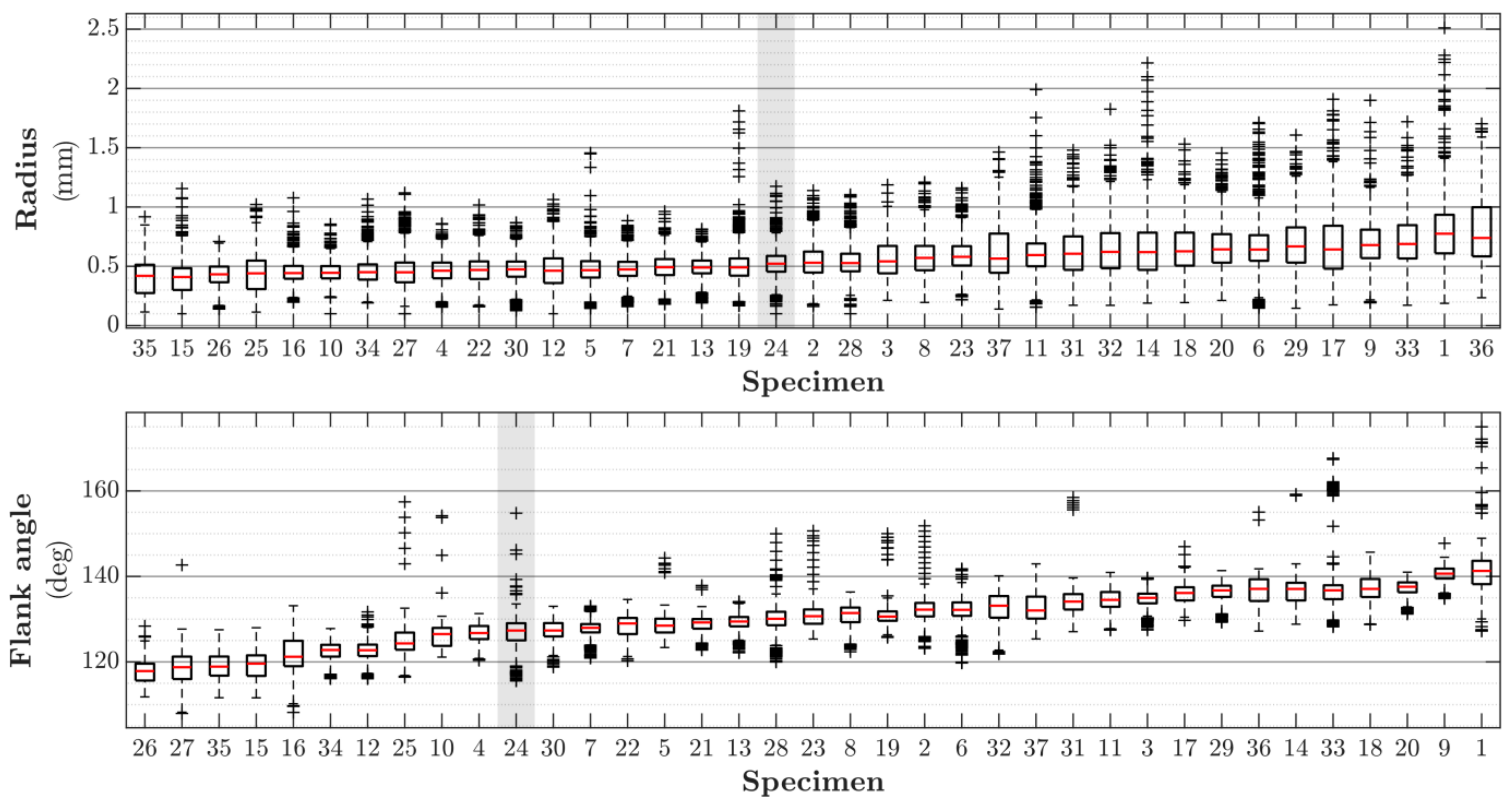
2.2. Weld Geometry Evaluation

The captured weld geometry is analysed using the commercial quality assurance system Winteria ^® qWeld (Winteria, Hudiksvall, Sweden) [32]. This is done to investigate and present the scatter in weld geometry for the investigated group of specimens independently from the simulations that is later carried out. This quality assurance system quantifies the weld geometry into geometric definitions as throat thickness, weld leg length, undercut, weld toe radius and weld toe angle using internal algorithms developed by Stenberg et al. [5,6]. The algorithm goes through each weld section with an internal algorithm which locates the weld toes and determines the weld toe radii and angle by a fitting routine. The accuracy of the method has been proven to be comparable to other commercial programs when the same reference block has been studied [5]. The accuracy has also been studied in [6]. The latter two geometrical parameters are presented in Figure 4 along the weld surface of specimen 24.

The variation in radius and weld toe angle between the tested specimens is presented in Figure 5. The scatter of the mean weld toe radius between the specimens is less than 0.5 mm and the corresponding scatter for the weld toe angle is approximately 20 degrees. The mean value of the weld toe radius for the investigated specimens is 0.56 mm with a standard deviation of 0.21 mm for the group. There are some specimens where outliers with smaller radii are visible, which potentially indicates the presence of local regions where high stress concentrations can be expected. One of these is the previously mentioned specimen 24 where a sharp corner can be seen at the 50 mm position. This specimen is of interest as its mean values for both presented parameters are representative for the group of specimens, while it has a large number of outliers below the mean for both parameters.

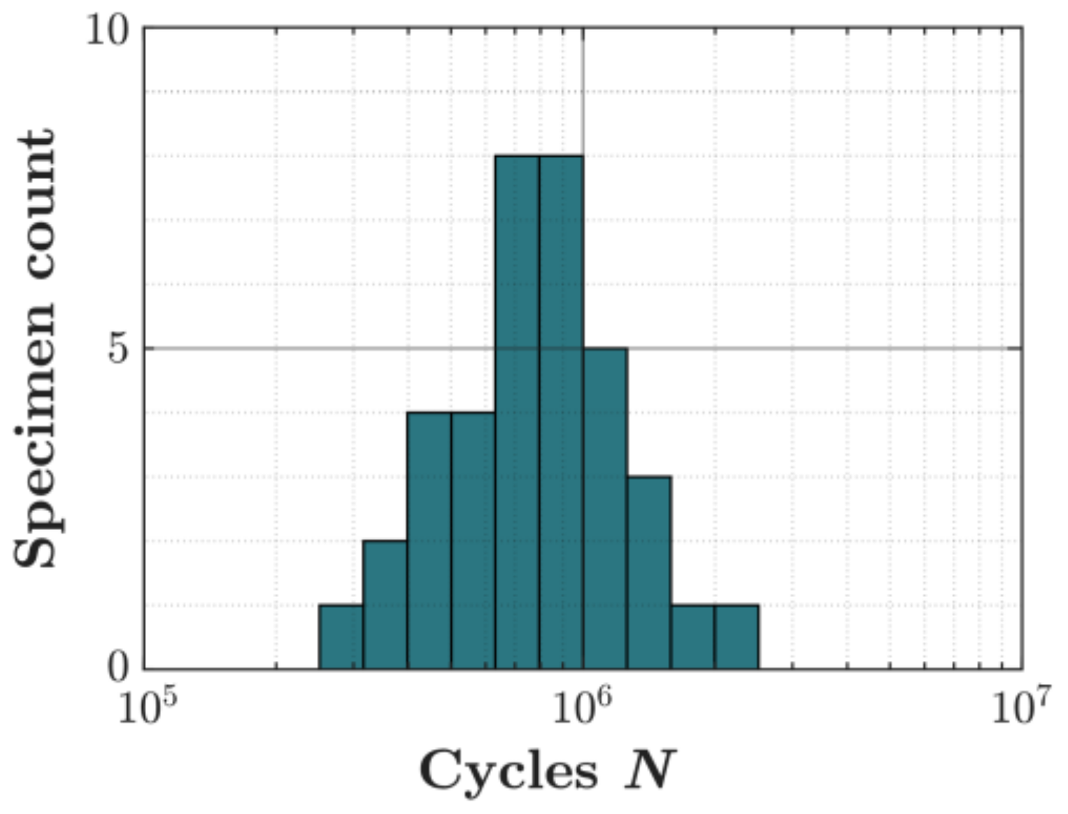
2.3. Uniaxial Fatigue Testing

Constant amplitude fatigue testing was carried out using an MTS High-Force Servo hydraulic tensile tester (MTS, Eden Prairie, MN, USA) at a load ratio of 0.1. All specimens were tested at a load level of 180 MPa. A total of 51 specimens were tested, and 14 of those were stopped at 5 million cycles as no failure had occurred. The test results for the failed specimens are presented both in Figure 6 and

Table 1. Fatigue test data for single-pass tee joint test specimens and median rank estimates. All specimens are fatigue-loaded at R = 0.1 and amplitude 180 MPa.

Failure Order i	Cycles [-]	Median Rank, ${\mathit{p}}_{\mathbf{f},\mathit{i}}^{\mathbf{exp}}$	Failure Order i	Cycles	Median Rank, ${\mathit{p}}_{\mathbf{f},\mathit{i}}^{\mathbf{exp}}$
1	296319	0.0187	20	796070	0.5267
2	319754	0.0455	21	844067	0.5535
3	358569	0.0722	22	874843	0.5802
4	450880	0.0989	23	875982	0.6070
5	479592	0.1257	24	911631	0.6337
6	491902	0.1524	25	942420	0.6604
7	499422	0.1791	26	978798	0.6872
8	554425	0.2059	27	998173	0.7139
9	577447	0.2326	28	1017389	0.7406
10	601596	0.2594	29	1067794	0.7674
11	621224	0.2861	30	1102915	0.7941
12	637281	0.3128	31	1159417	0.8209
13	644313	0.3396	32	1199808	0.8476
14	697257	0.3663	33	1259817	0.8743
15	707011	0.3930	34	1478800	0.9010
16	712686	0.4198	35	1563887	0.9278
17	739705	0.4465	36	1960249	0.9545
18	761384	0.4733	37	2418827	0.9813
19	781303	0.5

. Only the specimens that failed are processed further in this study.

The experimental failure probability was determined for the 37 specimens that failed using an approximation for median ranks proposed by A. Benard [33],

$$p_{\mathrm{f},i}^{\exp } \approx \frac{i - 0.3}{n_{\mathrm{spec}} + 0.4}$$

(1)

This gives an approximative failure probability for the i:th ranked failure out of a population of $n_{\mathrm{spec}} = 37$ specimens at a 50% confidence level. The cumulative distribution function for the given group of specimens using Benard’s approximation is presented in Figure 7.

3. Probabilistic Fatigue Model

In the following, the probability distribution for the fatigue strength is derived based on the Weakest-link model [28,29].

3.1. Weakest-Link Area Model

The Weakest-link area model is derived from the assumption that fatigue failure is caused by cracks initiated at critical surface defects and that the distance between the defects is large enough not to cause any interaction between them. Assume that the number of such defects on a reference surface area $A_{\mathrm{ref}}$ is $q$. Assume further that the area $A_{\mathrm{ref}}$ is divided into $k$ small sub-areas and that all sub-areas are subjected to the same stress amplitude $S$. The probability to find a critical defect in the sub-area is then $q/k$. The probability of not finding a critical defect in a total number of $k$ sub-areas is therefore ${(1-q/k)}^k$. The probability of failure, i.e., the probability of finding a critical defect in $A_{\mathrm{ref}}$, can therefore be written as

$$p_{\mathrm{f}}^{\mathrm{WL}} = 1 - \underset{k\to \infty }{\lim }{\left(1 - \frac{q}{k}\right)}^k = 1 - \exp \left(-q\right).$$

(2)

The number of critical defects is assumed to increase with increased stress level $s$. A function proposed by Weibull that shows good agreement with experimental data is $q={(s/\lambda )}^{\beta }$ which results in

$$p_{\mathrm{f}}^{\mathrm{WL}} = F_S\left(s\right) = 1 - \exp \left[-{\left(\frac{s}{\lambda }\right)}^{\beta }\right],$$

(3)

where $F_S\left(s\right)$ is the Weibull probability distribution of the fatigue strength with scale and shape parameters $\lambda$ and $\beta$, respectively. It is noted that Equation (3) gives the fatigue failure probability for a uniaxial stress amplitude $S$ at a given number of cycles to failure $n$. The dependence on the number of cycles is given by the scale parameter $\lambda \left(n\right)$. An analytical expression of the form

$$\lambda \left(n\right) = {\lambda }_0{\left(\frac{n_0}{n}\right)}^{\frac{1}{m}}\exp \left[\frac{c_{\mathrm{EM}}}{\beta }\right]$$

(4)

has been proposed by the authors [30], where $m$ is the inverse Basquin exponent, $c_{\mathrm{EM}} \approx 0.5772$ is the Euler–Mascheroni constant, $n_0 = 2\times {10}^6$ is a reference number of cycles to failure and ${\lambda }_0$ is a fitting parameter. A value of $m = 3$ is recommended for as-welded components with normal weld quality [34]. Using Equation (4), it is noted that the expression for the failure probability according to Equation (3) has two unknown parameters, ${\lambda }_0$ and $\beta$, which will be determined in Section 5.

3.2. Multiaxial Considerations

The expression in Equation (3) can be generalized to be applicable for non-uniform stress distributions and multiaxial stress states acting on an area of arbitrary size. Assume that the measured weld area $A$, see Figure 8a, is subjected to a multiaxial stress distribution. Assume further that $s_{\mathrm{eff}}\left(x\right)$ is an effective local stress amplitude, where $x$ is a location vector. The probability of failure according to Equation (3) can be written as

$$p_{\mathrm{f}}^{\mathrm{WL}} = 1 - \exp \left[-{\left(\frac{s_{\mathrm{equ}}}{\lambda }\right)}^{\beta }\right],$$

(5)

where an equivalent stress amplitude is introduced according to

$$s_{\mathrm{equ}} = {\left[\frac{1}{A_{\mathrm{ref}}}{{\displaystyle \int }}_A{s}_{\mathrm{eff}}{\left(\mathit{x}\right)}^{\beta }dA\right]}^{\frac{1}{\beta }}.$$

(6)

It is noted that the integration is performed over the surface area $A$. From Equations (5) and (6) it is seen that if $A = A_{\mathrm{ref}}$ and $s_{\mathrm{eff}}\left(x\right) = s$, then $s_{\mathrm{equ}} = s$ and Equation (3) is recovered. It should be emphasized that Equation (5) is a conditional probability given a deterministic applied load [35] and a known measured topography of the weld area. Including random uncertainties in load and stress field is possible using methods from structural reliability [36,37,38,39,40] but is out of the scope of the present work.

The reference area, $A_{\mathrm{ref}}$, is taken as the local area of the idealised weld surface. This is idealised as the throat area of the weld bead with two extension regions at both weld toes with lengths ${\mathrm{l}}_{\mathrm{ext},\mathrm{x}}$ and ${\mathrm{l}}_{\mathrm{ext},\mathrm{y}}$, as seen in Figure 8 and

Table 2. Reference area parameters.

Parameter	Implemented Value
$\mathrm{a}$	4 mm
$\mathrm{w}$	60 mm
${\mathrm{l}}_{\mathrm{ext},\mathrm{x}}$	10 mm
${\mathrm{l}}_{\mathrm{ext},\mathrm{y}}$	8 mm
$\mathrm{t}$	6 mm
$A_{\mathrm{ref}}$	881.2 mm2

. It is possible to use either the measured mean value of the throat thickness for the group of specimens or the desired throat thickness, as the fitting procedure will account for any deviation between the two. The latter one is used in the present study. The distances of the extension regions are chosen so that all stress-raising effects near the weld toes are included in $A_{\mathrm{ref}}$. The idealised weld surface is not influenced by the measured geometry of individual specimens. The reference area must be large enough to accurately capture the stress distribution in the weld and the highly stressed region near the load-carrying weld toe for all investigated specimens. This needs to be fulfilled even for the most extreme variations in the local weld geometry seen in the group of specimens. The reference area is also chosen so it is smaller than the total area measured by the laser scanner, as this ensures that no extrapolation in the dataset is needed. The reference area is calculated as

$$A_{\mathrm{ref}} = \mathrm{w}\left[\left(1 - \sqrt{2}\right)2\mathrm{a} + {\mathrm{l}}_{\mathrm{ext},\mathrm{x}} + {\mathrm{l}}_{\mathrm{ext},\mathrm{y}}\right].$$

(7)

A common choice of effective stress is based on the largest principal stress ${\sigma }_1\left(x,t\right)$ which varies with time $t$. During the complete load cycle, the principal stress attains a maximum ${\sigma }_1^{\max }\left(x\right)$ and a minimum ${\sigma }_1^{\min }\left(x\right)$. The effective stress can be evaluated as [41]

$$s_{\mathrm{eff}}\left(x\right) = \frac{1}{2}\left[\max \left(0,{\sigma }_1^{\max }\left(x\right)\right) - \min \left(0,{\sigma }_1^{\min }\left(x\right)\right)\right],$$

(8)

which is applicable when the direction of ${\sigma }_1\left(x,t\right)$ is little affected by $t$. It is noted that a pulsating stress will be more decisive for the fatigue life than an alternating stress and that a point with only compressive stresses throughout the complete load cycle will not contribute to the failure probability.

It should be emphasized that the influence of surface defects is phenomenologically included in the Weakest-link model. Consider a hypothetical case where the surface topography is perfectly smooth without any variability, which corresponds to constant local stresses along the surface. The Weakest-link (WL) model according to Equation (5) still predicts a variability in the fatigue strength. The origin of this variability stems from the assumption that fatigue failure is caused by cracks initiated at randomly distributed critical surface defects that do not interact with each other. The size of this variability in fatigue strength is determined by the Weibull parameters, which are directly affected by surface defects, such as micropores and inclusions.

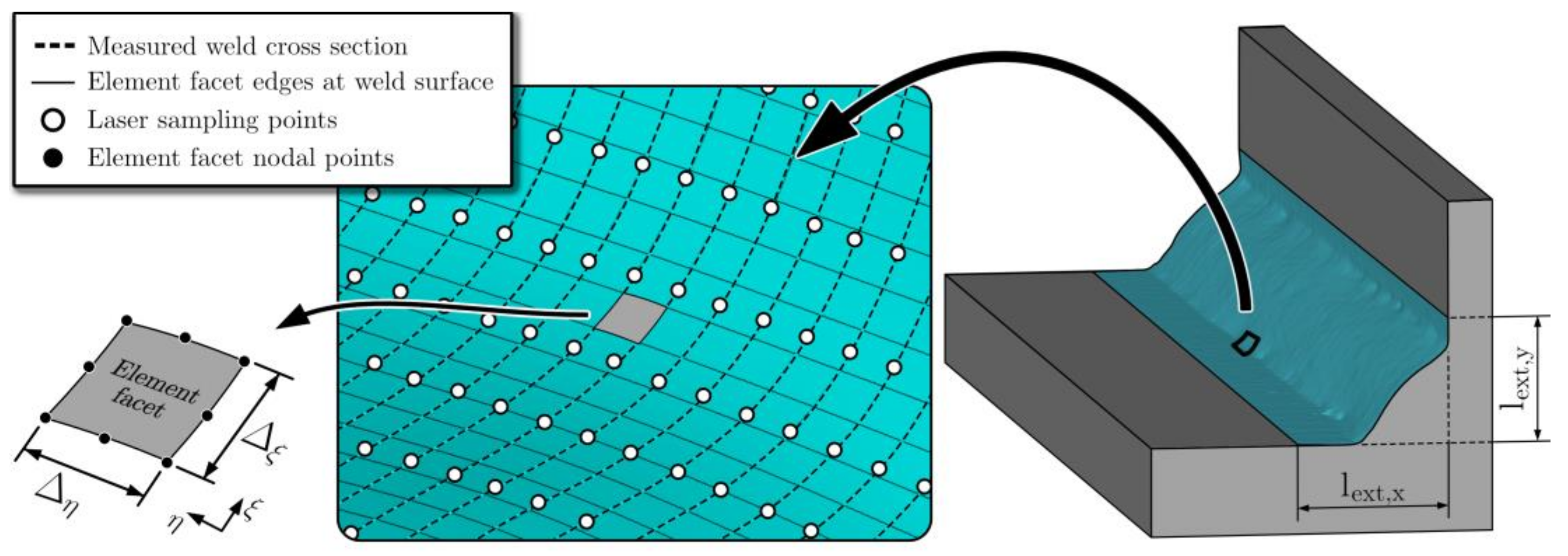
4. Numerical Implementation of True Weld Geometry

The detailed sectional geometry measurements were stitched together in a pre-processing algorithm to form the complete weld surface. Any unwanted skewness in the surface resulting from misalignments in the trajectory of the laser unit when scanning is corrected by affine transformations based on the relative angles of the plate and the transverse stiffener. Erroneous or missing data points are replaced with linearly interpolated points, no extrapolation is carried out as the final size of the reconstructed surface is truncated at the ends. Short wavelength noise in the recreated data set is removed using a Gaussian filter with a sampled Gaussian kernel. This is essential, as the un-filtered surface includes discontinuations not seen in the true weld surface, which can reduce the accuracy.

The pre-processed surface is then sent as database sampling points to ANSYS (2020 R2, ANSYS Inc, Canonsburg, PA, USA) where the local model of the welded joint is created, one weld profile at a time, using non-uniform rational basis spline (NURBS) surfaces. Once the complete local weld is created, it is merged with the nominal geometry to produce the complete specimen.

The solid model is discretised using tetrahedral and hexahedral brick elements with quadratic shape functions (SOLID 186 in Ansys). A structured mesh is prescribed on the weld surface so that the corner nodes of each element at the surface coincides with the measured weld cross-section profiles, as seen in Figure 9. The number of element facets that are tangential to the weld surface between two weld section profiles will therefore be the same throughout the topographic surface. The side length ${\Delta }_{\xi }$ of the element surface facets in the ξ direction does thus vary to a small extent. The mean value of ${\Delta }_{\xi }$ in the region close to the fatigue loaded weld toe is prescribed as 15 μm, whereas the remaining element surface facets have a mean value of 150 μm. The side length ${\Delta }_{\eta }$ of the element surface facets in the η direction is set to 50 μm.

Half of the specimen, including the non-treated weld, is modelled as a representative unit of fatigue strength for the complete specimen. This is motivated by the fact that no fatigue failure was initiated at the HFMI-treated weld. A symmetry boundary condition is applied on the symmetry plane going through the middle of the stiffener. The nodes located at the far end of the specimen, where the fatigue clamps grip, are slave nodes connected rigidly to remote master nodes that lie in corresponding z-planes, as schematically presented in Figure 10. These nodes are constraints from translation in all directions except for in the x-direction and they are only free to rotate around z.

Each specimen is simulated in two analysis steps—the first step represents the straightening of the specimen in the clamping phase (prescribed rotation θ = π − θ_p) and the second corresponds to the cyclic loading of the specimen (prescribed rotation θ = π − θ_p and applied nominal force F). Linear elastic material behaviour is implemented in the simulation model with a Young’s modulus of 200 GPa and a Poisson’s ratio of 0.3. The stress distribution for specimen 24 under cyclic loading is presented in Figure 11. The implemented simulation process is completely automated from start to finish to ensure that all specimens are analysed using the same conditions. The only manual input needed during the process is the location of the fatigue critical weld toe in the scanning data. The CPU (Intel(R) Core(TM) i9-10940X (14Core, 3.30GHz)/64GB RAM) simulation time for each specimen is around 1 h per specimen.

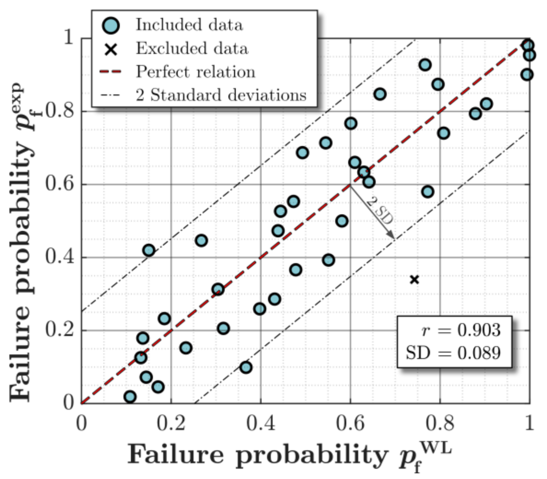
5. Evaluation of Failure Probability and Determination of Model Parameters

For each specimen, the simulated stress distribution for the clamping phase and the cyclic loading are used to determine the distribution of the maximum principal stress amplitude at the weld surface. The failure probability for the specimen is calculated by writing the area integral in Equation (6) into a double integral

$$s_{\mathrm{equ}} = {\left[\frac{1}{A_{\mathrm{ref}}}\int \int s_{\mathrm{eff}}{\left(\eta ,\xi \right)}^{\beta }d\xi d\eta \right]}^{\frac{1}{\beta }},$$

(9)

where the first integration direction, $\xi$, is along the weld profiles and the second integration direction, $\eta$, is in the scanning direction. This is presented schematically in Figure 9. The integral is evaluated numerically as

$$s_{\mathrm{equ}} = {\left[\frac{1}{A_{\mathrm{ref}}}{\displaystyle \sum }_i{\displaystyle \sum }_j{s}_{\mathrm{eff}}\left({\eta }_i,{\xi }_j\right)\Delta {\xi }_j\Delta {\eta }_j\right]}^{\frac{1}{\beta }},$$

(10)

where ${\eta }_i$ and ${\xi }_j$ are the nodal positions and $s_{\mathrm{eff}}\left({\eta }_i,{\xi }_j\right)$ is the effective stress value evaluated at the corner nodes. The latter is computed by extrapolation of the stress values from the Gauss points, followed by an averaging at each node.

The two model parameters, $\beta$ and ${\lambda }_0$ in Equations (4) and (5), are fitted by minimising the mean square error ($MSE$) given by

$$MSE = \frac{1}{n_{\mathrm{spec}}}{\displaystyle \sum }_{i = 1}^{n_{\mathrm{spec}}}{\left(p_{\mathrm{f},i}^{\exp } - p_{\mathrm{f},i}^{\mathrm{WL}}\right)}^2.$$

(11)

The parameters that minimised the $MSE$ are presented in Table 2. One specimen was excluded from the fitting process as it singly influenced the fitted parameters and increased the MSE more than any other specimen. The same specimen after the fitting was verified as an outlier as it was more than 1.5 times the interquartile range [42] away from the upper quartile or below the lower quartile of the relative error in estimated failure probability

$$e_i = \left|p_{\mathrm{f},i}^{\exp } - p_{\mathrm{f},i}^{\mathrm{WL}}\right|.$$

(12)

The parameter $e_i$ is the fitting error of the Weakest-link model. The fitting accuracy is quantified using Pearson’s correlation coefficient

$$r = \frac{n_{\mathrm{spec}}\sum p_{\mathrm{f},i}^{\exp }{p}_{\mathrm{f},i}^{\mathrm{WL}} - \sum p_{\mathrm{f},i}^{\exp }\sum p_{\mathrm{f},i}^{\mathrm{WL}}}{\sqrt{n_{\mathrm{spec}}\sum {\left(p_{\mathrm{f},i}^{\exp }\right)}^2 - {\left(\sum p_{\mathrm{f},i}^{\exp }\right)}^2}\sqrt{n_{\mathrm{spec}}\sum {\left(p_{\mathrm{f},i}^{\mathrm{WL}}\right)}^2 - {\left(\sum p_{\mathrm{f},i}^{\mathrm{WL}}\right)}^2}}$$

(13)

and is presented together with the root mean square error $RMSE=\sqrt{MSE}$ in

Table 3. Fitting parameters and accuracy metrics.

Weakest-Link Fitting Parameters		Accuracy Metrics
β (-)	λ0 (MPa)	$RMSE$	r
8.22	314	0.121	0.903

. The fitting accuracy of each specimen is presented in Figure 12 where the model failure probabilities are compared with the experimental values derived from the median rank approximation. A high correlation of 0.9 is computed between experimental and model failure probability. Therefore, the proposed modelling approach captures the influence of weld topography on the specimen fatigue failure probability well.

6. Influence of Sampling Resolution on Predicted Fatigue Failure Probability

In the following, the Weakest-link model is implemented using different sampling resolutions and sampling sequences, in order to quantify the sampling-induced uncertainty. Based on the quantified uncertainty, an optimal sampling resolution is thereafter recommended.

6.1. Sampling-Induced Uncertainty in Computed Fatigue Failure Probability

Consider the weld geometry of the specimen shown in Figure 12, which is scanned using a high resolution of 50 μm. The geometry of the specimen is resampled with lower sampling resolutions and different sampling sequences, as schematically shown in Figure 13. As can be seen, each sampling sequence corresponds to a different scanning start position. By taking every other weld profile into consideration, the sampling resolution is decreased to 100 μm with two possible starting positions. Decreasing the sampling resolution further to every fourth weld profile decreases the resolution to 200 μm with four possible starting positions. It is noted that that the highest sampling resolution of 50 μm corresponds to 1200 weld profiles for the studied 60 mm long weld.

The weld geometry of the specimen is scanned from the different scanning starting positions using a sampling resolution of 50, 100, 200, 250, 500, 1000, 2000 and 5000 μm. This corresponds to more than 100 scanned weld surfaces with different combinations of sampling resolutions and scanning start positions. An FE simulation is thereafter performed for each of the scanned surfaces and the failure probability is computed using Equation (9). The computed failure probabilities for different sampling starting positions are presented in Figure 14a–e for each sampling resolution. In Figure 14a, the failure probabilities for four different scanning start positions are shown. These four start positions are illustrated in Figure 13 for a resolution of 200 μm (start positions 1, 2, 3 and 4). If the resolution is reduced by a factor of 10, see Figure 14c, a total of 40 different scanning start positions results in the shown variation in the computed failure probability. As can be seen, the computed failure probability appears to have a sinusoidal relation to the scanning start position. It is noted that all probabilities are computed at $n=\mathrm{761,384}$ cycles, which is the experimental number of cycles to failure for the considered specimen.

6.2. Required Sampling Resolution

To determine the required scanning accuracy, all computed probabilities in Figure 14a–f are plotted as a function of the sampling resolution, see Figure 15a. For each resolution, the marked crosses correspond to different scanning start positions as described in Figure 13. The mean and variance of the failure probability are determined for each sampling resolution as

$${\overline{p}}_{\mathrm{f}}^{\mathrm{WL}} = \frac{1}{n_{\mathrm{seq}}}{\displaystyle \sum }_{j = 1}^{n_{\mathrm{seq}}}{p}_{\mathrm{f},j}^{\mathrm{WL}}$$

(14)

And

$$\mathrm{Var}\left[p_{\mathrm{f}}^{\mathrm{WL}}\right] = \sqrt{\frac{1}{n_{\mathrm{seq}}}{\displaystyle \sum }_{j = 1}^{n_{\mathrm{seq}}}\left(p_{\mathrm{f},j}^{\mathrm{WL}} - {\overline{p}}_{\mathrm{f}}^{\mathrm{WL}}\right)}$$

(15)

respectively, where $p_{\mathrm{f},j}^{\mathrm{WL}}$ is the Weakest-link probability computed using a sampling sequence $j$ and $n_{\mathrm{seq}}$ is the number of sampling sequences for the considered resolution (see Figure 14). As can be seen, the standard deviation $\sqrt{\mathrm{Var}\left[p_{\mathrm{f}}^{\mathrm{WL}}\right]}$ decreases with decreasing sampling resolution. It is further noted that, although the mean probability slightly decreases with decreased resolution, this change is relatively small.

In Figure 15b, the relative error in the failure probabilities, with respect to the probability computed at the highest resolution of 50 μm, is plotted as a function of sampling resolution based on

$${\mathrm{error}}_i = \frac{\left|{\left.p_{\mathrm{f}}^{\mathrm{WL}}\right|}_{50\mathsf{\mu }\mathrm{m}} - p_{\mathrm{f},i}^{\mathrm{WL}}\right|}{{\left.p_{\mathrm{f}}^{\mathrm{WL}}\right|}_{50\mathsf{\mu }\mathrm{m}}}\times 100\%$$

(16)

It is from Figure 15b possible to determine the required sampling resolution by setting an allowable relative error. It should be noted that the tolerated uncertainty in predicted failure probability is highly dependent on the application. A higher degree of certainty is generally needed for structurally critical components in the high cycle fatigue regime. For the studied specimen, a sampling resolution of 200 to 250 μm results in an acceptable mean relative error in $p_{\mathrm{f}}$ of less than 2%.

7. Concluding Remarks

In this study, the influence of sampling resolution in digital scanning of welds for fatigue quality control was investigated. The method for determining the optimal resolution consisted of five steps.

• Digital scanning—the local weld geometries of more than 50 welded tee joints were measured with a high resolution of 50 μm.
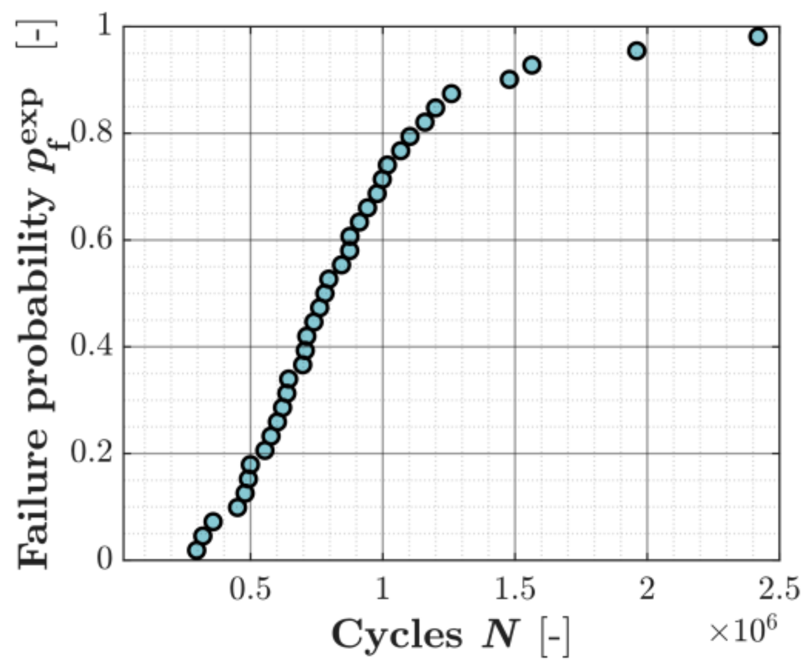
• Fatigue testing—all measured specimens were fatigue tested at the same load level. The experimental fatigue failure probability was computed using median rank for each specimen that failed within 5 million cycles.
• Finite-element analysis—for each of the failed specimens during fatigue testing, the local stresses on the weld surface were computed from FE analysis using the Digital scanning data of the weld topography.
• Weakest-link failure probability—a two-parameter weakest-link area model was applied to model the fatigue failure probability based on the local stresses computed from the finite element analysis. The weakest-link parameters were determined by fitting the model probabilities to the experimental probabilities determined from the fatigue testing.
• Sensitivity analysis—the sensitivity of the computed Weakest-link failure probability to a reduction in sampling resolution was studied based on an arbitrarily chosen specimen. The digital scanning data was down-sampled to sampling resolutions in the range of 100 μm to 5 mm with different scanning start positions. A finite-element analysis was performed for each of the down-sampled scanned geometries and the corresponding failure probability was computed. The error and uncertainty in the computed probabilities due to the down-sampling was quantified and the required sampling resolution was determined by setting an allowable mean error.

Based on the above steps, a sampling resolution of 200 to 250 μm has been shown to be adequate for fatigue quality control of the studied welded joints. This sampling resolution results in a mean relative error of less than 2% in the computed fatigue failure probability compared to highest studied resolution in this work (50 μm). The present study therefore indicates that the local weld geometry needs to be captured with a relatively high resolution to accurately predict the failure probability.

The adequate sampling resolution presented in this study would, in a production environment, be translated to scanning speeds of around 20–25 mm weld per second scanning using a high sampling frequency of 100 Hz (illustrated in Figure 3). This means that the time it would take to scan 1 m of weld is 40–50 s.

This study also suggests that a two-parameter Weakest-link area model using the maximum principal stress as a multiaxial effective stress measure, is appropriate to model the failure probability of welds. This is demonstrated by a correlation coefficient of 0.9 between model and experimental probabilities for the studied tee joints.

Finally, this work paves the way to quantifying the influence of local geometrical variations on the fatigue failure probability by combining advanced statistical spatial field analysis [43,44,45] of the scanned data and Weakest-link fatigue models. A comparison between Weakest-link area [46] and volume models [47] as well as the choice of multiaxial effective stress measure [48] need to be investigated further.

References

1. Mansour, R.; Zhu, J.; Edgren, M.; Barsoum, Z. A probabilistic model of weld penetration depth based on process parameters. Int. J. Adv. Manuf. Technol. 2019, 105, 499–514. [Google Scholar] [CrossRef] [Green Version]
2. Tomaz, I.D.V.; Colaço, F.H.G.; Sarfraz, S.; Pimenov, D.Y.; Gupta, M.K.; Pintaude, G. Investigations on quality characteristics in gas tungsten arc welding process using artificial neural network integrated with genetic algorithm. Int. J. Adv. Manuf. Technol. 2021, 113, 3569–3583. [Google Scholar] [CrossRef]
3. Jonsson, B.; Samuelsson, J.; Marquis, G.B. Development of weld quality criteria based on fatigue performance. Weld. World 2011, 55, 79–88. [Google Scholar] [CrossRef]
4. Hammersberg, P.; Technology, M.; Olsson, H. Statistical evaluation of welding quality in production. In Proceedings of the Swedish Conference on Light Weight Optimized Welded Structures, Borlänge, Sweden, 24–25 March 2010; pp. 148–162. [Google Scholar]
5. Stenberg, T.; Lindgren, E.; Barsoum, Z. Development of an algorithm for quality inspection of welded structures. Proc. Inst. Mech. Eng. Part B J. Eng. Manuf. 2012, 226, 1033–1041. [Google Scholar] [CrossRef]
6. Stenberg, T.; Barsoum, Z.; Åstrand, E.; Ericson Öberg, A.; Schneider, C.; Hedegård, J. Quality control and assurance in fabrication of welded structures subjected to fatigue loading. Weld. World 2017, 61, 1003–1015. [Google Scholar] [CrossRef] [Green Version]
7. Barsoum, Z.; Stenberg, T.; Lindgren, E. Fatigue properties of cut and welded high strength steels-Quality aspects in design and production. Procedia Eng. 2018, 213, 470–476. [Google Scholar] [CrossRef]
8. Hultgren, G.; Barsoum, Z. Fatigue assessment in welded joints based on geometrical variations measured by laser scanning. Weld. World 2020, 64, 1825–1831. [Google Scholar] [CrossRef]
9. Stasiuk, P.; Karolczuk, A.; Kuczko, W. Analysis of correlation between stresses and fatigue lives of welded steel specimens based on real three-dimensional weld geometry. Acta Mech. Autom. 2016, 10, 12–16. [Google Scholar] [CrossRef] [Green Version]
10. Alam, M.M.; Barsoum, Z.; Jonsén, P.; Kaplan, A.F.H.; Häggblad, H.Å. The influence of surface geometry and topography on the fatigue cracking behaviour of laser hybrid welded eccentric fillet joints. Appl. Surf. Sci. 2010, 256, 1936–1945. [Google Scholar] [CrossRef]
11. Lang, R.; Lener, G.; Schmid, J.; Ladinek, M. Welded seam evaluation based on 3D laser scanning—Practical application of mobile laser scanning systems for surface analysis of welds—Part 1. Stahlbau 2016, 85, 336–343. [Google Scholar] [CrossRef]
12. Lang, R.; Lener, G. Assessment of welds based on 3D laser scanning. Practical application of a mobile laser scan system for the surface assessment of welds—Part 2. Stahlbau 2016, 85, 395–408. [Google Scholar] [CrossRef]
13. Lang, R.; Lener, G. Application and comparison of deterministic and stochastic methods for the evaluation of welded components’ fatigue lifetime based on real notch stresses. Int. J. Fatigue 2016, 93, 184–193. [Google Scholar] [CrossRef]
14. Lener, G.; Lang, R.; Ladinek, M.; Timmers, R. A numerical method for determining the fatigue strength of welded joints with a significant improvement in accuracy. Procedia Eng. 2018, 213, 359–373. [Google Scholar] [CrossRef]
15. Vuherer, T.; Maruschak, P.; Samardžić, I. Behaviour of coarse grain heat affected zone (HAZ) during cycle loading. Metalurgija 2012, 51, 301–304. Available online: https://hrcak.srce.hr/8 (accessed on 30 April 2021).
16. Niederwanger, A.; Warner, D.H.; Lener, G. The utility of laser scanning welds for improving fatigue assessment. Int. J. Fatigue 2020, 140, 105810. [Google Scholar] [CrossRef]
17. Kaffenberger, M.; Vormwald, M. Fatigue resistance of weld ends—Analysis of the notch stress using real geometry. Materwiss. Werksttech. 2011, 42, 874–880. [Google Scholar] [CrossRef]
18. Kaffenberger, M.; Vormwald, M. Application ofthe notch stress concept to the real geometry ofweld end points. Materwiss. Werksttech. 2011, 42, 289–297. [Google Scholar] [CrossRef]
19. Hou, C.Y. Fatigue analysis of welded joints with the aid of real three-dimensional weld toe geometry. Int. J. Fatigue 2007, 29, 772–785. [Google Scholar] [CrossRef]
20. Hou, C.Y. Computer simulation of weld toe stress concentration factor sequence for fatigue analysis. Int. J. Struct. Integr. 2019, 10, 792–808. [Google Scholar] [CrossRef]
21. Chaudhuri, S.; Crump, J.; Reed, P.A.S.; Mellor, B.G. High-resolution 3D weld toe stress analysis and ACPD method for weld toe fatigue crack initiation. Weld. World 2019, 63, 1787–1800. [Google Scholar] [CrossRef] [Green Version]
22. Aldén, R.; Barsoum, Z.; Vouristo, T.; Al-Emrani, M. Robustness of the HFMI techniques and the effect of weld quality on the fatigue life improvement of welded joints. Weld. World 2020, 64, 1947–1956. [Google Scholar] [CrossRef]
23. Liinalampi, S.; Remes, H.; Lehto, P.; Lillemäe, I.; Romanoff, J.; Porter, D. Fatigue strength analysis of laser-hybrid welds in thin plate considering weld geometry in microscale. Int. J. Fatigue 2016, 87, 143–152. [Google Scholar] [CrossRef]
24. Ladinek, M.; Niederwanger, A.; Lang, R.; Schmid, J.; Timmers, R.; Lener, G. The strain-life approach applied to welded joints: Considering the real weld geometry. J. Constr. Steel Res. 2018, 148, 180–188. [Google Scholar] [CrossRef]
25. Ladinek, M.; Niederwanger, A.; Lang, R. An individual fatigue assessment approach considering real notch strains and local hardness applied to welded joints. J. Constr. Steel Res. 2018, 148, 314–325. [Google Scholar] [CrossRef]
26. Lang, E.; Rudolph, J.; Beier, T.; Vormwald, M. Low Cycle Fatigue Behavior of Welded Components: A New Approach—Experiments and Numerical Simulation. In Proceedings of the Pressure Vessels and Piping Conference, Toronto, ON, Canada, 15–19 July 2012; pp. 289–298. [Google Scholar]
27. Lang, E.; Rudolph, J.; Beier, H.T.; Vormwald, M. Geometrical influence of a butt weld in the low cycle fatigue regime. Procedia Eng. 2013, 66, 73–78. [Google Scholar] [CrossRef]
28. Wormsen, A.; Sjödin, B.; Härkegård, G.; Fjeldstad, A. Non-local stress approach for fatigue assessment based on weakest-link theory and statistics of extremes. Fatigue Fract. Eng. Mater. Struct. 2007, 30, 1214–1227. [Google Scholar] [CrossRef]
29. Sandberg, D.; Mansour, R.; Olsson, M. Fatigue probability assessment including aleatory and epistemic uncertainty with application to gas turbine compressor blades. Int. J. Fatigue 2017, 95, 132–142. [Google Scholar] [CrossRef]
30. Hultgren, G.; Mansour, R.; Barsoum, Z.; Olsson, M. Fatigue probability model for AWJ-cut steel including surface roughness and residual stress. J. Constr. Steel Res. 2021, 179, 106537. [Google Scholar] [CrossRef]
31. Marquis, G.B.; Barsoum, Z. IIW Recommendations for the HFMI Treatment; IIW Collection; Springer: Singapore, 2016; ISBN 9789811025037. [Google Scholar]
32. Winteria|Laser Scanning Systems for Quality Assurance. Available online: https://winteria.se (accessed on 7 April 2021).
33. Benard, A.; Bos-Levenbach, E.C. Het uitzetten van waarnemingen op waarschijnlijkheids-papier. Stat. Neerl. 1953, 7, 163–173. [Google Scholar] [CrossRef] [Green Version]
34. Hobbacher, A.F. Recommendations for Fatigue Design of Welded Joints and Components; IIW Collection; Springer International Publishing: Cham, Switzerland, 2016; ISBN 9783319237565. [Google Scholar]
35. Mansour, R.; Olsson, M. Efficient Reliability Assessment with the Conditional Probability Method. J. Mech. Des. Trans. ASME 2018, 140. [Google Scholar] [CrossRef]
36. Hasofer, A.M.; Lind, N.C. Exact and Invariant Second-Moment Code Format. ASCE J. Eng. Mech. Div. 1974, 100, 111–121. [Google Scholar] [CrossRef]
37. Mansour, R.; Olsson, M. A closed-form second-order reliability method using noncentral chi-squared distributions. J. Mech. Des. Trans. ASME 2014, 136. [Google Scholar] [CrossRef]
38. Mansour, R.; Olsson, M. Response surface single loop reliability-based design optimization with higher-order reliability assessment. Struct. Multidiscip. Optim. 2016, 54, 63–79. [Google Scholar] [CrossRef]
39. Hu, Z.; Du, X. Saddlepoint approximation reliability method for quadratic functions in normal variables. Struct. Saf. 2018, 71, 24–32. [Google Scholar] [CrossRef]
40. Park, J.W.; Lee, I. A Study on Computational Efficiency Improvement of Novel SORM Using the Convolution Integration. J. Mech. Des. Trans. ASME 2018, 140. [Google Scholar] [CrossRef]
41. Olsson, E.; Olander, A.; Öberg, M. Fatigue of gears in the finite life regime—Experiments and probabilistic modelling. Eng. Fail. Anal. 2016, 62, 276–286. [Google Scholar] [CrossRef]
42. Tukey, J.W. Exploratory Data Analysis; Addison-Wesley: Boston, MA, USA, 1977; ISBN 978-0-201-07616-5. [Google Scholar]
43. Genton, M.G.; Kleiber, W. Cross-Covariance Functions for Multivariate Geostatistics. Stat. Sci. 2015, 30, 147–163. [Google Scholar] [CrossRef]
44. Mansour, R.; Kulachenko, A.; Chen, W.; Olsson, M. Stochastic Constitutive Model of Isotropic Thin Fiber Networks Based on Stochastic Volume Elements. Materials 2019, 12, 538. [Google Scholar] [CrossRef] [Green Version]
45. Alzweighi, M.; Mansour, R.; Lahti, J.; Hirn, U.; Kulachenko, A. The influence of structural variations on the constitutive response and strain variations in thin fibrous materials. Acta Mater. 2021, 203, 116460. [Google Scholar] [CrossRef]
46. Lanning, D.B.; Nicholas, T.; Palazotto, A. HCF notch predictions based on weakest-link failure models. Int. J. Fatigue 2003, 25, 835–841. [Google Scholar] [CrossRef]
47. Tomaszewski, T.; Strzelecki, P.; Mazurkiewicz, A.; Musiał, J. Probabilistic Estimation of Fatigue Strength for Axial and Bending Loading in High-Cycle Fatigue. Materials 2020, 13, 1148. [Google Scholar] [CrossRef] [PubMed] [Green Version]
48. Norberg, S.; Olsson, M. The effect of loaded volume and stress gradient on the fatigue limit. Int. J. Fatigue 2007, 29, 2259–2272. [Google Scholar] [CrossRef]
Figure 1. Workflow of the present study.
Metals 11 00822 g001
Figure 2. Fatigue test specimen, single-pass tee joint weld specimen.
Metals 11 00822 g002
Figure 3. Sampling resolution (mm) for different combinations of scanning speeds (mm/s) and sampling frequencies (Hz).
Metals 11 00822 g003
Figure 4. (a) Weld geometry definitions and (b) variation measured by the Winteria® qWeld [32] system for specimen 24.
Metals 11 00822 g004
Figure 5. Variation of geometry within the tested group of specimens.
Metals 11 00822 g005
Figure 6. Scatter of the uniaxial fatigue test data.
Metals 11 00822 g006
Figure 7. Experimental failure probability using the median rank method.
Metals 11 00822 g007
Figure 8. (a) Measured area and (b) reference area of the welded joint used in the Weakest-link area model.
Metals 11 00822 g008
Figure 9. Structured discretisation of the weld geometry surface.
Metals 11 00822 g009
Figure 10. Boundary condition applied in the numerical simulations of the stress distribution.
Metals 11 00822 g010
Figure 11. Stress distribution at the weld surface of the specimen 24 (failure order 17 in Table 1) for a nominal stress of 180 MPa.
Metals 11 00822 g011
Figure 12. Numerical fatigue strength estimations at the corresponding fatigue life determined from experimental testing.
Metals 11 00822 g012
Figure 13. Resampling of scanning data by excluding weld profiles. Each row represents a sampled sequence including only the profiles with filled cells.
Metals 11 00822 g013
Figure 14. Influence of starting position on the model failure probability at different sampling resolutions. (a) 200 μm sampling resolution, (b) 250 μm sampling resolution, (c) 500 μm sampling resolution, (d) 1000 μm sampling resolution, (e) 2000 μm sampling resolution.
Metals 11 00822 g014
Figure 15. Influence of sampling resolution on (a) the computed Weakest-link failure probability of 1 digitally scanned specimen and (b) the relative absolute error in the computed probability with respect to the highest resolution (50 μm). At each sampling resolution, different sampling sequences are marked by crosses.
Metals 11 00822 g015