Machine Learning-Based Models for the Estimation of the Energy Consumption in Metal Forming Processes

Abstract

This research provides an insight on the performances of machine learning (ML)-based algorithms for the estimation of the energy consumption in metal forming processes and is applied to the radial-axial ring rolling process. To define the mutual influence between ring geometry, process settings, and ring rolling mill geometries with the resulting energy consumption, measured in terms of the force integral over the processing time (FIOT), FEM simulations have been implemented in the commercial SW Simufact Forming 15. A total of 380 finite element simulations with rings ranging from 650 mm < DF < 2000 mm have been implemented and constitute the bulk of the training and validation datasets. Both finite element simulation settings (input), as well as the FI (output), have been utilized for the training of eight machine learning models, implemented with Python scripts. The results allow defining that the Gradient Boosting (GB) method is the most reliable for the FIOT prediction in forming processes, being its maximum and average errors equal to 9.03% and 3.18%, respectively. The trained ML models have been also applied to own and literature experimental cases, showing a maximum and average error equal to 8.00% and 5.70%, respectively, thus proving once again its reliability.

1. Introduction

The radial axial-ring rolling (RARR) is a versatile forging process widely used in different industrial sectors such as automotive, agricultural, wind power, piping, and aerospace [1]. In recent years, several improvements have been introduced helping to obtain good surface quality, fine tolerances, and a considerable saving in material cost [2] with less production time compared to the machining process. Rings manufactured through RARR have high durability and structural strength, but the complexity of the process makes its settings and control hard to be handled without numerical simulations or prediction algorithms. For these reasons, several authors focused their attention on the development of algorithms and finite element models for a better understanding of the ring rolling process, as is hereafter summarized.

Lugora and Bramley [3] utilized Hill’s general method for predicting the evolution of the ring during the process considering a rigid-perfectly plastic and incompressible material. Bruschi et al. [4] established a real-time control model, based on the artificial neural network (ANN) approach, to predict the geometrical accuracy of the ring, showing a good correlation between the ANN model and FEM results. Guo and Yang [5] defined the steady forming condition for the ring rolling process and built a mathematical model based on a constant velocity growth condition of the ring and considered the ring geometry in terms of average diameters. More recently, Quagliato and Berti [6] superseded this limit by proposing a more accurate mathematical approach for the determination of the ring geometry for a subsection of the ring geometry, defined as a slice.

As concerns the force prediction for the ring rolling process, Quagliato and Berti [7,8] proposed two mathematical models based on the slip line theory and estimated radial and axial forces with a deviation equal to ~5% and ~6%, respectively, in comparison to the relevant FEM simulations and experimental results. Furthermore, Ryoo et al. [9] defined the relationship between the parameters that affect the ring rolling process at high temperatures and investigated the influence of the main roll rotational speed and the mandrel feeding speed. Kalyani et al. [10] investigated radial and axial forces during the forming process of profiled rings in terms of time and temperature, calculated the forces with an analytical approach, and compared them with FEM simulations. Kim et al. [11] investigated the influence of process parameters in producing large rings, focusing on minimizing the load, but did not consider temperature and process parameters’ reciprocal influence.

As concerns energy estimation and starvation algorithms for industrial process, due to the strong influence of the energy demand on production planning and control [12], several authors focused on this topic. Unver and Kara [13] introduced a decision support tool called HORUS 5.0 to determine the lowest energy-consuming route within the scope of sustainable energy efficiency. Meissner et al. [14] developed an indicator system considering the impact of the materials, energies, and economic attributes of energy efficiency, concluding that strategic decision-making concerning energy optimization is important to be competitive. Larkiola et al. [15] investigated the role of energy efficiency in the rolling processes employing an ANN-based approach and achieved an improvement estimated in 1.8% of the overall energy efficiency. Giorleo et al. [16] compared simulation analyses with an industrial case to evaluate the effect of utilizing different ring preform geometries to reduce the total energy required during the process but focused on a single material and single set of process parameters. Allegri et al. [17] defined a main roll speed law that allows maintaining a constant ring angular velocity and achieved a 35% fishtail defect reduction and a 9% energy consumption reduction.

As summarized so far, several authors developed models for the prediction of the kinematic expansion, the force, and torque but it seems that the impact of the process parameters on the energy consumption has not been thoroughly investigated in the literature. In the hot radial-axial ring rolling process, as in every metal forming process carried out at hot or warm forming conditions, a lower process force can be obtained by reducing the feeding, or the deformation, over time. On the other hand, a longer manufacturing time induces a higher temperature drop in the workpiece, which leads to an increase in the resistance to the deformation of the material. The energy integral over time can be estimated by employing numerical simulations [18,19,20,21] but, considering the complex tools-workpiece interaction in the RARR process, the computational time required for one single simulation might range between several hours and a few days.

In the literature, machine learning algorithms have been already applied to various manufacturing topics, such as for the prediction of joint strength of ultrasonic welding processes [22], to estimate the tool wear in milling operations [23], to diagnose the dimensional variation of additive manufactured parts [24], to classify the cutting phase of the natural fiber reinforced plastic composites [25] and to predict the tool life in the micro-milling process [26]. More recently, Wang et al. [27] developed a deep learning-based algorithm for the recognition of the defects in the strip rolling process, Marques et al. [28] investigated the performances of parametric and non-parametric models for the correlation of process and material variables to springback and wall thinning, Palmieri et al. [29] defined a metamodel to correlate the process parameters and key-quality indicators for the optimization of the blank-holding forces in the stamping process, and Winiczenko [30] utilized a hybrid response surface methodology combined with a genetic algorithm to simulate and optimize the friction welding parameters in AISI 1020-ASTM A536 joints.

Although ML algorithms have been applied to various manufacturing processes, they have not yet been utilized for the investigation of the influence of process, material, and geometrical parameters in metal forming processes and have not been applied yet to the RARR process. Accordingly, the research presented in this paper aims to fill this gap in the literature by investigating the influence of (i) process parameters, (ii) material properties, (iii) initial/final ring geometries, and (iv) processing conditions on energy consumption. Based on the implemented numerical simulation database, eight machine learning (ML) models have been trained and utilized for the prediction of the energy consumption during the process based on the above-mentioned (i, ii, iii, iv) parameters clusters. The mandrel forming force integral over time, (FIOT), has been utilized as the output variable in the analysis, and as response value for the training and validation of the ML algorithms. Based on the most recent applications of machine learning model, eight different models have been adopted in the research presented in this paper, namely: linear methods [31,32], the kernel methods [33,34], the ensemble methods [35,36,37], and the artificial neural network (ANN) methodology [38,39,40], respectively.

To create the dataset for the training and the validation of machine learning models, radial-axial ring rolling finite element simulations models have been implemented in the commercial software Simufact Forming 15: six ring final outer diameters, equal to 650, 800, 1100, 1400, 1700, and 2000 mm have been considered along with three different materials, largely utilized in the ring rolling process, namely the 42CrMo4 steel [4], the Inconel 718 superalloy [41], and the AA6082 (AlMgSi) aluminum alloy [42]. The material properties have been accounted for by its temperature-dependent elastic modulus and yield strength. Since the training and validation datasets have been all acquired through FE simulations, the implemented FEM model has been validated by comparing its results with a previously published once [8], showing a maximum deviation equal to 2.15% and 0.95% in the prediction of the radial forming force outer diameter of the ring.

A total of 380 numerical simulation models have been implemented and 80% of the results have been utilized for the training of the ML models, whereas the remaining 20% were for their validation. An additional validation phase has been carried out considering the previous literature experimental results published in [5,8,11]. Based on both validation phases, the Gradient Boosting method, belonging to the ensembles methods, has been shown to be able to accurately predict the force integral over time (FIOT) and is therefore considered to be the most reliable for the case of a complex thermo-mechanical forming process, such as the radial-axial ring rolling process.

2. Materials and Methods

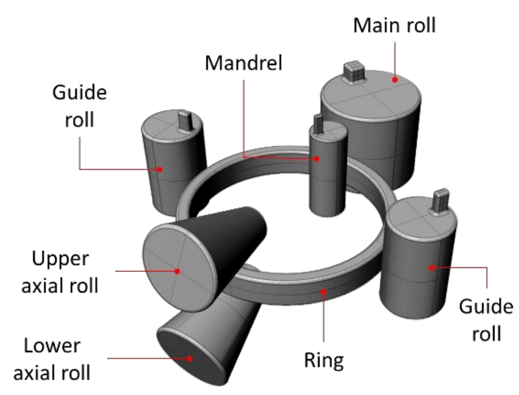
2.1. Finite Element Simulation Model Definition

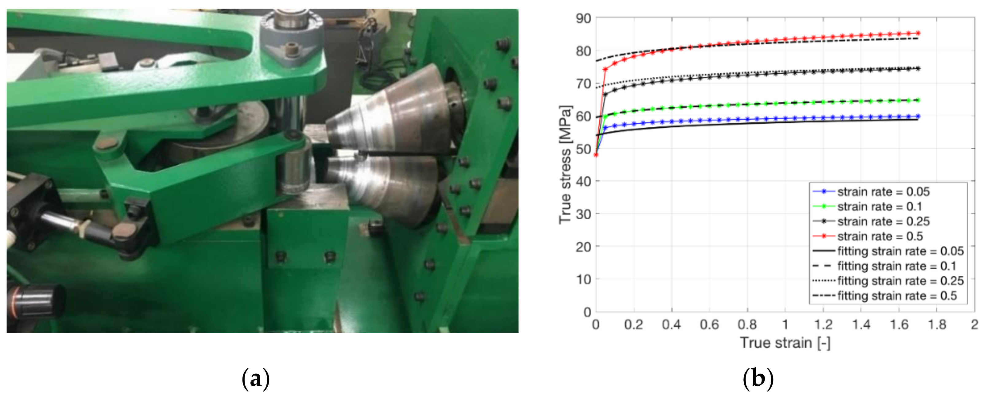
To create the database for the training of the machine learning-based force integral over time (FIOT) prediction models, presented in Section 3 of the paper, thermo-mechanical FEM simulations have been implemented in the commercial software Simufact Forming 15 following the general implementation scheme shown in Figure 1. In the numerical simulation models, the dies are considered as rigid with conductive, convective, and radiation heat transfer with the ring and the surrounding environment. The reason for introducing this approximation is justified by the fact that, although the elastic deformation in the rolls can slightly affect the final shape of the ring, its influence is negligible in comparison to the size of the rings considered in this paper. The dimensions for the tools of the ring rolling mill utilized in all the implemented FEM models are summarized in

Table 1. Ring rolling mill characteristics and general process settings.

Parameters	Values
Radius of the main roll [mm]	325
Radius of the mandrel [mm]	125
Length of the axial rolls [mm]	595.9
Half of axial rolls vertex angle [°]	17.5
Temperature of the environment [°C]	50
Tool initial temperature [°C]	150
Friction factor mandrel and main roll [−]	0.85
Friction factor axial and guide rolls [−]	0.6

along with the additional common process conditions. Friction has been modeled considering a shear friction law, Equation (1), and the utilized friction factor [6,7,8,18] is also reported in Table 1. In Equation (1), $k$ is defined as the ratio between the yield strength of the material and the square root of 3, according to the von Mises criterion.

$$\tau =m\cdot k$$

(1)

A higher friction factor has been considered for the contact conditions between the ring, mandrel, and the main roll due to higher thickness draft along the radial direction in comparison to the vertical deformation, carried out by the axial rolls. As concerns the centering rolls, their role is mainly to avoid excessive shifting of the ring during the process, thus their contact with the ring is limited and discontinuous over the processing time.

Friction influences the force calculation but, as will be shown in the results section, even though the training of the machine learning models has been carried out with a single set of friction constants (Table 1) when the model is applied to literature experimental cases, where different friction conditions are considered, an accurate FIOT prediction can still be achieved. Considering the training and validation (phase 1) datasets altogether, it is composed of 380 thermo-mechanical radial-axial ring rolling numerical simulations where the final outer diameter of the ring ($D_F$) ranges from 650 mm to 2000 mm.

As concerns the initial annular blanks, they have been defined in terms of initial outer diameter $D_0$, initial blank height $h_0$, and initial inner diameter $d_0$ according to the relevant final shape, by means of the procedure defined in Berti et al. [18]. A total of 16 different preform sizes have been utilized for the considered six final outer diameter geometries, as summarized in

Table 2. Initial and final ring geometries.

Ring Initial Geometries [mm]			Ring Final Geometries
$D_0$	$d_0$	$h_0$	$D_F$	$d_F$	$h_F$
490.5	325	188.8	650	530	180
510.9	325	156.2	650	505	145
549.3	325	112.2	650	450	100
518.9	325	195.4	800	680	180
550.9	325	175.4	800	645	155
575.3	325	218.7	1100	975	190
621.6	325	209.0	1100	930	170
621.6	325	209.0	1100	930	170
668.7	325	171.8	1100	855	122.5
876.2	600	208.2	1400	1220	180
909.3	600	221.3	1400	1190	190
897.7	600	209.4	1700	1530	170
875.7	600	226.3	2000	1875	190
944.5	600	232.4	2000	1820	180
944.7	600	232.4	2000	1820	180
1049.3	600	224.7	2000	1700	150

.

The ring preforms have been optimized considering four different mesh detail levels, and the best compromise between accuracy has been identified in (i) 1 element every 0.5° for the circumferential direction, 1 element every 2.5 mm for the radial direction, and 1 element every 5 mm for the vertical direction. These 16 geometries have been combined with different materials, Section 2.2, and process settings, Section 2.3, allowing obtaining the final database of 380 FEM simulations. Due to the impracticality of reporting the whole 380 settings in table form, a summary is added in Appendix A, whereas the whole dataset is made available as Supplementary Material.

2.2. Materials

In the FEM models, presented in the previous section, three materials largely utilized in the hot ring rolling process [4,41,42] have been considered: (i) 42CrMo4 steel, (ii) Inconel 718 super alloy and (iii) AA6082 (AlMgSi) aluminum alloy. Due to the high diversity of mechanical behaviors, the consideration of these three materials allows widening the range of validity of the proposed investigation. For the definition of the plastic material behavior, the Hansel-Spittel flow stress model [43] has been utilized, as reported in Equation (2) whereas the relevant model constant (C₁, C₂, n₁, n₂, L₁, L₂, m₁, m₂), for the three considered materials, are reported in

Table 3. Validity range and Hansel-Spittel flow stress model constants for the (i) 42CrMo4 steel, (ii) Inconel 718 super alloy and (iii) AA6082 (AlMgSi) aluminum alloy.

Parameters	42CrMo4	IN 718	AA6082
Temperature range for the model [°C]	800–1250	950–1100	200–530
Strain range for the model [[–]	0.05–2	0.05–2	0.05–0.9
Strain rate range for the model [1/s]	0.01–150	0.01–150	0.01–63
C1	5290.5	10501.1	378.5
C2	−0.00370	−0.00307	−0.00492
n1	−0.00033	−0.00018	−0.00011
n2	0.20612	0.54398	−0.02573
L1	−8.26584 × 10−5	−2.17606 × 10−5	6.03612 × 10−5
L2	0.02891	0.02376	−0.02548
m1	0.000301	−2.67316 × 10−6	0.000345
m2	−0.15618	0.09746	−0.031501

. In Equation (2), $\epsilon$, $\dot{\epsilon }$, and $T$ represent the considered strain, the strain rate, and temperature. The combined consideration of these three parameters during the FEM simulations allows estimating the flow stress of the material for each element of the mesh, thus accurately estimating the relevant forming force.

$${\sigma }_F=C_1\cdot e^{(C^2\cdot T)}\cdot {\epsilon }^{(n_1\cdot T+n_2)}\cdot e^{(\frac{L_1\cdot T+L_2}{\epsilon })}\cdot {\dot{\epsilon }}^{(m_1\cdot T+m_2)}$$

(2)

To be able to consider the influence of the material in the FIOT prediction models, the initial temperature of the ring, set as initial boundary conditions in the FEM models, as well as Young’s modulus and yield strength at that temperature, have been considered as features in the analysis. The three considered temperatures, for each one of the three materials, are reported in

Table 4. Ring rolling mill characteristics and general process settings.

Parameters	42CrMo4			IN 718			AA6082
Initial temperature [°C]	900	1050	1200	980	1025	1070	300	375	450
Density [kg/m3]	7847			8190			2695
Young modulus [GPa]	129	108	84	126	120	100	58	54	51
Yield strength [MPa]	126	50	40	216	187	161	101	82	67
Thermal conductivity [W/(m·K)]	28	29	30	29	30	31	200	208	214
Specific heat capacity [J/(kg·K)]	645	635	642	647	687	704	1032	1069	1120

along with the two above-mentioned mechanical properties. All the elastic, plastic, and thermal-mechanical properties for the three considered materials have been acquired from the MATILDA^® (Material Information Link and Database Service) database available in Simufact Forming 15.

The material features reported in Table 4 have been combined with the geometrical features, presented in previous Section 2.1, and with the process setting features, reported in the following Section 2.3, allowing the creation of the dataset utilized for the training and tests of the considered machine learning algorithms.

2.3. Radial-Axial Ring Rolling FEM Simulation Settings

The process parameters for the numerical simulations have been set considering the models proposed and validated in Berti et al. [18]. The three main parameters utilized in the analysis are reported in Equation (3), for the main roll rotational speed ${\omega }_R$, in Equations (4) and (5) for the mandrel initial ${[v_M]}_0$ and final ${[v_M]}_F$ feeding speeds, and in Equations (6) and (7) for the upper axial roll initial ${[v_A]}_0$ and final ${[v_A]}_F$ feeding speeds.

$$\frac{400}{R_R}<{\omega }_R<\frac{1600}{R_R}$$

(3)

$$\frac{{\omega }_R\cdot R_R\cdot 6.55\cdot {10}^{-3}\cdot {(R_0-r_0)}^2\cdot (\frac{1}{R_R}+\frac{1}{R_M}+\frac{1}{R_0}+\frac{1}{r_0})}{2\pi \cdot R_0}<{[v_M]}_0<\frac{{\omega }_R\cdot R_R\cdot \frac{2\cdot {\beta }_R{}^2}{{(\frac{1}{R_R}+\frac{1}{R_M})}^2}\cdot (\frac{1}{R_R}+\frac{1}{R_M}+\frac{1}{R_0}+\frac{1}{r_0})}{2\pi \cdot R_0}$$

(4)

$$\frac{{\omega }_R\cdot R_R\cdot 6.55\cdot {10}^{-3}\cdot {(R_F-r_F)}^2\cdot (\frac{1}{R_R}+\frac{1}{R_M}+\frac{1}{R_F}+\frac{1}{r_F})}{2\cdot \pi \cdot R_F}<{[v_M]}_F<\frac{{\omega }_R\cdot R_R\cdot \frac{2\cdot {\beta }_R{}^2}{{(\frac{1}{R_R}+\frac{1}{R_M})}^2}\cdot (\frac{1}{R_R}+\frac{1}{R_M}+\frac{1}{R_F}+\frac{1}{r_F})}{2\cdot \pi \cdot R_F}$$

(5)

$$\frac{{\omega }_R\cdot R_R\cdot \frac{0.0131\cdot h_0{}^2}{\left(L_0-\frac{s_0}{2}\right)\tan \left(\frac{\theta }{2}\right)}}{2\pi \cdot R_0}<{[v_A]}_0<\frac{4{\omega }_R\cdot R_R\cdot {\beta }_A{}^2\left(L_0-\frac{s_0}{2}\right)\tan \left(\frac{\theta }{2}\right)}{2\pi \cdot R_0}$$

(6)

$$\frac{{\omega }_R\cdot R_R\cdot \frac{0.0131\cdot h_F{}^2}{\left(L_F-\frac{s_F}{2}\right)\tan \left(\frac{\theta }{2}\right)}}{2\pi \cdot R_F}<{[v_A]}_F<\frac{4{\omega }_R\cdot R_R\cdot {\beta }_A{}^2\left(L_F-\frac{s_F}{2}\right)\tan \left(\frac{\theta }{2}\right)}{2\pi \cdot R_F}$$

(7)

In Equations (4) and (7) $R_R$ is the radius of the main roll, $R_M$ the radius of the mandrel, $R_0$, $r_0$, and $h_0$ the outer radius, inner radius and height of the initial ring blank, $R_F$, $r_F$, and $h_F$ the outer radius, inner radius, and height of the final ring, $\theta$ half of the axial rolls vertex angle whereas ${\beta }_R$ and ${\beta }_A$ the friction angle in the contact between main roll and mandrel and axial rolls, with the ring, respectively. The friction angle is calculated based on the friction factors, Table 1, as ${\beta }_R=arctg\left(m\right)$.

For each one of the implemented numerical simulations, the above-mentioned process parameters have been set according to the range proposed in [18] and have been considered as input for the force integral over time (FIOT) estimation models, presented in Section 4.3 of the paper. Since the process parameter setting is based on a kinematic approach, different temperatures or materials result in the same set of speeds. The summary of the implemented study cases is reported in Appendix A and is fully disclosed in the Supplementary Material.

3. Machine Learning Models Definition, Preprocessing, and Training

Due to the complex interaction between the considered process, materials, and geometry parameters, eight machine learning (ML) algorithms, one of which is based on the artificial neural network (ANN), with different levels of complexity, have been considered in this paper. The target is to implement a methodology for the estimation of the energy consumption in the radial-axial ring rolling process based on a set of input variables composed of geometry, process conditions, and materials. The architecture of the implemented ANN model is shown in Figure 2 where four hidden layers have been considered. As concerns the remaining ML models, input and output layers are the same as shown in Figure 2 but are connected through the weights vectors, defined during the optimization process. All the considered models have been applied to the above-mentioned dataset, considering 80% of the set for the model training whereas the remaining 20% has been employed for the assessment of the model accuracy. Both sets are not predetermined but are randomly selected before the training. The employed algorithms belong to the (i) linear, (ii) kernel, (iii) ensemble and (iv) artificial neural network approaches.

3.1. Linear Methods

Linear regression methods [31,32] are utilized to model linear correlations between the independent variable $x$ and dependent variable $y$ as in Equation (8). The prediction calculated by the model is defined as $\widehat{y}$ and the aim is to minimize the Residual Sum of Squares (RSS) of the objective function, as shown in Equation (9). The subscript $D$ represents the number of considered features, whereas $N$ represents the size of the dataset.

Linear methods can be expanded to model the non-linear relationships by replacing $X$ with non-linear functions. In this paper, to avoid the over-fitting problem, the regularized linear method has been utilized where constraints have been imposed on the weights vector ($\mathit{w}$) of Equation (8).

$$\widehat{y}=w_0+w_1{x}_1+\cdots +w_D{x}_D=w_0+{\mathit{w}}^{\mathrm{T}}X$$

(8)

$$\mathrm{RSS}(\mathit{w})={\displaystyle \sum _{i=1}^N(y_i-}{\mathit{w}}^{\mathrm{T}}{X}_{i,D}{)}^2$$

(9)

Based on the general form of Equation (8), the Ridge model is defined to minimize the squared sum of weights, thus resulting in the objective function ($\mathsf{\Upsilon }$), Equation (10). If the hyperparameter $\lambda$ of Equation (10) is equal to 0, we return to the original linear model of Equation (9). The hyperparameter, present in the Ridge model, as well as in other of the models subsequently presented, is a tuning parameter utilized to increase the accuracy of the prediction and is calculated, during the training, to maximize the correlation factor between independent and dependent variables [44].

$$\mathsf{\Upsilon }(\mathit{w})=\mathrm{RSS}(\mathit{w})+\lambda {\displaystyle \sum _{j=1}^D{‖w_j‖}^2}$$

(10)

Another variation of Equation (8) is defined as the Least Absolute Shrinkage and Selection Operator (LASSO) model where the absolute values of the weights are optimized to minimize the derivative of the target function $\mathsf{\Upsilon }(\mathit{w})$, defined as in Equation (11).

$$\mathsf{\Upsilon }(\mathit{w})=\frac{1}{2N}\mathrm{RSS}(\mathit{w})+\lambda {\displaystyle \sum _{j=1}^D‖w_j‖}$$

(11)

Considering together the square of the weights, as in the Ridge model of Equation (10), and the norm of the weights, as in the LASSO algorithm of Equation (11), the third considered linear model is shown as in Equation (12) and is defined as the Elastic Net model.

$$\mathsf{\Upsilon }(\mathit{w})=\frac{1}{2N}\mathrm{RSS}(\mathit{w})+\frac{1}{2}{\lambda }_2\left\{\frac{1}{2}\left(1-{\lambda }_1\right){\displaystyle \sum _{j=1}^D{‖w_j‖}^2}+{\lambda }_1{\displaystyle \sum _{j=1}^D‖w_j‖}\right\}$$

(12)

In Equation (12), if the hyperparameter is set as ${\lambda }_1=1$ then the LASSO Equation (11) is obtained, whereas if ${\lambda }_1=0$ it results in the Ridge model, respectively. The ${\lambda }_1$ and ${\lambda }_2$ parameters represent the constants related to the first and second-order norms, respectively, and are calculated based on the random search method [44].

3.2. Kernel Methods

Linear methods can be expanded to model non-linear relationships between the independent and dependent variables by replacing $X$, Equation (8), with the feature function $\varphi (x)$. The feature function can be written with the Gram matrix ($K$), as shown in Equations (13) and (14) where $\kappa (x_i,x_j)$ is the kernel function [33,34], defined to model the considered relationship. The Kernel Ridge (KR) model combines the kernel method with the Ridge model (10) and, in this paper, the polynomial kernel of Equation (15) is utilized for the Kernel Ridge model. The $c$ and $d$ constants in Equation (15) influence the feature functions and are determined through the random search method [44] during the training process.

$$\varphi \cdot \varphi {}^T=K$$

(13)

$$K=\left[\begin{array}{ccc}\kappa (x_1,x_1)& \cdots & \kappa (x_1,x_n)\\ ⋮& \ddots & ⋮\\ \kappa (x_n,x_1)& \cdots & \kappa (x_n,x_n)\end{array}\right]$$

(14)

$$\kappa (x_i,x_j)={(\gamma x_i{}^T{x}_j+c)}^d$$

(15)

Another Kernel method based on the squared norm of the weight factors is defined as the Support Vector Machine (SVM) model [45], Equation (16), where the $\mathrm{RSS}(\mathit{w})$ function of Equation (10) is changed into the epsilon intensive loss function, Equation (17). In this paper, as for the case of the SVM model, the polynomial kernel function of Equation (15) has been utilized.

$$\mathsf{\Upsilon }(\mathit{w})=C{\displaystyle \sum _{i=1}^N{L}_{\epsilon }(y_i,{\widehat{y}}_i)}+\frac{1}{2}{\displaystyle \sum _{j=1}^D{‖w_j‖}^2}$$

(16)

$$L_{\epsilon }(y,\widehat{y})=\left\{\begin{array}{ll}0& \mathrm{if}\hspace{0.17em}\left|y-\widehat{y}\right|<\epsilon \\ \left|y-\widehat{y}\right|-\epsilon & \mathrm{otherwise}\end{array}\right.$$

(17)

3.3. Ensemble Methods

The ensemble methods [35,36,37] combine different approaches and apply them to randomly selected data sub-sets to improve the prediction performances. Among the ensemble approaches, the Random Forest (RF) model, utilized in this paper, trains $M$ decision trees and calculated the response for each one of them. For each tree, the response is defined considering different intervals for the estimator, allowing the subdivision of the problem into subclasses, which are classified by their accuracy by comparing their values with the true value. The final prediction is given by the average of the $M$ ones, calculated as the average of each one relevant for each one of the subsets of every tree as shown in Equation (18) where $\widehat{y}$ is the average prediction over $M$-trees and ${\widehat{y}}_m$ is the prediction of each tree.

$$\widehat{y}={\displaystyle \sum _{m=1}^M\frac{1}{M}{\widehat{y}}_m}$$

(18)

Another ensemble method is defined as Gradient Boosting (GB) and, differently from the RF, in the beginning, only one tree ($f$) is created and it is progressively updated to minimize the objective function $\mathsf{\Upsilon }(\mathit{w})$, Equation (19). Therefore, the $m+1$ tree is based on the results of the $m$ tree compensated by the gradient residual of the previous tree by considering the learning rate $\eta$, as shown in Equation (20).

$$\mathsf{\Upsilon }(\mathit{w})=L_{\delta }(y,f)=\left\{\begin{array}{l}\frac{1}{2}{(y-f)}^2\mathrm{if}\left|y-f\right|<\delta \\ \delta \left|y-f\right|-\frac{1}{2}{\delta }^2\mathrm{otherwise}\end{array}\right.$$

(19)

The learning rate $\eta$ is defined as the speed by which the algorithm minimizes the loss function, $L_{\delta }$ for the ensemble methods and is present only for the case of ensemble and ANN methods. For the case of the linear method, like those of Section 3.1 and Section 3.2, the learning rate is not considered since the optimized value is defined as the minimum of the loss function.

$$\begin{array}{l}{f}_{m+1}=f_m+\eta \cdot r_{m+1}\\ \mathrm{where}\hspace{1em}{r}_{i,m+1}=-{\left|\frac{\partial L_{\delta }(y_i,f_i)}{\partial f_i}\right|}_{f_m}\end{array}$$

(20)

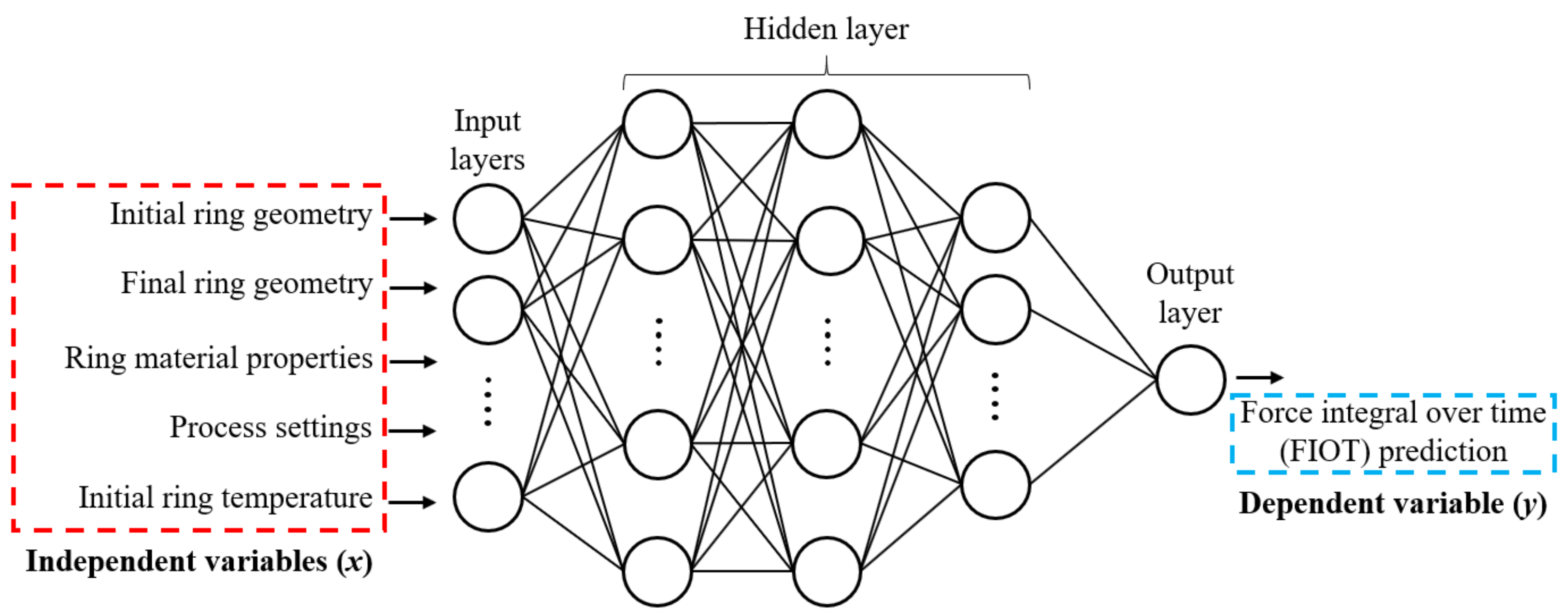
3.4. Artificial Neural Network Methods

Artificial Neural Network (ANN) models [38,39,40] consist of: (i) input layers, (ii) hidden layers, and (iii) output layers, Figure 2. Input layers are connected to the hidden layers by the weight functions ($w_{ij}$) which are calculated during the training of the ANN algorithm. For each one of the nodes, the input coming from the previous layer is defined as $x_{ij}$ and are multiplied by the weight functions ($w_{ij}$) and summed out to the bias values ($w_{i0}$), and the output of the layer is derived through the activation function ($\mathsf{\Psi }$), Equation (21).

$${\widehat{y}}_i=\mathsf{\Psi }\left({\displaystyle \sum _{j=1}^D{w}_{ij}\cdot x_j}+w_{i0}\right)$$

(21)

In the research presented in this paper, the weight matrix is updated considering the RMSprop algorithm [46], reported in Equation (22). The learning rate $\eta$ and the hyperparameter $\rho$ are optimized considering the random search method [44]. Finally, the activation function for the ANN algorithm, $\mathsf{\Psi }$ of Equation (23), is defined as the threshold for the activation of a considered node in the hidden layers.

Only if $\mathsf{\Psi }$ exceeds the threshold, the considered node in the i-layer is connected to the nodes of the i + 1 layer. The considered ANN algorithm is composed of four hidden layers made up of 200, 100, 50, and 25 nodes, respectively. The number of neurons for each layer has been optimized to minimize the loss function. The $L_{\delta }$ target function of Equation (19) has also been utilized for the case of the ANN model.

$$\begin{array}{l}{w}_{i+1}=w_i-\eta \frac{1}{\sqrt{h}}\cdot \frac{\partial L_{\delta }(y_i,{\widehat{y}}_i)}{\partial w_i}\\ \mathrm{where}\hspace{1em}{h}_i=\rho \cdot h_{i-1}+\hspace{0.17em}(1-\rho ){\left(\frac{\partial L_{\delta }(y_i,{\widehat{y}}_i)}{\partial w_i}\right)}^2\end{array}$$

(22)

$$\mathsf{\Psi }(x)\hspace{0.17em}=\hspace{0.17em}\left\{\begin{array}{c}0\hspace{1em}for\hspace{1em}x\le 0\\ x\hspace{1em}for\hspace{1em}x>0\end{array}\right.$$

(23)

3.5. Data Preprocessing and Machine Learning Algorithm Training

For the training of the selected machine learning algorithms, presented in Section 3.1, Section 3.2, Section 3.3 and Section 3.4, the input data for the 380 FEM simulations as well as the result, in terms of radial forming force integral over the mandrel time (FIOT), have been randomly arranged to avoid any bias. In both the training and test datasets, a single feature is defined as a row of the table composed of the following data: (i) main roll rotational speed, (ii) average mandrel feeding speed, (iii) initial ring geometry, (iv) final ring geometry, (v) initial ring temperature, (vi) material yield strength, (vii) material Young’s modulus and (viii) force integral over the mandrel time. Since the parameters considered in this research have different intervals and measurement units, normalization has been applied to convert them to a 0 to 1 range. As concerns the FIOT, due to the skewness of the data distribution, the input data has been converted into log(1 + FIOT) before the normalization process. Similarly, the remaining parameters have also been converted by a box-cox transformation defined as $\left(x^{0.15}-1\right)/0.15$, where x is the considered parameter.

This procedure allows reducing the computational burden during the training as well as increasing the accuracy. The hyperparameters of the prediction models described in chapter 3 have been obtained by applying the random search method aiming to maximize the correlation factor on both the training and the test datasets. The algorithms presented in the previous sections of chapter 3 have been implemented in a Windows OS environment utilizing the scikit-learn 0.22.2 and Keras 2.3.1 modules implemented in the Anaconda Spyder program with Python 3.7.4. As previously mentioned, 80% of the dataset, corresponding to 304 data, has been randomly selected from the whole database and the remaining 20%, 76 data, has been utilized as a test set.

For the evaluation of the accuracy of each model, three validation steps have been considered: (i) in the first step, the training dataset is fed once again to the model after the hyperparameters, if present, have been optimized; (ii) the test set is fed to the model and the accuracy, for the case of untrained data, is evaluated; (iii) finally, experimental values from reference papers and self-developed experiments are fed to the model and its accuracy is defined. The results concerning the accuracy of each of the considered methods, for the above-mentioned three validation steps, are reported in Section 4 of the paper along with the relevant optimized hyperparameters.

4. Results

To condense the vast amount of data relevant for the 380 numerical simulations composing the training and test datasets, the key results of three numerical simulations, in terms of equivalent plastic strain and mandrel force, have been summarized in Section 4.1. In addition to that, to prove the reliability of the numerical model implementation procedure, in Section 4.2 a validation has been carried out by comparing the outer diameter expansion and mandrel force over time. The results presented in Section 4.2 are from the authors’ previous work [8] and have been briefly summarized.

Finally, in Section 4.3, the results of the optimization of the hyperparameters as well as the performances of the considered machine learning models, as presented in Section 3, are reported. To enhance the validation of the proposed FIOT estimation procedure, the four most accurate machine learning models, among the eight employed, have been utilized for the prediction of three experimental cases from literature papers. This second validation phase allowed confirming the reliability of the defined investigation procedure as well as the accuracy of the implemented solutions.

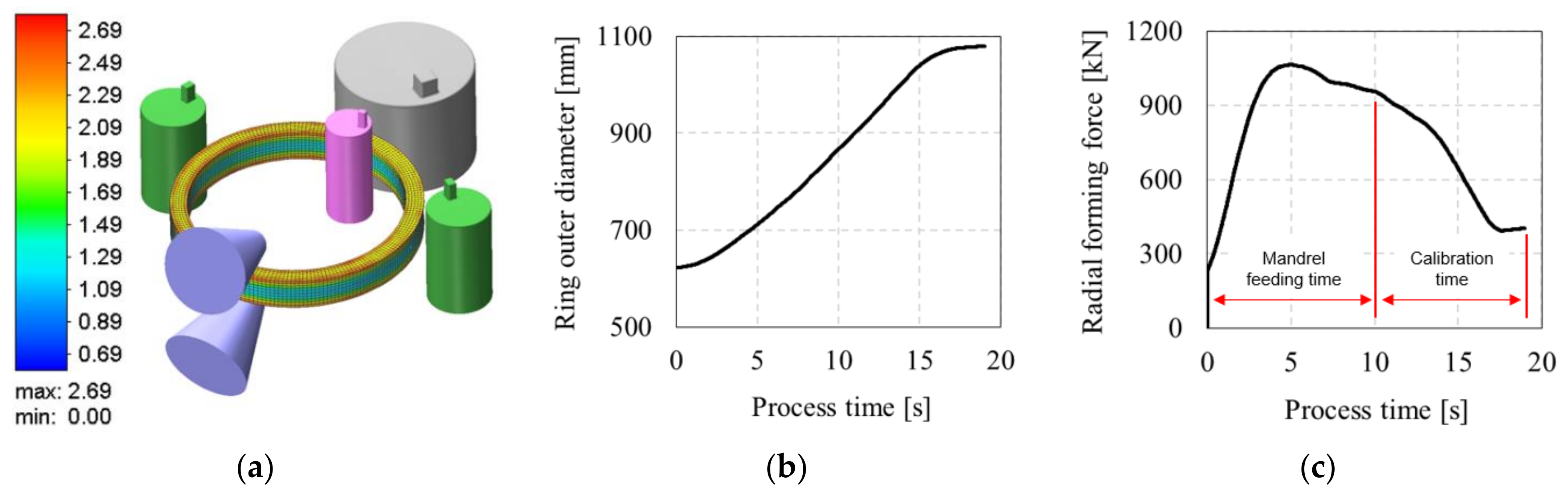
4.1. Thermo-Mechanical FEM Models Results

To provide insight on the results of the numerical simulation implemented for all the 380 analyzed cases, in Figure 3 the equivalent plastic strain distribution at the end of the calibration phase, the outer diameter, and radial force evolution during the process are reported for the case of an 1100 mm final outer diameter ring made of 42CrMo4 steel with an initial temperature of 1200 °C. The radial (mandrel) forming forces relevant for all the 380 cases have been exported from the FEM simulations and utilized for the creation of the training and test database for the machine learning algorithms. Due to the large amount of data composing the database, they are not included in the manuscript but submitted along with the paper as Supplementary Material.

After the export of the results of the radial forming force from the Simufact Forming 15 numerical simulations, a script has been implemented in MS-Excel for the automatic calculation of the time integral of the force, allowing to calculate the FIOT, utilized as a sort of measure of the amount of energy required in the whole forming process.

For the calculation of the FIOT, only the mandrel time, Figure 3c, utilized as user input in the numerical simulation, has been considered. The overall simulation time is composed of mandrel time and calibration time but, since the latter one can be extended at will to increase the accuracy of the ring geometry, it has not been considered in the analysis. The mandrel time instead is the time during which the mandrel is actively translating towards the main roll, thus when most of the process energy is employed.

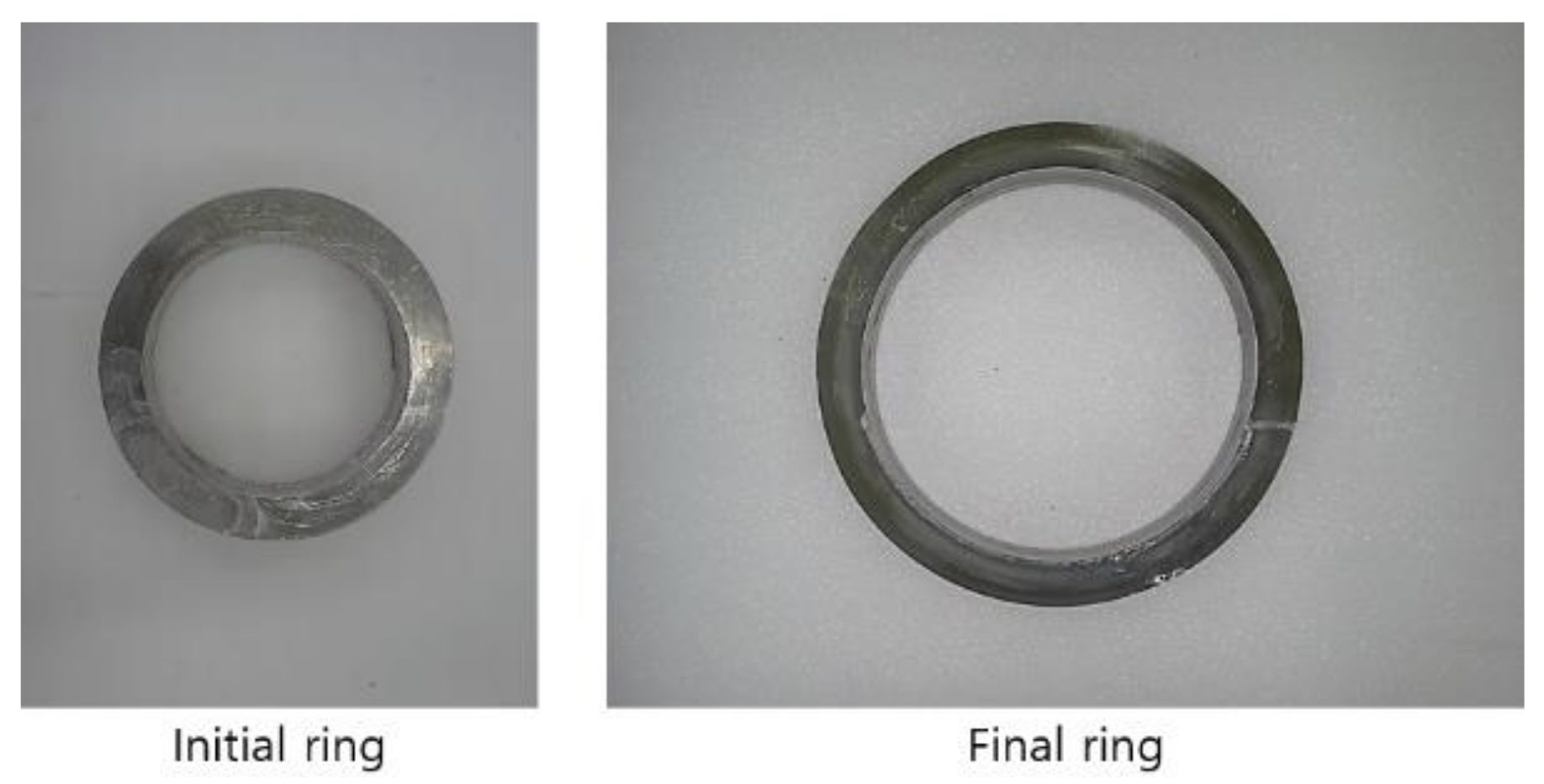
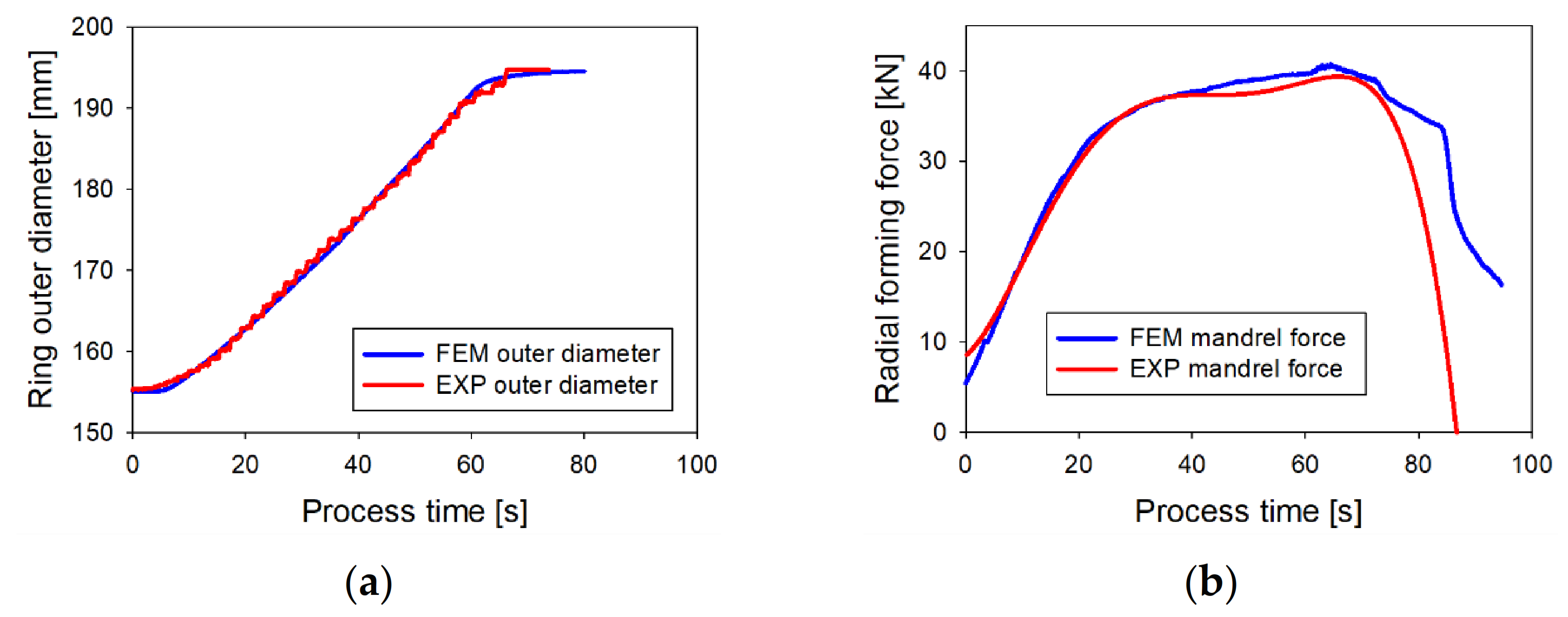
4.2. Thermo-Mechanical FEM Model Validation

To validate the developed numerical simulation model, the experimental results presented in the authors’ previous research [8] have been utilized and are hereafter summarized. For the validation, a Pb75-Sn25 alloy has been utilized for the manufacturing of the ring preform with the initial dimensions $D_0$, $d_0$ and $h_0$ equal to 155 mm, 105 mm, and 42 mm, and final dimensions equal to $D_F$, $d_F$ and $h_F$ equal to 195 mm, 153 mm, and 37 mm, respectively (Figure 4).

Additional details concerning the material properties of the Pb75-Sn25 and the ring rolling machine utilized for the validation experiments are reported in Appendix B of the paper. The validation of the implemented thermo-mechanical finite element simulation has been carried out by comparing numerical and experimental results relevant for the expansion of the outer diameter of the ring during the process, Figure 5a, and of the mandrel forming force, Figure 5b.

According to the results presented in Figure 5, the maximum deviation between experimental and finite element results is equal to 0.95% for the outer diameter 2.15% for the radial forming force, showing the reliability of the implemented numerical simulation model in replicating real process conditions. Since the FIOT estimation is based on the precise estimation of the forming force for the whole mandrel feeding time, the validation carried out against experimental results allows confirming the accuracy of the implemented finite element model solution, and thus the reliability of the input dataset for the training of the considered machine learning models.

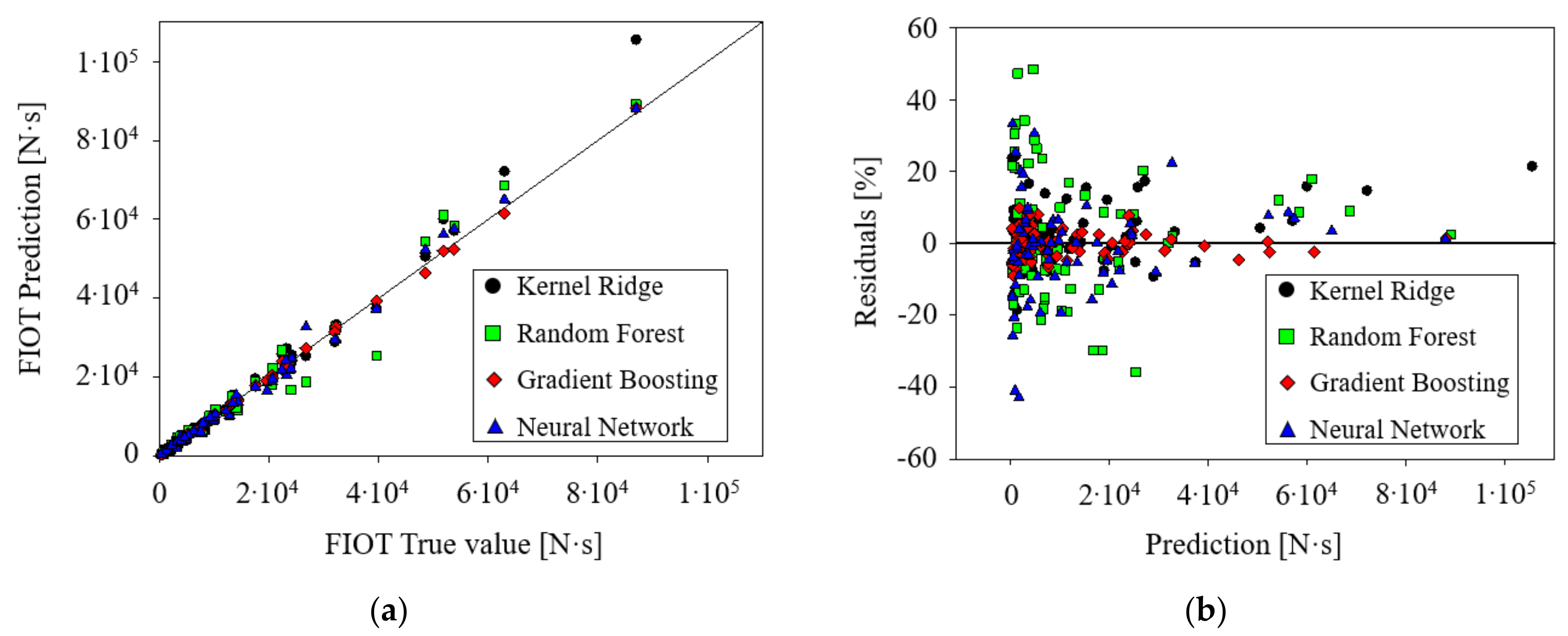
4.3. Energy Prediction Models Results and Validation

By considering the setting parameters and FIOT results of the 380 implemented FEM simulations, as presented in Section 2, the hyperparameters relevant for the eight considered machine learning models have been calculated by means of the random search method and optimized during the training phase of the algorithms. The hyperparameters have been all set as random numbers at the beginning of the training process and optimized during the training to minimize the residual between prediction and true values. During the training phase, 80% of the whole 380 simulations have been utilized and this set is defined as the “train set”. After the optimization of the hyperparameters, the trained machine learning models have been applied to the remaining 20% of the 380 simulations, not utilized during the training, and the accuracy in the estimation of the FIOT has been investigated. The accuracy of the training process has been verified by considering the correlation factor (R2). The optimized hyperparameters as well as the correlation factors for each model, relevant for the training dataset and the test dataset, calculated for the optimized hyperparameters, are reported in

Table 5. Machine learning models’ optimized hyperparameters and accuracy.

Model		Hyperparameters Values	Correlation Factor (R2)
			Train Set	Test Set
Linear method	Ridge	$\lambda =0.6$	0.920	0.855
	Lasso	$\lambda =0.0005$	0.921	0.852
	Elastic Net	${\lambda }_1=0.0005,{\lambda }_2=0.9$	0.953	0.921
Kernel method	Kernel Ridge	$\begin{array}{l}\lambda =0.02,\gamma =1.0\\ d=3.0,c=15.0\end{array}$	0.985	0.970
	Support Vector Machine	$\begin{array}{l}C=0.89,\epsilon =0.03\\ \gamma =1.0,d=3.0,c=15.0\end{array}$	0.983	0.952
Ensemble method	Random Foresting	$M=5000$	0.995	0.971
	Gradient Boosting	$\begin{array}{l}M=6900,\delta =0.9\\ \eta =0.091\end{array}$	0.998	0.996
Artificial Neural Network method	Artificial Neural Network (ANN)	$\begin{array}{l}\delta =1.0\\ \eta =0.001\end{array}$	0.993	0.992

.

According to the results presented in Table 5, the Gradient Boosting method shows the best correlation factor (R²) both in the training and test datasets. This high accuracy is related to the capability of the ensemble methods to subdivide the training dataset into sub-problems and thus, as concerns the research presented in this paper, to properly interpret the influence of different levels of the process, material, and geometrical parameters on the FIOT. Moreover, the higher accuracy of the Gradient Boosting method in comparison to the Random Forest method is related to the nature of the error minimization of the former. For the case of the Gradient Boosting method, only one tree is considered, and it is progressively optimized to minimize the residuals. The Random Forest method instead creates several trees and assigns a sub-problem to each one of them, optimizing the solutions for each one of them. However, the subdivision into sub-classes might lead to biases during the training process, a fact which is clear from the drop of the correlation factor between train test and test set for the case of the Random Forest method (Table 5).

To provide a more comprehensive evaluation of the performances of the four machine learning models that have shown the best results in terms of correlation factors (Table 5), the true values vs. prediction as well as the percentage residuals for the 76 cases of the test set are reported in Figure 6a,b, respectively. The true values in Figure 6a are the FEM result whereas the prediction values refer to the relevant ML models predictions.

The analysis of the residuals, Figure 6b, shows that although the Kernel, Random Forest and ANN methods have a remarkably high correlation factor, their residuals are considerably high, especially for small prediction values. On the other hand, the Gradient Boosting method allows having low residuals for all FIOT levels. The maximum and average residuals, for the four methods summarized in Figure 6, are reported in

Table 6. Machine learning models accuracy for the test data set.

Model	Maximum Residual	Average Residual
Kernel Ridge	24.28%	6.93%
Random Forest	48.44%	13.08%
Gradient Boosting	9.03%	3.18%
Artificial Neural Network	43.00%	9.17%

.

In addition to that, as previously mentioned, the accuracy in the prediction of the FIOT has also been evaluated for the case of three experimental ring rolling cases from the literature [5,8,11] by applying the four trained machine learning models that showed the highest correlation factors (Table 6). These experimental results are all relevant for experiments carried out on GH4169 nickel-based superalloy [5], the Pb-Sn alloy ring also utilized for the finite element model validation [8], and AISI-304 steel alloy [11]. All these three cases are completely different in terms of the geometry and material of the ring, process conditions, and size of the ring rolling mill and have been selected to provide additional insight into the accuracy of the predictions carried out by the proposed models. True prediction percentage residuals for these three cases are summarized in

Table 7. Machine learning models accuracy for the literature experimental cases.

Model	[5] FIOT Prediction Error	[8] FIOT Prediction Error	[11] FIOT Prediction Error
Kernel Ridge	16.73%	15.11%	28.97%
Random Forest	8.48%	13.44%	24.10%
Gradient Boosting	7.01%	2.09%	8.00%
Artificial Neural Network	7.23%	6.27%	9.11%

.

Considering the results presented in Table 7, it is once again clear that the structure of the Gradient Boosting method can catch the complex nature of the interaction between geometrical, material, and process parameters in the radial-axial ring rolling process thanks to its ability to subdivide the given task into sub-problems but while keeping error minimization linked to a single residual function. Moreover, as mentioned in Section 2.1, although the process conditions relevant for the [5,8,11] are different from those utilized in the FEM simulations utilized for the training, where the same friction conditions have been considered in all the cases, the accuracy is still remarkably good and the computational time is almost real-time, allowing a considerable improvement in comparison to the computational time of the thermo-mechanical numerical simulations, which may range from 9~12 h, for the case of the 650 mm final ring outer diameter simulations, to 1.5 to 3 days for the case of 2000 mm final ring outer diameter simulations.

5. Discussion

Considering the results relevant for all the utilized machine learning models, as presented in Table 5, the relatively low correlation factor shown by the linear models is an indication of the fact that the relationship between the considered input and output parameters is not linear. For the same reason, the Kernel methods, which utilize a polynomial function, show better accuracy than the linear methods but still have high residuals, as shown in the detailed analysis of Figure 6 and Table 6.

Both linear and Kernel methods calibrate the components of the weights vector ($\mathit{w}$), Equation (8) by minimizing the residual of the objective function, thus they tend to show low residuals for the case of the training dataset but relatively high ones for untrained data. On the other hand, both the Gradient Boosting as well as the Neural Network algorithms calibrate the components of the weights vector ($\mathit{w}$) considering the learning rate which allows a more robust consistency in both training and test datasets, as well as for additional predictions. Considering altogether the three validation steps carried out considering the (i) training dataset, (ii) the test dataset and (iii) the literature experimental cases, the complex interaction between process, material, and geometry parameters is therefore representable neither by a linear nor by a polynomial function.

As concerns the applicability of the proposed procedure outside the ranges considered for the construction of the training dataset, the validation case relevant for [5] gives a remarkably interesting insight. Although geometry, process parameters, and material are all different in comparison to those considered in this paper, the robustness of the trained Gradient Boosting model allows obtaining a reasonable residual in the estimation of force integral, as shown in Table 7. On the other hand, as previously mentioned, the linear and polynomial correlations considered by the linear and Kernel methods render their prediction to be affected by a high residual if the requested prediction is outside the trained ranges. Furthermore, the choice of normalizing all the parameters is also an important step for the application of the proposed procedure outside its training ranges.

Finally, an interesting feature relevant to the machine learning methods concerns the balance of the training dataset. In the considered research, the amount of data relevant for low FIOT is considerably higher than that of high force integral, and, for the case of multivariable regression methods, this fact would have resulted in good predictions for the former scenario and bad for the latter one. In principle, the need for a balanced training dataset is also valid for the machine learning models but, for the case of the ensemble methods, as well as the neural network, their sensitivity to the data clustering is almost negligible and is therefore suitable for the application in sparse and not balanced data environments. Considering altogether the investigation proposed in this paper, the applicability of the machine learning-based algorithm for the prediction of energy consumption, measured in terms of force integral over time, in forming processes has been largely explored, and both the results and analysis reported in this paper might be helpful for the extension of its application to additional industrially relevant processes.

6. Conclusions

The research presented in this paper highlighted the importance of considering the material, geometrical, and process parameters when estimating the forming force during the radial-axial ring rolling process. Moreover, eight different Machine Learning-based algorithms have been utilized for the prediction of the mandrel force integral over time (FIOT) and showed that the Gradient Boosting (GB) algorithm, belonging to the ensemble methods, grants the best accuracy in the prediction of the FIOT, being the maximum residual equal to 9.03%. Since the validation has been carried out on previously published results where ring geometries, process conditions, and materials were not included in the training dataset, the proposed approach has proven its robustness in predicting the FIOT also outside the range of the training data set. The trained GB algorithm can be directly applied to the radial-axial ring rolling (RARR) process through the algorithm provided as Supplementary Material and applies also to other forming and forging processes where the contact between workpiece and tools is defined by a curved line, as in the RARR process. The application of the proposed procedure allows a significant reduction in the time required for the estimation of the energy consumption during forming processes, its calculation being almost real-time, in comparison to the case of FEM simulations where the computational time ranges between ~10 h (for 650 mm final outer diameter rings) to 3 days (for 2000 m final outer diameter rings). The procedure presented in this paper can also be extended to different metal forming and forging processes by considering the same geometry, material, and process parameters influence on the energy consumption, but the creation of a new training dataset might be required. For these reasons, the research presented in this paper might be of interest to researchers and process engineers interested in energy consumption in metal forming processes.

References

1. Kim, N.; Machida, S.; Kobayashi, S. Ring rolling process simulation by the three dimensional finite element method. Int. J. Mach. Tools Manuf. 1990, 30, 569–577. [Google Scholar] [CrossRef]
2. Eruc, E.; Shivpuri, R. A summary of ring rolling technology-1. Recent trends in machines, process and production lines. Int. J. Mach. Tools Manuf. 1992, 32, 379–398. [Google Scholar] [CrossRef]
3. Lugora, C.F.; Bramley, A.N. Analysis of spread in ring rolling. Int. J. Mech. Sci. 1987, 29, 149–157. [Google Scholar] [CrossRef]
4. Bruschi, S.; Casptto, S.; Dal Negro, T.; Bariani, P.P. Real-time prediction of geometrical distortions of hot-rolled steel rings during cooling. CIRP Ann. Manuf. Technol. 2005, 54, 229–232. [Google Scholar] [CrossRef]
5. Guo, L.; Yang, H. Towards a steady forming condition for radial-axial ring rolling. Int. J. Mech. Sci. 2011, 53, 286–299. [Google Scholar] [CrossRef]
6. Quagliato, L.; Berti, G.A. Mathematical definition of the 3D strain field of the ring in the radial-axial ring rolling process. Int. J. Mech. Sci. 2016, 115–116, 746–759. [Google Scholar] [CrossRef]
7. Quagliato, L.; Berti, G.A. Temperature estimation and slip-line force analytical models for the estimation of the radial forming force in the RARR process of flat rings. Int. J. Mech. Sci. 2017, 123, 311–323. [Google Scholar] [CrossRef] [Green Version]
8. Quagliato, L.; Berti, G.A.; Kim, D.; Kim, N. Slip line model for forces estimation in the radial-axial ring rolling process. Int. J. Mech. Sci. 2018, 138–139, 17–33. [Google Scholar] [CrossRef]
9. Ryoo, J.S.; Yang, D.Y.; Johnson, W. The influence of process parameters on torque and load in ring rolling. J. Mech. Work. Technol. 1986, 12, 307–321. [Google Scholar] [CrossRef]
10. Kalyani, A.; Anand, M.; Amol, D. The Effect of Force Parameter on Profile Ring Rolling Process. Int. J. Eng. Res. 2015, V4, 840–844. [Google Scholar]
11. Kim, N.; Kim, H.; Jin, K. Optimal design to reduce the maximum load in ring rolling process. Int. J. Precis. Eng. Manuf. 2012, 13, 1821–1828. [Google Scholar] [CrossRef]
12. Roesch, M.; Lukas, M.; Schultz, C.; Braunreuther, S.; Reinhart, G. An approach towards a cost-based production control for energy flexibility. Procedia CIRP 2019, 79, 227–232. [Google Scholar] [CrossRef]
13. Unver, U.; Kara, O. Energy efficiency by determining the production process with the lowest energy consumption in a steel forging facility. J. Clean. Prod. 2019, 215, 1362–1370. [Google Scholar] [CrossRef]
14. Meißner, M.; Massalski, L.; Wirtz, A.; Wiederkehr, P.; Myrzik, J. Representation of energy efficiency of energy converting production processes by process status indicators. Procedia CIRP 2019, 79, 221–226. [Google Scholar] [CrossRef]
15. Larkiola, J.; Myllykoski, P.; Korhonen, A.S.; Cser, L. The role of neural networks in the optimisation of rolling processes. J. Mater. Process. Technol. 1998, 80–81, 16–23. [Google Scholar] [CrossRef]
16. Giorleo, L.; Ceretti, E.; Giardini, C. Energy consumption reduction in Ring Rolling processes: A FEM analysis. Int. J. Mech. Sci. 2013, 74, 55–64. [Google Scholar] [CrossRef]
17. Allegri, G.; Giorleo, L.; Ceretti, E.; Giardini, C. Driver roll speed influence in Ring Rolling process. Procedia Eng. 2017, 207, 1230–1235. [Google Scholar] [CrossRef]
18. Berti, G.A.; Quagliato, L.; Monti, M. Set-up of radial–axial ring-rolling process: Process worksheet and ring geometry expansion prediction. Int. J. Mech. Sci. 2015, 99, 58–71. [Google Scholar] [CrossRef]
19. Davey, K.; Ward, M.J. A practical method for finite element ring rolling simulation using the ALE flow formulation. Int. J. Mech. Sci. 2002, 44, 165–190. [Google Scholar] [CrossRef]
20. Lim, T.; Pillinger, I.; Hartley, P. A finite-element simulation of profile ring rolling using a hybrid mesh model. J. Mater. Process. Technol. 1998, 80–81, 199–205. [Google Scholar] [CrossRef]
21. Kim, B.; Moon, H.; Kim, E.; Choi, M.; Joun, M. A dual-mesh approach to ring-rolling simulations with emphasis on remeshing. J. Manuf. Process. 2013, 15, 635–643. [Google Scholar] [CrossRef]
22. Zhao, D.; Zhao, K.; Ren, D.; Guo, X. Ultrasonic Welding of Magnesium-Titanium Dissimilar Metals: A Study on Influences of Welding Parameters on Mechanical Property by Experimentation and Artificial Neural Network. J. Manuf. Sci. Eng. Trans. ASME 2017, 139, 031019. [Google Scholar] [CrossRef]
23. Wu, D.; Jennings, C.; Terpenny, J.; Gao, R.X.; Kumara, S. A Comparative Study on Machine Learning Algorithms for Smart Manufacturing: Tool Wear Prediction Using Random Forests. J. Manuf. Sci. Eng. Trans. ASME 2017, 139, 071018. [Google Scholar] [CrossRef]
24. Tootooni, M.S.; Dsouza, A.; Donovan, R.; Rao, P.K.; Kong, Z.J.; Borgesen, P. Classifying the Dimensional Variation in Additive Manufactured Parts from Laser-Scanned Three-Dimensional Point Cloud Data Using Machine Learning Approaches. J. Manuf. Sci. Eng. Trans. ASME 2017, 139, 091005. [Google Scholar] [CrossRef]
25. Wang, Z.; Chegdani, F.; Yalamarti, N.; Takabi, B.; Tai, B.; El Mansori, M.; Bukkapatnam, S. Acoustic emission characterization of natural fiber reinforced plastic composite machining using a Random Forest machine learning model. J. Manuf. Sci. Eng. Trans. ASME 2020, 142, 1–13. [Google Scholar] [CrossRef]
26. Varghese, A.; Kulkarni, V.; Joshi, S.S. Tool life stage prediction in micro-milling from force signal analysis using machine learning methods. J. Manuf. Sci. Eng. Trans. ASME 2021, 143, 1–7. [Google Scholar] [CrossRef]
27. Wang, D.; Xu, Y.; Duan, B.; Wang, Y.; Song, M.; Yu, H.; Liu, H. Intelligent recognition model of hot rolling strip edge defects based on deep learning. Metals 2021, 11, 223. [Google Scholar] [CrossRef]
28. Marques, A.E.; Prates, P.A.; Pereira, A.F.G.; Oliveira, M.C.; Fernandes, J.V.; Ribeiro, B.M. Performance comparison of parametric and non-parametric regression models for uncertainty analysis of sheet metal forming processes. Metals 2020, 10, 457. [Google Scholar] [CrossRef] [Green Version]
29. Palmieri, M.E.; Lorusso, V.D.; Tricarico, L. Robust optimization and kriging metamodeling of deep-drawing process to obtain a regulation curve of blank holder force. Metals 2021, 11, 319. [Google Scholar] [CrossRef]
30. Winiczenko, R. Effect of friction welding parameters on the tensile strength and microstructural properties of dissimilar AISI 1020-ASTM A536 joints. Int. J. Adv. Manuf. Technol. 2015, 84, 941–955. [Google Scholar] [CrossRef] [Green Version]
31. Friedman, J.; Hastie, T.; Tibshirani, R. Regularization Paths for Generalized Linear Models via Coordinate Descent. J. Stat. Softw. 2010, 33, 1–22. [Google Scholar] [CrossRef] [Green Version]
32. Kim, S.J.; Koh, K.; Lustig, M.; Boyd, S.; Gorinevsky, D. An interior-point method for large-scale ℓ1-regularized least squares. IEEE J. Sel. Top. Signal Process. 2007, 1, 606–617. [Google Scholar] [CrossRef]
33. Murphy, K.P. Machine Learning: A Probabilistic Perspective; Chapter 14.4.3; The MIT Press: Cambridge, MA, USA, 2012; pp. 492–493. [Google Scholar]
34. Chang, C.-C.; Lin, C.J. A Library for Support Vector Machines. ACM Trans. Intell. Syst. Technol. 2019. article 27. [Google Scholar]
35. Liu, Z.; Guo, Y. A hybrid approach to integrate machine learning and process mechanics for the prediction of specific cutting energy. CIRP Ann. 2018, 67, 57–60. [Google Scholar] [CrossRef]
36. Torres-Barrán, A.; Alonso, Á.; Dorronsoro, J.R. Regression tree ensembles for wind energy and solar radiation prediction. Neurocomputing 2019, 326–327, 151–160. [Google Scholar] [CrossRef]
37. Zhang, W.; Wu, C.; Zhong, H.; Li, Y.; Wang, L. Prediction of undrained shear strength using extreme gradient boosting and random forest based on Bayesian optimization. Geosci. Front. 2021, 12, 469–477. [Google Scholar] [CrossRef]
38. Stanke, J.; Feuerhack, A.; Trauth, D.; Mattfeld, P.; Klocke, F. A predictive model for die roll height in fine blanking using machine learning methods. Procedia Manuf. 2018, 15, 570–577. [Google Scholar] [CrossRef]
39. Olanrewaju, O.A.; Jimoh, A.A.; Kholopane, P.A. Integrated IDA-ANN-DEA for assessment and optimization of energy consumption in industrial sectors. Energy 2012, 46, 629–635. [Google Scholar] [CrossRef]
40. Ruiz, L.G.B.; Rueda, R.; Cuéllar, M.P.; Pegalajar, M.C. Energy consumption forecasting based on Elman neural networks with evolutive optimization. Expert Syst. Appl. 2018, 92, 380–389. [Google Scholar] [CrossRef]
41. Zhu, X.; Liu, D.; Yang, Y.; Hu, Y.; Zheng, Y. Optimization on cooperative feed strategy for radial-axial ring rolling process of Inco718 alloy by RSM and FEM. Chin. J. Aeronaut. 2016, 29, 831–842. [Google Scholar] [CrossRef] [Green Version]
42. Hawkyard, J.B.; Johnson, W.; Kirkland, J.; Appleton, E. Analyses for roll force and torque in ring rolling, with some supporting experiments. Int. J. Mech. Sci. 1973, 15, 873–893. [Google Scholar] [CrossRef]
43. Hensel, A.; Spittel, T. Kraft und Arbeitsbedarf Bildsamer Formgebungsverfahren, 1st ed.; Deutscher Verlag für Grundstoffindustrie: Leipzig, Germany, 1978. (In German) [Google Scholar]
44. Bergstra, J.; Bengio, Y. Random search for hyper-parameter optimization. J. Mach. Learn. Res. 2012, 13, 281–305. [Google Scholar]
45. Winiczenko, R.; Salat, R.; Awtoniuk, M. Estimation of tensile strength of ductile iron friction welded joints using hybrid intelligent methods. Trans. Nonferrous Met. Soc. China 2013, 23, 385–391. [Google Scholar] [CrossRef]
46. Tieleman, T.; Hinton, G. Lecture 6.5-rmsprop: Divide the gradient by a running average of its recent magnitude. COURSERA Neural Netw. Mach. Learn. 2012, 4, 26–31. [Google Scholar]
Figure 1. Configuration of the ring rolling process.
Metals 11 00833 g001
Figure 2. Artificial Neural Network model architecture schematic explaining the connection between input layers (input parameters considered in this research) and output layer, considered as the force integral of mandrel acting time.
Metals 11 00833 g002
Figure 3. (a) Effective plastic strain distribution on the ring at the end of the calibration phase, (b) Ring outer diameter and (c) radial forming force evolution throughout the simulation process (DF = 1100 mm, 42CrMo4 steel, initial ring temperature of 1200 °C).
Metals 11 00833 g003
Figure 4. Initial and final Pb75-Sn25 ring.
Metals 11 00833 g004
Figure 5. Comparison between the experimental and finite element (a) ring outer diameter and (b) radial forming force for the Pb75-Sn25 validation ring.
Metals 11 00833 g005
Figure 6. (a) True values versus prediction and (b) prediction versus residuals for the test data set cases.
Metals 11 00833 g006