Identification of Requirements for FE Modeling of an Adaptive Joining Technology Employing Friction-Spun Joint Connectors (FSJC)

Abstract

The adaptive joining process employing friction-spun joint connectors (FSJC) is a promising method for the realization of adaptable joints and thus for lightweight construction. In addition to experimental investigations, numerical studies are indispensable tools for its development. Therefore, this paper includes an analysis of boundary conditions for the spatial discretization and mesh modeling techniques, the material modeling, the contact and friction modeling, and the thermal boundary conditions for the finite element (FE) modeling of this joining process. For these investigations, two FE models corresponding to the two process steps were set up and compared with the two related processes of friction stir welding and friction drilling. Regarding the spatial discretization, the Lagrangian approach is not sufficient to represent the deformation that occurs. The Johnson-Cook model is well suited as a material model. The modeling of the contact detection and friction are important research subjects. Coulomb’s law of friction is not adequate to account for the complex friction phenomena of the adaptive joining process. The thermal boundary conditions play a decisive role in heat generation and thus in the material flow of the process. It is advisable to use temperature-dependent parameters and to investigate in detail the influence of radiation in the entire process.

1. Introduction

Nowadays, lightweight design is a central aspect of numerous issues and tasks in mechanical engineering. Lightweight design also provides an important basis for the development of joining technologies. Requirements for these joining technologies include energy and resource efficiency during production and the possibility of joining multi-material designs [1,2]. Rostek et al. and Wischer et al. [1,3] provided an overview of the joining processes currently in common use, together with their process characteristics and associated advantages and disadvantages. Those studies highlighted the fact that various auxiliary or standard elements are in widespread use, which are designed to match the requirements and constraints of the joining task and cannot be used universally. As a result, numerous variants of these auxiliary joining elements are used, which, in turn, reduce the economic efficiency of mechanical joining. One approach to solving this challenge is the use of an adaptive joining technology. With this technique, form-fit and force-fit connections can be produced, employing suitable adaptive joining elements, also known as friction-spun joint connectors (FSJC). It should be emphasized that this joining technique allows customized inline adaptation of the joining elements during the joining process [2,3].

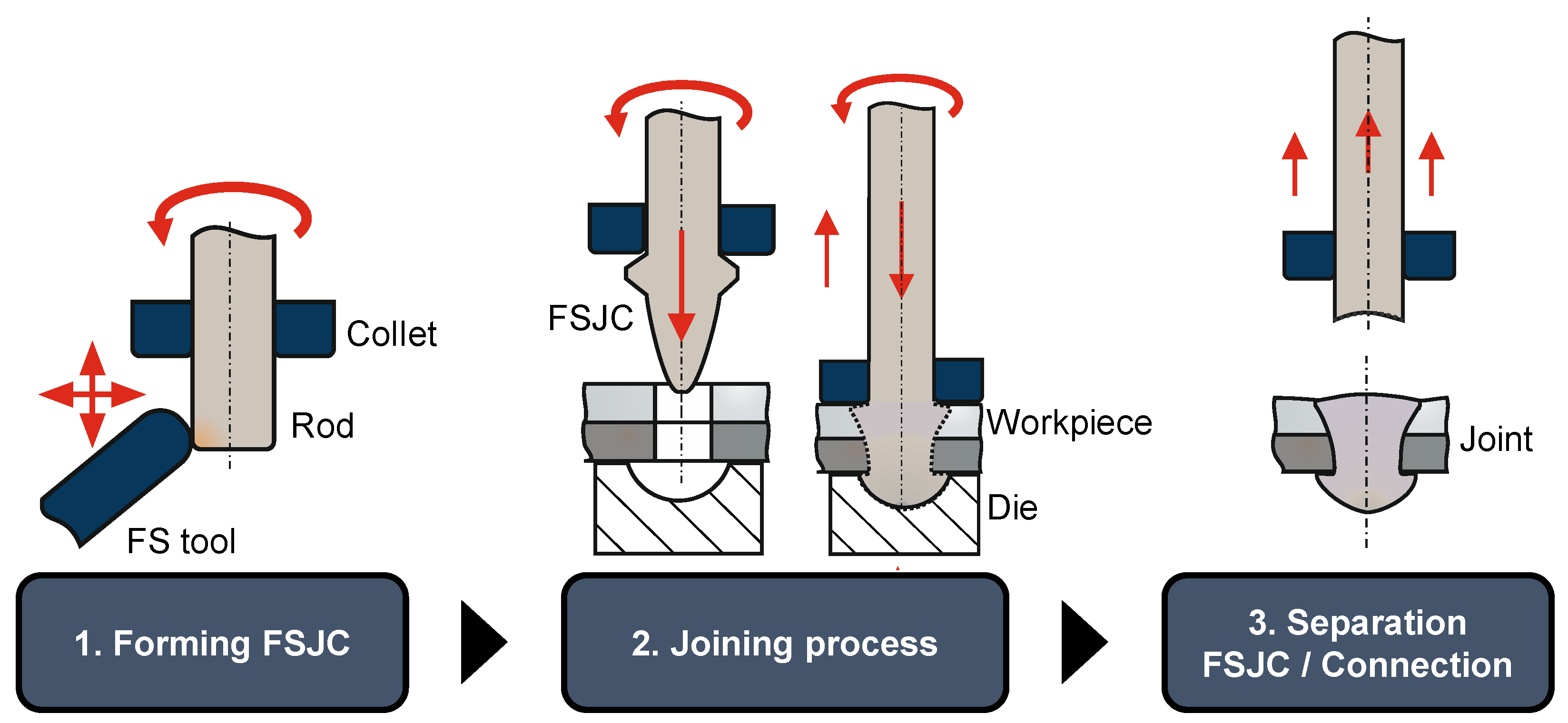
The adaptive joining process can be divided into three steps, which are illustrated in Figure 1: the thermo-mechanical kinematic shaping of the adaptive joining element; the subsequent joining process; and the final separation of the adaptive joining element from the initial material, e.g., by shearing. In the first step, the geometric shape, the mechanical properties, and the microstructure of the adaptive joining element are generated and adjusted by the use of friction spinning. Wischer et al. [3] thereby addressed the targeted setting of the microstructure.

Friction spinning is a thermo-mechanical process in which the workpiece is heated locally by means of friction and plastic deformation. The applied temperature reduces the yield stress of the material without exceeding its melting point. This increases formability and, at the same time, reduces the process forces required for forming. Friction spinning is also used in the actual joining process, which is shown as step 2 in Figure 2. The adaptive joining element is rotated and fed to the joint. It should be noted that a distinction can be made in the joining process between process strategies with pre-holed or non-pre-holed workpieces. Rostek et al. and Wischer et al. [1,2,3] went into more detail on the characteristics of these two strategies and included a detailed description of the adaptive joining technology, as well as a description of its adaptivity and the objects of investigation. In general, the selection of pre-holed or non-pre-holed workpieces depends on the material of the adaptive joining element. Aluminum alloys, for example, are not suitable for penetrating the workpieces and require an additional pre-holing operation to create a joint.

In the context of this paper, the adaptive joining technology with pre-holed workpieces is considered. As soon as the adaptive joining element comes into contact with the die, heat is generated as a result of friction. In addition to the (self-) induced friction heat, the shape generation of the joint is achieved by the axial feed stroke. Here, heat generation is additionally enhanced by plastic deformation and increases the formability of the workpiece. This has a positive effect on the formation of an interlock, which is significant for the mechanical strength of the joint. The forming process can also be adjusted in various ways according to the requirements of the joint, e.g., via the geometry of the die and the adaptive joining element, as well as via its mechanical properties, speed, and feed rate.

A comprehensive systematic investigation of this joining technology is the prerequisite for its realization. In conjunction with experimental investigations, such as those performed by Wiens et al. and Wischer et al. [2,3], numerical simulation using the finite element method (FEM) is to be used as a tool. With this modeling, numerical experiments can be performed to investigate, among other things, the material flow, the temperature distribution, the stresses, and the strains over the entire adaptive process. Numerical simulation can be used to gain a deeper understanding of the process. This allows parameters to be examined in isolation. In addition, it permits the analysis of process parameters that are difficult to access or even impossible to measure in the real process. One of the sub-goals of numerical simulation, for example, is to investigate the material flow and temperature distribution in the first and second steps of the adaptive joining process over the entire duration of the process. In addition, the experimental outlay can be reduced by means of simulative investigations. Hence, alternative die geometries and their influence on the material flow and the interlock formation are to be investigated by means of the FE model before being implemented experimentally. Therefore, the aim of this paper is to identify the requirements, boundary conditions, and approaches to FE modeling of this adaptive joining technology. It should be noted that this paper serves as a preparation for concrete research work and should be understood conceptually. Similar or related joining methods can be used for this purpose. Rostek et al. and Wischer et al. [1,3] related the adaptive joining technology to other and similar mechanical joining technologies. However, the two processes of friction drilling and friction stir welding are particularly suitable for comparative consideration with regard to simulative design.

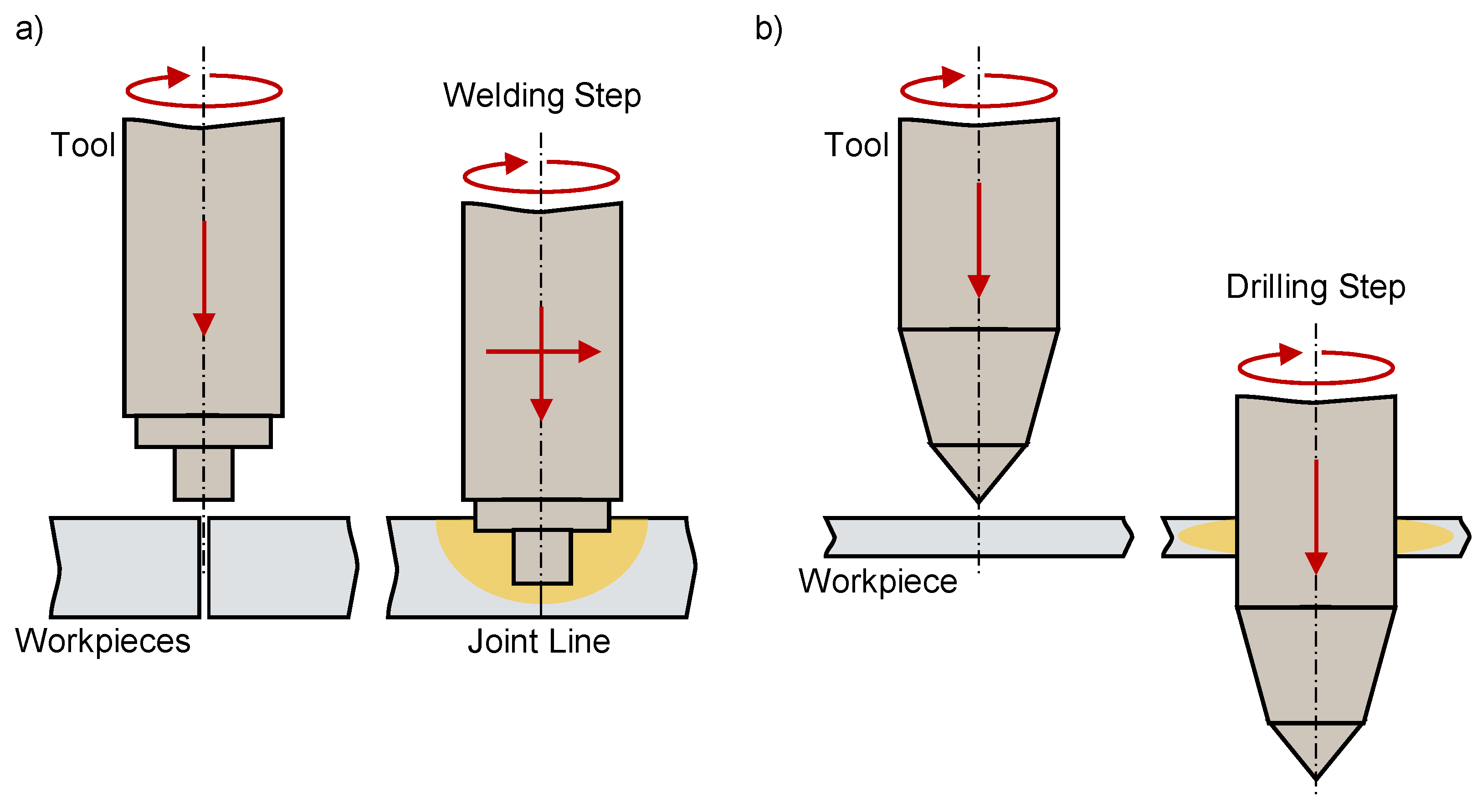
As with adaptive joining technology, both these technologies are solid state processes that use friction-induced heat to increase the formability of the material without exceeding its melting temperature. Figure 2 shows a schematic representation of both processes. Friction stir welding (FSW) is a joining, or rather a welding process. A rotating tool with a specially designed pin and shoulder is inserted into the abutting edges of the workpieces to be joined and moved along the joint line. Typically, the FSW process includes four steps: the plunging, dwelling, welding, and retracting steps [4,5,6,7,8,9,10,11]. In friction drilling (FD), which is also known as thermal drilling, thermo-mechanical drilling, forming drilling or flow drilling, a conical tool reams through a thin-walled workpiece to form a hole. In addition, the lateral extrusion of material typically results in the formation of a bushing, which is not shown in Figure 2 for the sake of simplicity [12,13,14,15,16,17,18]. Friction drilling corresponds largely to the adaptive joining process with non-pre-holed workpieces, since the workpieces must be drilled through prior to the actual joining process. However, the boundary conditions of FD, such as the kinematics and thermal boundary conditions, can also be transferred to other parts of the adaptive joining process.

When transferring the boundary conditions and modeling approaches of the two processes, their differences compared with the adaptive joining process must be considered. The tool geometry of both processes, for example, is usually less complex and less versatile, as was shown by Wiens et al. [2]. In addition, both friction stir welding and FD assume that the tool is a non-consumable tool, which neither wears nor deforms during the forming process. The adaptive joining element, by contrast, undergoes its main deformation both as it is being formed and during the joining process. In the adaptive joining process with non-pre-holed workpieces, the deformation of the workpieces must also be taken into account. The effect of these high degrees of deformation on numerical modeling and simulation will be discussed in more detail in the next section.

Another important difference between the processes under comparison is the rotational speeds used in each process. In FSW, rotational speeds of 800 to 1600 rpm are used [8,9,10]. Buffa et al. [7] also emphasized that there is currently a gap in knowledge regarding the modeling of high-speed FSW. As a possible reason for this, Buffa et al. [7] noted divergence problems due to mesh distortion intensified by the high rotational speeds. The rotational speeds used in FD are higher (800–4000 rpm) than the speeds for conventional FSW [13,14,15,16,17,18]. In the adaptive joining process, however, significantly higher rotational speeds of up to 12,000 rpm are used [3]. These high rotational speeds must be considered in numerical modeling, since they influence the strain rates and element distortions that occur and can also complicate contact detection.

The next section presents the detection of boundary conditions and the modeling approaches required for developing an FE process model of the adaptive joining process. Two reduced FE models are also presented for the forming of the adaptive joining element and for the joining process with a precut.

2. Simulative Requirements and Boundary Conditions

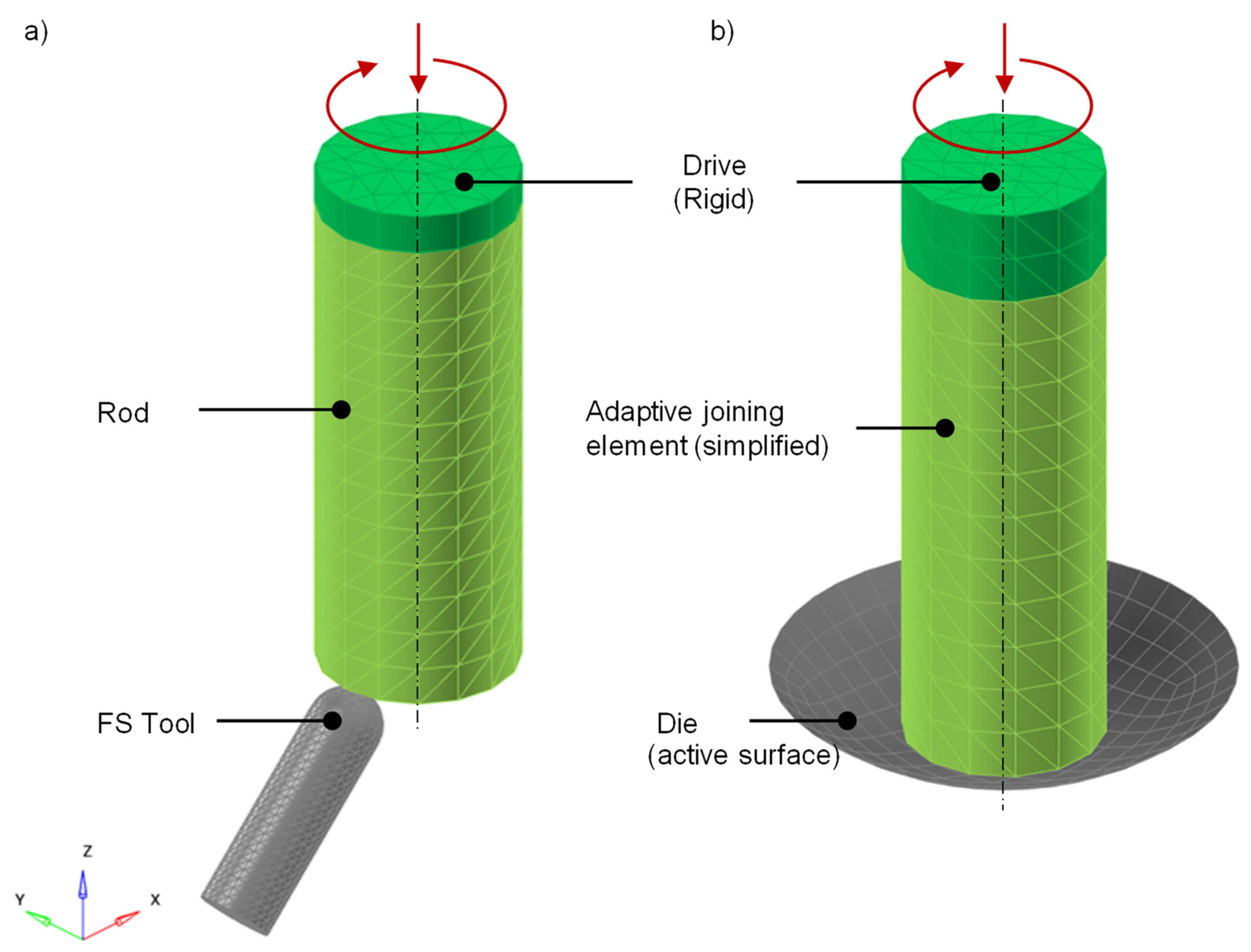
In order to be able to simulate all the process steps of the adaptive joining method, it is necessary to analyze them with regard to their requirements. For this purpose, a process comparison with FSW and FD is drawn up. In addition, initial modeling with the aid of two reduced models will be used to identify challenges and special characteristics associated with the numerical representation of the adaptive joining process. The structure of these models for forming the adaptive joining elements and the joining process with non-pre-holed workpieces is shown in Figure 3. Use is made of the FE program LS-DYNA (version R12.1, Livermore Software Technology, Livermore, CA, USA) within the scope of these investigations.

Simulative modeling of the adaptive joining process requires a thermo-mechanical coupling. For the mechanical solver, explicit time integration is chosen, due to the dynamic character of the process with comparatively high speeds of up to 12,000 rpm [3], and also due to the occurring nonlinearities such as those in the material, as well as through the complex contact situation and the high deformations. This is also the case for the two processes of FD and FSW. The thermal solver of LS-DYNA works with implicit time integration, which is why the convergence of the simulation must also be considered. Explicit time integration is a conditionally stable method. The critical time step ${\Delta \mathrm{t}}_{\mathrm{crit}}$, which must not be exceeded, is determined via the Courant-Friedrichs-Lewy-criterion, and can be expressed by the following equation:

$${\Delta \mathrm{t}}_{\mathrm{crit}}=\frac{2}{{\mathsf{\omega }}_{\max }}=\mathrm{l}\sqrt{\frac{\mathsf{\rho }}{\mathrm{E}} }=\frac{\mathrm{l}}{\mathrm{c}}$$

(1)

where ${\mathsf{\omega }}_{\max }$ is the maximum natural frequency of the system, $\mathrm{l}$ is the minimum characteristic length of all elements, $\mathsf{\rho }$ is the material density, $\mathrm{E}$ is the Young’s modulus, and c is the speed of sound in the material under consideration [19]. This criterion usually results in very small time steps into which a simulation must be divided. These small time steps contrast with the comparatively long process time of the adaptive joining process. The process times relevant for the simulation can be between 1 and 5 s. These long process times are accompanied by correspondingly high computational costs, which must be taken into account in the modeling. This problem also applies to FD, as described by Journaux et al. [16]. One approach to reducing the calculation costs is through the scaling methods of time and mass scaling. However, time scaling is not possible for the FE model of adaptive joining, due to the high strain rates that occur during the process and the strain rate-dependent material behavior. Mass scaling can be used, as was also the case in previous studies [10,13,14,18]. Since mass scaling artificially increases forces and temperatures, for example, it must be used with caution and thus constitutes a separate object of investigation.

For the simulation of the adaptive joining process, use is to be made of 3D modeling with LS-DYNA using the ton-mm-s-N unit system. The 3D FE model is necessary because the material deforms in a rotational direction during the forming of the adaptive joining element, as well as during the joining process. This also corresponds to the typical modeling of FSW and FD and was emphasized, inter alia, by Miller et al. [13].

The parts of the initial, reduced models were meshed comparatively coarsely, as can be seen in Figure 3. With this coarse spatial discretization, the process cannot be adequately represented due to the high degrees of deformation and the associated element distortions. The computational costs are, however, drastically reduced due to the greater minimum characteristic length of all the elements and the resulting reduction in the number of elements. Comparatively fast testing of different modeling approaches is thus possible, which will be discussed in this paper. The spatial discretization and the exact structure of the two FE models will also be discussed in more detail.

The model for forming adaptive joining elements consists of three parts: the drive, the rod, and the friction-spinning (FS) tool for forming the adaptive joining element. The drive is an auxiliary part, which is modeled as a rigid body and serves to apply the rotation and the feed. For its displacement boundary conditions (dbc), all degrees of freedom are therefore blocked, except for the translational degree of freedom in the z-direction and the rotational degree of freedom around the z-axis. The drive and rod are meshed by means of solid elements, with a mesh size ratio of 1.6 mm. The spatial discretization of the FS tool is significantly smaller, with a mesh size ratio of 0.4 mm, in order to be able to reproduce its geometric shape acceptably. In addition, the degrees of freedom of the FS tool with regard to the dbc are completely fixed. To form the adaptive joining element, the rod is fed at 250 mm/min at a speed of 8000 rpm for 1.224 s.

The joining process was modeled in a similar way. The FE model also consists of three parts: the drive, the adaptive joining element, and the die. The modeling of the pre-holed sheets was initially neglected. As before, the drive is an auxiliary body for generating the rotation and the feed. The geometry of the adaptive joining element is simplified as a cylinder. The drive and the adaptive joining element are meshed using solid elements with a mesh size ratio of 1.6 mm. To model the die, its effective area is meshed with square shell elements. This also reduces the computation time. However, for further investigations it is recommended that the die be meshed completely with solid elements to ensure that their thermal influence in respect of heat loss is adequately taken into account. With regard to the dbc of the die, all the degrees of freedom are completely locked. For initial investigations, the pre-heating phase is modeled. For this purpose, the adaptive joining element is fed at a rate of 20 mm/min and a speed of 20 rpm until it comes into contact with the die. After this, only a rotational movement at 2000 rpm takes place, which serves for heat input. Further approaches and boundary conditions for the reduced models will be discussed below.

It should be noted that the reduced FE models presented are only one approach to modeling the adaptive joining process. Another object of investigation in this respect is motion modeling by the rigid tools. In the case of the joining process (Figure 3b), the feed and rotation would be applied purely via the die. Experience has shown that implementing the motion completely via rigid bodies can have advantages in terms of stability, contact detection, and computation time. The extent to which these advantages apply to the modeling of the adaptive joining process, which modifications are appropriate, and the influences of this approach that need to be taken into account must be analyzed in future.

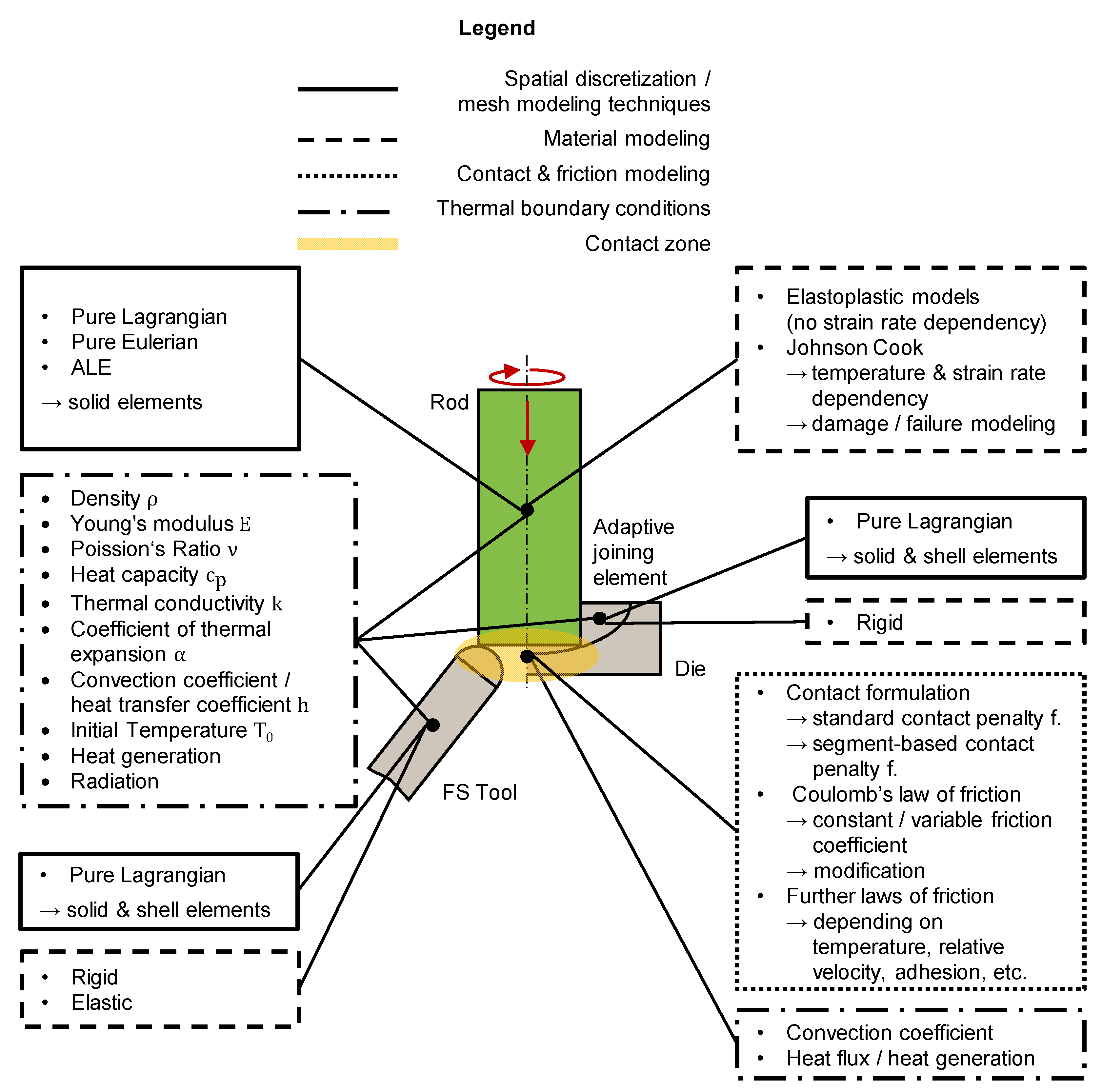
The detected requirements and boundary conditions are divided into the following subsections: spatial discretization and mesh modeling techniques, material modeling, contact and friction modeling, and thermal boundary conditions. An overview of these boundary conditions is shown in Figure 4. In addition, it should be noted that the investigations here were limited to numerical modeling, which realizes the spatial discretization by means of a mesh, in particular by the FEM. Other modeling approaches are also possible, however, which implement the spatial discretization in a different manner. One possibility is the discretization over particles by means of smoothed particle hydrodynamics (SPH), as used by Patil et al. and Journaux et al. [8,16].

2.1. Spatial Discretization and Mesh Modeling Techniques

In spatial discretization by means of a mesh, a distinction can be made between the selection of the element type and the mesh modeling technique.

In both FSW and FD, the tools are mostly meshed using solid elements as rigid bodies [8,10,15] or analytical rigid [13,17,18]. Shell elements for spatial discretization are used much less frequently [16,18]. However, meshing of the tool with solid elements is preferable to meshing with shell elements, since thermal boundary conditions, such as thermal conductivity and both heat transfer and heat loss over the entire tool, can be considered. As described above, solid elements were used to discretize all parts of the reduced FE models, except for the effective surface of the die, which was meshed with the help of shell elements. For future investigations, however, this process will also be modeled by solid elements.

With regard to the mesh modeling techniques, a distinction can be made between the following approaches: pure Lagrangian, pure Eulerian, and coupled approaches such as the Arbitrary Lagrangian Eulerian (ALE) approach.

In the Lagrangian approach, the mesh is firmly attached to the material. Thus, the mesh also deforms when the material undergoes deformation. However, the large deformations occurring in the adaptive joining process, as well as in FSW and FD, lead to high element distortions. These have a negative influence on the mesh quality, and hence on the quality of the result. In addition, strongly distorted elements can lead to instabilities in the implicit and the explicit solver, causing the calculation to be aborted. Therefore, pure Lagrangian approach is rarely used for modeling FSW and FD. If this approach is used, however, then it is used in combination with continuous remeshing, such as by adaptive remeshing [13,18], in order to minimize the element distortions.

In the Eulerian approach, the mesh serves as a background grid that does not deform as the material flows across it. The deformation in this case results when the material flows across an element node. For FSW and FD, the pure Eulerian approach is rarely used. In general, it is mostly used for fluid-mechanical mechanisms of the process and is limited to large deformations [11]. Meyghani et al. [9] used the pure Eulerian approach for areas of the semi-finished product that are not in the direct influence area (stirring zone) of the tool.

The ALE approach combines the Lagrangian approach with the Eulerian approach. Thus, element nodes do not have to precisely follow the material flow. They are repositioned if necessary to avoid strong element deformations. This allows the material to flow through the mesh, which is itself mobile. Thus, ALE is a well-suited method for mapping large deformations. However, a number of challenges or drawbacks must be borne in mind for its application. For example, the ALE approach increases the model size significantly, since two meshes are required and in most cases a large volume has to be meshed, which does not contain any matter [16]. This leads to a drastic increase in the number of elements, and an increase in the computational costs. However, modeling approaches do exist, which can alleviate this problem. For example, it is possible to move an initial mesh arbitrarily in space or to extend it if necessary. This avoids having to completely mesh the space in which the kinematics of a process takes place [19]. For the FE modeling of FSW and FD, previous studies [4,10,14,15] used the ALE approach. Meyghani et al. [9] combined the ALE approach for the area of influence of the tool on the semi-finished product, with a pure Eulerian mesh for all other areas of the semi-finished product. In addition, with regard to the adaptive joining process, the ALE approach is a promising methodology for spatial discretization. For the reduced models, however, the Lagrangian approach was initially chosen for gaining initial insights into further boundary conditions, such as contact modeling.

2.2. Material Modeling

When it comes to the material modeling of the adaptive joining process, the focus at this point should be on the deformable parts, i.e., the rod, the adaptive joining element, and the workpieces to be joined. It should be noted that during the joining process without precuts, it is necessary to consider the deformations of the adaptive joining element, as well as the workpiece. In contrast to FSW and FD, the actual tool, i.e., the adaptive joining element, cannot be assumed to be rigid. This, in turn, affects the contact modeling and the calculation times. In addition, the adaptive joining process places special demands on material modeling. This process should take into consideration the temperature dependence and the strain rate sensitivity of the material. In addition, there should be a possibility of damage modeling, which is particularly important for process modeling with non-pre-holed workpieces. These requirements correspond to those that FSW and FD place on material modeling, which is why a process comparison is also useful here. The rod or adaptive joining element is made of C45E, but it can also be manufactured from EN AW 6060 T6, which is particularly interesting for joining processes with pre-holed workpieces. A wide variety of materials can be used for the workpiece or workpieces to be joined. Joining processes with EN AW 6016 T6 and EN AW 6014 T4 have been investigated. In addition, studies of a wide variety of steel alloys and fiber-reinforced plastic composites are also planned. In both FSW and FD, deformable workpieces made of EN AW 6061 T6 have been frequently investigated [4,5,6,8,9,10,13,14,18]. Occasionally, FE models with steel workpieces have also been analyzed in FD [15,17].

For the material modeling of the workpieces for FSW and FD, different approaches have been used, which can be classified as elastoplastic material models and the Johnson-Cook model. The former were mainly used for material modeling of the workpieces in friction drilling.

Miller et al. [13] used an elastoplastic model and stated that this is only valid if the sensitivity of the material to high strain rate effects can be neglected. Miller et al. [18] also used a bilinear elastoplastic model that took kinematic hardening into account. A rate-insensitive and incompressible rigid perfect Mises plastic model was used by Kumar et al. for material modeling of the workpiece [15]. Journaux et al. [16] used an elastic viscoplastic model without kinetic hardening, which was implemented in LS-DYNA as *MAT_106/*MAT_VISCOPLASTIC_THERMAL. That application considered temperature dependent parameters, such as Young’s modulus, Poisson’s ratio, initial yield stress, and thermal expansion. LS-DYNA also offers the option of adding further temperature-dependent parameters by means of additionally defined thermal material models, e.g., *MAT_T01/*MAT_THERMAL_ISOTROPIC [20]. Miller et al. [13,18] linked their material modeling to a failure criterion in conjunction with an element deletion. Even though the elastoplastic models for modeling in FD can generate promising results, they are only suitable to a limited extent for modeling in the adaptive joining process. This is due to the fact that the elastoplastic approaches do not take the strain rate effects of the material into account, which should not be neglected due to the high rotational speeds that occur.

A material model that takes into account both strain- and temperature-sensitive plasticity is the Johnson-Cook model. Moreover, this model remains valid at low strain rates and even into the quasi-static range. In LS-DYNA it is implemented as *MAT_015/*MAT_JOHNSON_COOK, as well as *MAT_224/*MAT_TABULATED_JOHNSON_COOK. The latter represents an elasto-viscoplastic material behavior with the possibility of considering arbitrary stress-strain curves for arbitrary strain-rate dependencies. In addition, this material modeling offers the option of activating damage or failure modeling and erosion with element deletion [20]. The Johnson-Cook model was frequently used for FSW, as well as for FD [8,9,10,11,12,14]. In addition, Dehghan et al. [14] considered the Johnson-Cook failure model with an element deletion. Since the requirements of the adaptive joining process for material modeling are fulfilled by the Johnson-Cook model, it was selected for the rod as well as for the adaptive joining element of the reduced models.

The material modeling of the non-deformable tool was realized as a rigid body for FSW and FD [4,7,8,9,10,12,13,15,16,17,18]. For the adaptive joining process, this applies to the FS tool, as well as to the die. First investigations showed that the FS tool can also be defined as ideally elastic with *MAT_001/*MAT_ELASTIC in order to counteract an unrealistic generation of contact forces. This consideration will be discussed in more detail in the next subsection.

2.3. Contact and Friction Modeling

With regard to contact modeling, two main subjects of investigation can be identified: contact detection and friction modeling.

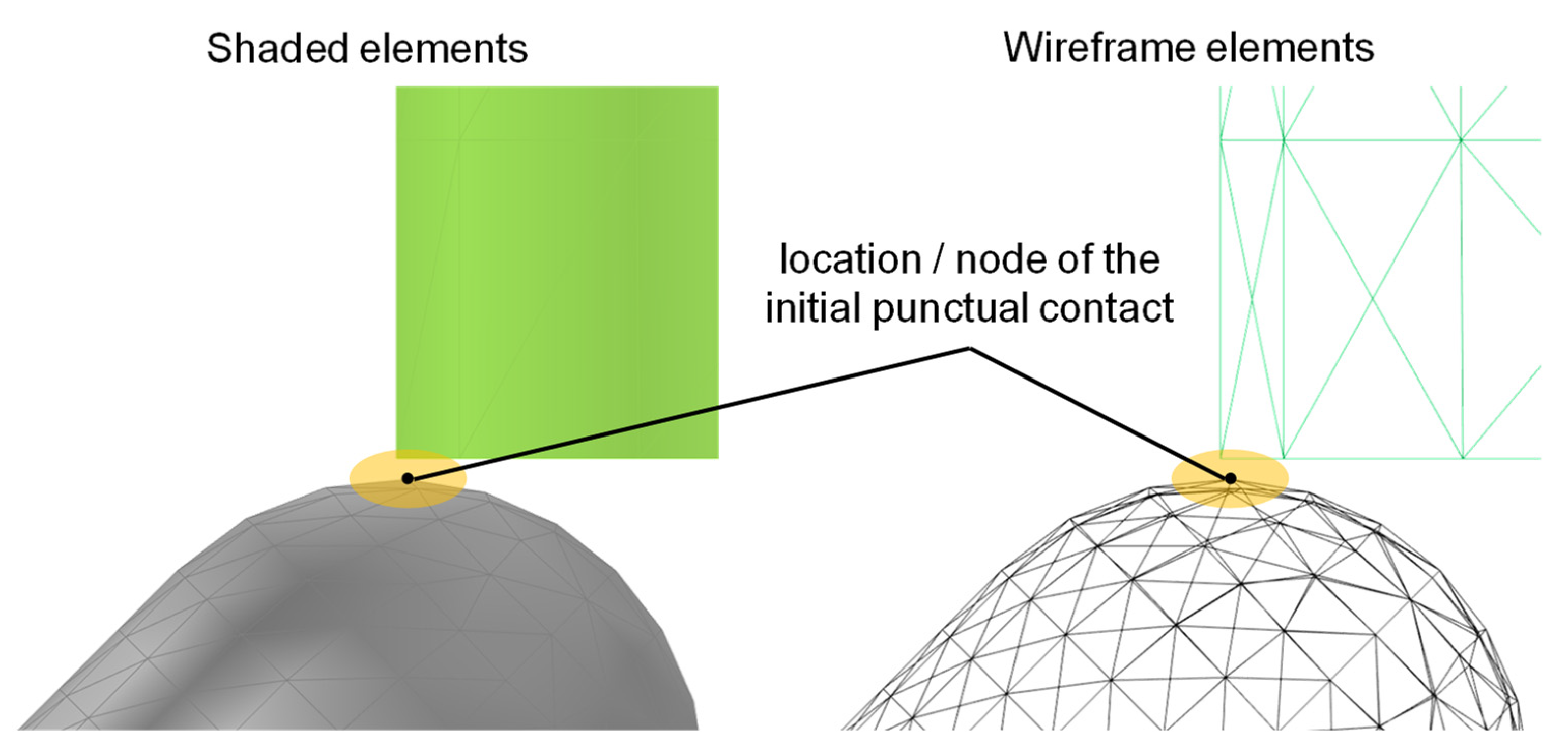
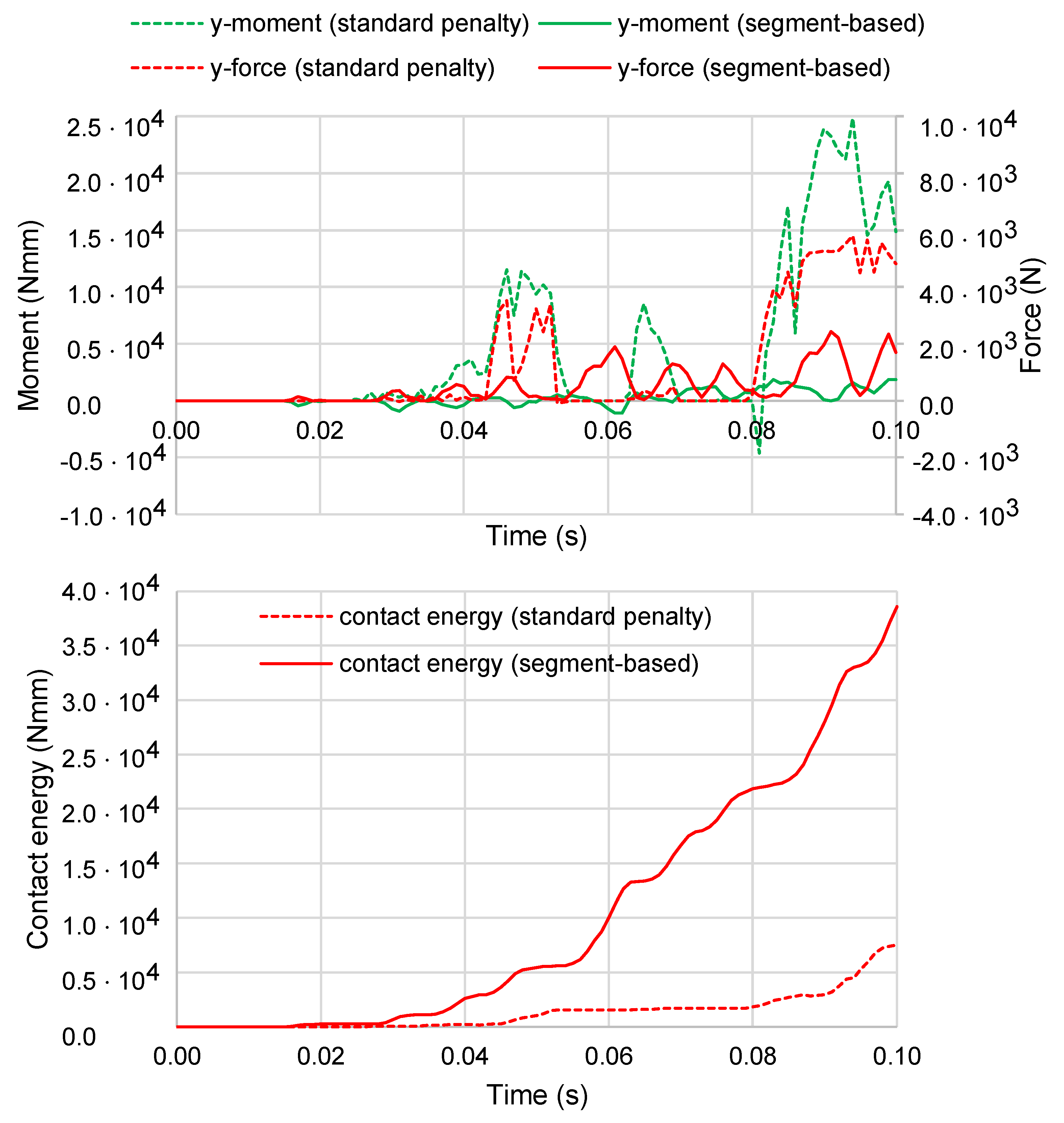
The problem of contact detection is particularly evident in the reduced model of adaptive joining element forming. Initially, this was modeled using the *CONTACT_AUTOMATIC_SURFACE_TO_SURFACE contact with the standard contact penalty formulation. In addition, friction was initially neglected in order to study the contact detection problem independently. Figure 5 shows the contact situation between the FS tool and the rod. The discretization of the tool with solid elements initially results in a punctual contact at the time of 0.024 s. In conjunction with the comparatively high rotational speed, this causes unrealistically high contact forces and moments, which are particularly pronounced in the y-direction.

Figure 6 shows these curves for the contact force and the contact moment in the y-direction for 0.1 s of the process. This leads to a deflection of the rod, the cause of which is purely numerical and cannot be observed experimentally. In addition, the nodes of the rod “stick” to the FS tool. The nodes get caught and remain stuck for a short time instead of gliding smoothly. This is also visible from the contact energies in the form of sudden jumps, which are an indication of numerical instabilities of the contact. The course of the contact energies is also shown in Figure 6. It should be borne in mind that with the standard contact penalty formulation, the deflection of the rod causes a loss of contact between the tool and the rod at approx. 0.054 s. Therefore, only comparatively low contact energies are generated.

To overcome the problem of contact detection, the segment-based contact penalty formulation was investigated, which can be activated in the contact-card via SOFT = 2. This formulation checks for segment vs. segment penetration, rather than node vs. segment penetration [19]. Furthermore, additional contact options can be activated. Using SBOPT = 5, warped element checking and a sliding option were activated. The latter is recommended for preventing segments from incorrectly catching nodes on a sliding surface [19]. Figure 6 shows the contact force and the contact moment in the y-direction, as well as the contact energy generated with this contact formulation. Here, it is clear that both the force and the moment are significantly lower than the standard contact penalty formulation. In addition, there is no deflection of the rod, and hence no loss of contact. Therefore, the contact energies are also significantly higher when using the segment-based contact formulation. Compared to the standard penalty contact formulation, the contact energy curve is also smoother. However, there are still jumps in the contact energy curve.

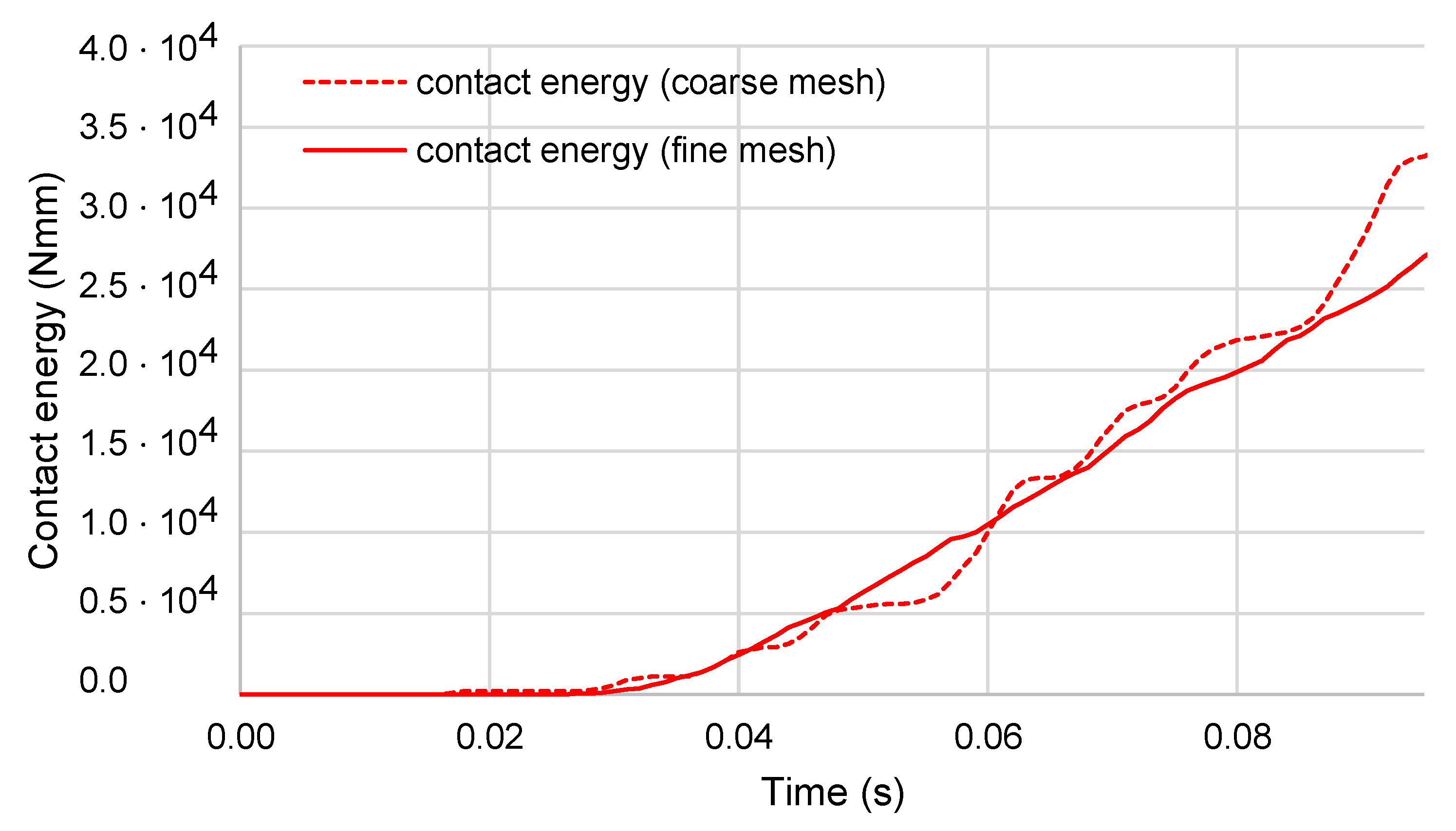
One reason for this could be the coarse meshing of the rod. The rod was thus re-meshed with a mesh size ratio of 0.4 mm. Figure 7 shows the generated contact energies in comparison to the energies generated with the coarse spatial discretization. Here, it is evident that the progression is significantly smoother. Even with the finer meshing, however, critical element distortions occur with a significantly increased computation time, which is more than seventy times the computation time for the coarsely meshed model. From this it can be concluded that further investigations of contact detection, in conjunction with alternative approaches for spatial discretization, are indispensable.

In addition to the contact formulation, the material modeling of the FS tool constitutes another option for reducing the forces caused by the punctual contact, which act on the rod and lead to its deflection. For this purpose, the FS tool was defined as an elastic body, as described in Section 2.2. This is a more realistic assumption than that of a rigid body. Experimental investigations have shown that the tool undergoes elastic deformation counter to the direction of feed and rotation during forming, but no plastic deformation. The elastic tool definition was investigated in conjunction with the segment-based contact penalty formulation and the coarse meshing of the rod. It was found that this definition has a positive effect on contact detection. However, as a consequence of the coarse discretization, instabilities of the contact energy occur, and a slight deflection of the rod can also be observed. In addition, the computational costs increase more than sevenfold. With a finer discretization, this increase can be expected to rise significantly due to the enhanced element number. Despite this challenge, elastic tool definition is an important area of investigation that should be pursued.

Friction modeling is also an important subject of investigation. The process comparison with FSW and FD shows that Coulomb’s law of friction is most commonly used for FE modeling. Previous studies [5,6,8,12,13,15,18] used the law of friction with constant friction coefficients. Modeling with variable coefficients of friction is also possible. Xu et al. and Meyghani et al. [4,11] used a modified Coulomb’s law of friction, where the tangential stress is limited to a constant value and cannot theoretically increase to infinity. Coulomb’s law of friction is often used, but it is also often stated that this simple friction model is not suitable for the complicated friction phenomenon, as was stated, e.g., by Miller et al. [13]. Coulomb’s law of friction also forms the basis of friction modeling in LS-DYNA. Here, in addition to specifying a static and dynamic friction coefficient, the friction coefficient ${\mathsf{\mu }}_{\mathrm{c}}$ can also be calculated using the following equation:

$${\mathsf{\mu }}_{\mathrm{c}}=\mathrm{FD}+\left(\mathrm{FS} - \mathrm{FD}\right){\mathrm{e}}^{-\mathrm{DC}\left|{\mathrm{v}}_{\mathrm{rel}}\right|}$$

(2)

where $\mathrm{FD}$ is the dynamic coefficient of friction, $\mathrm{FS}$ is the static coefficient of friction, $\mathrm{DC}$ is the exponential decay coefficient, and ${\mathrm{v}}_{\mathrm{rel}}$ is the relative velocity [19]. It is also possible to specify the coefficient of friction as a function of pressure and relative velocity.

Coulomb’s law of friction is not sufficient for modeling the friction phenomena occurring in the adaptive joining process. Since, among other things, the shear yield stress is exceeded here, the process is outside the validity range of Coulomb’s law of friction. Accordingly, another important research subject will be the identification of additional friction laws, which take into account, for example, dependencies on temperature, relative velocity, or the adhesion of the material to the FS tool. These can then be implemented in LS-DYNA via subroutines and examined for their suitability for modeling the adaptive joining process.

2.4. Thermal Boundary Conditions

When it comes to the thermal boundary conditions, the calculation of the heat generation, as well as the thermal characteristic values and parameters, is of particular importance. The governing equation for the thermal model is given by

$$\mathsf{\rho }\cdot {\mathrm{c}}_{\mathrm{p}}\frac{\mathsf{\delta }\mathrm{T}}{\mathsf{\delta }\mathrm{t}}=\mathrm{k}\left[\frac{{\mathsf{\delta }}^2\mathrm{T}}{{\mathsf{\delta }\mathrm{x}}^2}+\frac{{\mathsf{\delta }}^2\mathrm{T}}{{\mathsf{\delta }\mathrm{y}}^2}+\frac{{\mathsf{\delta }}^2\mathrm{T}}{{\mathsf{\delta }\mathrm{z}}^2}\right]+\mathrm{G}$$

(3)

where $\mathsf{\rho }$ is the density, ${\mathrm{c}}_{\mathrm{p}}$ is the specific heat, $\mathrm{T}$ is the temperature, $\mathrm{t}$ is time, $\mathrm{k}$ is the thermal conductivity, $\mathrm{x}, \mathrm{y}, \mathrm{z}$ are the spatial coordinates, and $\mathrm{G}$ is the heat generation rate [13]. This results from the following equation:

$$\mathrm{G}=\dot{{ \mathrm{q}}_{\mathrm{f}}}+\dot{{ \mathrm{q}}_{\mathrm{p}}}$$

(4)

where $\dot{{ \mathrm{q}}_{\mathrm{f}}}$ is the frictional heat generation and $\dot{{ \mathrm{q}}_{\mathrm{p}}}$ the heat generation rate due to irreversible plastic deformation [13]. For the frictional heat generation rate, taking into account Coulomb’s law of friction and a rotating cylindrical tool, the following is obtained:

$$\dot{{\mathrm{q}}_{\mathrm{f}}}=2\mathrm{\pi }·\mathrm{r}·\mathrm{n}·\mathsf{\mu }·{\mathrm{F}}_{\mathrm{n}}$$

(5)

where $\mathrm{r}$ is the tool radius, $\mathrm{n}$ is the rotational speed, and ${\mathrm{F}}_{\mathrm{n}}$ is the normal force. The heating rate due to plastic deformation is shown by the following equation:

$$\dot{{\mathrm{q}}_{\mathrm{p}}}=\mathsf{\eta }\mathsf{·}\mathsf{\sigma }\mathsf{·}{\dot{\mathsf{\epsilon }}}^{\mathrm{pl}}$$

(6)

where $\mathsf{\eta }$ is the inelastic heat fraction, $\mathsf{\sigma }$ is the effective stress, and ${\dot{\mathsf{\epsilon }}}^{\mathrm{pl}}$ is the plastic strain rate [13]. Since frictional heat generation is based on Coulomb’s law of friction, whether an alternative law of friction is more suitable for heat generation in the adaptive joining process can also be investigated.

For thermo-mechanical coupling, the following thermal characteristic values and parameters must be considered:

• Density $\mathsf{\rho }$
• Young’s modulus E
• Poisson’s ratio ν
• Heat capacity c_p
• Thermal conductivity k
• Coefficient of thermal expansion α
• Convection coefficient/heat transfer coefficient h

These characteristic values can be specified both as temperature-independent constants and as temperature-dependent values, provided that the temperature modeling selected allows this. In the modeling of FSW and FD, constant, temperature-independent characteristic values are occasionally assumed, as was done by Miller et al. [17]. However, temperature-dependent characteristic values positively influence the accuracy of the model, so it is recommended that use be made of these values [10]. Previous studies [13,16,18] used temperature-dependent characteristic values for their modeling. Convection is mostly assumed as a constant value; assumptions can be made in this respect. For example, free convection was assumed by Miller et al. [17]; Miller et al. and Vijayabaskar et al. [13,18] took into account the convection on the upper surface of the workpiece, and for Dehghan et al. [14] the convection on the lower surface of the workpiece was also considered. Kumar et al. [15] assigned a constant convection coefficient to all surfaces of the workpiece and the tool.

The tool’s thermal degrees of freedom are often neglected or not fully considered in the modeling of FSW and FD. The latter is especially the case if the tool has been discretized with shell elements ([16,18]). Meyghani et al. [9] did not consider the thermal degrees of freedom of the tool at all. This reduction cannot be applied in the modeling the adaptive joining process, since the thermal degrees of freedom play a decisive role in heat generation and hence for the material flow of the process steps.

In addition to the characteristic values, further thermal boundary conditions must be taken into account. For example, the thermal FE analysis always requires the definition of the initial/ambient temperature ${\mathrm{T}}_0$. This is usually assumed to be between 20 and 25 °C [11,13,14,15,18]. Heat generation can also be modeled using different approaches. This can be applied artificially in the form of a heat flux [4,17]. However, it is also possible to consider the heat generation due to friction and plastic deformation, as was done in previous studies [5,8,13,18]. Song et al. and Dehghan et al. [6,14] only accounted for the heat generation as a result of friction and neglected the share of plastic deformation in this. Due to the high degrees of deformation during the adaptive joining process, such a simplification should not be made. Another important subject of investigation is the consideration of radiation and the associated heat loss. This is often neglected in FSW and FD modeling. For example, Kumar et al. [15] stated that the heat losses due to radiation were small and therefore radiation could be neglected in the FE modeling. However, Meyghani et al. stated that consideration of radiation is recommended for large area components, such as the top and bottom of the sheets in FSW. This recommendation can be applied to the modeling of the sheets in the adaptive joining process. The role the radiation plays in shaping the adaptive joining element should also be investigated, together with whether the radiation should be included here, as well as the die, in the joining process.

In summary, the thermal boundary conditions play an important role for the FE modeling of the adaptive joining process. The analysis of these conditions in connection with the law of friction and with the contact modeling constitutes a central object of investigation.

3. Conclusions and Outlook for Future Investigations

This paper covered the identification of requirements and boundary conditions for the numerical modeling of the adaptive joining process. It serves as a conceptual preparation for future research. For this purpose, the process was compared with the two related processes of FSW and FD. The comparison included highlighting the differences between these processes and the adaptive joining process, especially concerning the tool, its deformation during the joining process, and the rotational speeds that occur in the respective process, which are significantly lower than those for the adaptive joining process. The process comparison was also used to analyze the boundary conditions, which were divided into the spatial discretization and mesh modeling techniques, the material modeling, the contact and friction modeling, and the thermal boundary conditions. Two reduced FE models of the forming of the adaptive joining element and of the joining process were also described and used for initial investigations of these boundary conditions.

In terms of the spatial discretization, the Lagrangian approach is insufficient to represent the deformations that occur. Instead, the ALE approach should be used. Furthermore, spatial discretization methods that are not based on the generation of a mesh should be investigated. Examples are particle-based methods such as SPH or the element-free Galerkin method. With respect to material modeling, the Johnson-Cook model is a promising model due to its consideration of temperature and the behavior of strain-rate-dependent material. Contact detection was also an important subject of investigation. The standard contact penalty formulation is not sufficient for contact detection in the adaptive joining process, and the segment-based contact formulation in combination with an alternative spatial discretization approach should be investigated instead. Friction modeling was also of particular importance in conjunction with the contact. The frequently used Coulomb’s law of friction is not sufficient to represent the complex friction phenomena of the adaptive joining process, and the identification and investigation of further friction laws is required. When it comes to the thermal boundary conditions, the use of temperature-dependent characteristic values is advantageous. Furthermore, the thermal degrees of freedom of the workpieces and of the tools should be taken into account. In addition to the investigation of heat generation, an investigation of the influence of radiation on the process steps of the adaptive joining process is indispensable.

Further analysis of the FE modeling of the adaptive joining process requires the development, verification, and validation of more complex process models based on the identified requirements and constraints described in this paper. For this purpose, further research on FE modeling of FSW and FD is recommended. An extension of this research to other related processes, such as friction welding, would also be possible.