Optimization-Based Data-Enabled Modeling Technique for HVAC Systems Components


1
Department of Civil and Architectural Engineering and Construction Management, University of Cincinnati, Cincinnati, OH 45221, USA
2
Department of Architectural Engineering, Gachon University, Seongnam-si 1342, Korea
*
Author to whom correspondence should be addressed.
Buildings 2020, 10(9), 163; https://0-doi-org.brum.beds.ac.uk/10.3390/buildings10090163
Submission received: 31 July 2020
/
Revised: 10 September 2020
/
Accepted: 11 September 2020
/
Published: 13 September 2020
(This article belongs to the Special Issue Modeling, Analysis, Optimization and Control of HVAC Systems in Buildings)
Abstract
:Most of the energy consumed by the residential and commercial buildings in the U.S. is dedicated to space cooling and heating systems, according to the U.S. Energy Information Administration. Therefore, the need for better operation mechanisms of those existing systems become more crucial. The most vital factor for that is the need for accurate models that can accurately predict the system component performance. Therefore, this paper’s primary goal is to develop a new accurate data-driven modeling and optimization technique that can accurately predict the performance of the selected system components. Several data-enabled modeling techniques such as artificial neural networks (ANN), support vector machine (SVM), and aggregated bootstrapping (BSA) are investigated, and model improvements through model structure optimization proposed. The optimization algorithm will determine the optimal model structures and automate the process of the parametric study. The optimization problem is solved using a genetic algorithm (GA) to reduce the error between the simulated and actual data for the testing period. The models predicted the performance of the chilled water variable air volume (VAV) system’s main components of cooling coil and fan power as a function of multiple inputs. Additionally, the packaged DX system compressor modeled, and the compressor power was predicted. The testing results held a low coefficient of variation (CV%) values of 1.22% for the cooling coil, and for the fan model, it was found to be 9.04%. The testing results showed that the proposed modeling and optimization technique could accurately predict the system components’ performance.
1. Introduction
In 2017, about 38 quadrillion British thermal units of the total U.S. energy consumption was consumed by the residential and commercial sectors, according to the U.S. Energy Information Administration. Where it was found that in 2012, the space heating consumes most of the overall energy use in commercial buildings [1]. Moreover, the advanced global revenue will grow from $7.0 billion in 2014 to $12.7 billion in 2023. In addition to the electricity prices that are rapidly increasing and the increasing cost of operating the heating ventilation and air condition (HVAC) systems in the buildings, the buildings are responsible for 44.6% of the total CO2 emissions, which is the most significant portion compared to 34.3% for transportation and 21.1% for the industry sector. Thus, the need for better operation mechanism of those existing systems become more crucial [2,3]. HVAC systems are heating, ventilation, and air conditioning systems that are responsible for heating and cooling the space as well as ventilation to maintain the inhabitant comfort levels. HVAC systems are complex nonlinear systems that have different variables as the parameters of those systems. Many studies have been done to understand those systems fully as well as reducing the energy consumed by them [4]. Even though the HVAC systems operate using the same thermodynamics principles, they still have different applications depending on the building type.
Chilled water HVAC systems are one of the most popular HVAC systems. They are sized for numerous building types where careful consideration must be taken in the design process [5,6]. On the other hand, packaged DX systems (packaged direct expansion systems) are a popular system that is mostly used in commercial and office buildings throughout the United States. They are known for their reliability and compact design. Additionally, they are accountable for 54% of the cooling energy for commercial buildings [7,8]. The DX system and chilled water system models are derived from a combination of physical models of the components. The components are compressor, cooling coil, condenser, heat pipes, fans, and outdoor air mixing chambers, etc. [9].
HVAC systems are a complex nonlinear structure that consists of heat and mass transfer equipment. They also consist of sensors, controllers that control several variables of the system. Thus, to predict the energy consumed by those systems, there is a need to measure and model the individual components of the system from either measured data or from knowledge previous physical laws and methods [10]. Models can be divided into two: forward models and data-driven models. Forward models are based on engineering principles and usually required detailed physical information. The use of physical models in real system operations requires detailed physical information that may not always be available. It requires elevated time to complete the calculations that may exceed the optimization period. Therefore, physical models are rarely used for real-time operations. On the other hand, the data-based models do not need any information on the system, and they can simply be used for such real-time applications. As real-time performance data are available in most modern building automation systems BASs, data-enabled model-based techniques may be the most effective way to achieve optimally secured and demand flexible building energy system operations [11,12].
An adequately identified model can provide accurate or close to accurate results and, at the same time, may require minimum calculations time [13]. Therefore, creating an accurate model by accurately identifying their parameters became crucial.
While HVAC systems have certain features like nonlinearity, time-dependent, time-varying system dynamics, insufficient data, complex interactions between the components, and limited supervisory controls, thus modeling the HVAC systems is a very characteristic and challenging process [14]. Therefore, while developing an HVAC system and component model, close attention should be given to deciding on the accurate model structure, model parameters, and constraints [15]. So that the final selected model can accurately deal with disturbance, constraints, and uncertainties, to control the time-varying applications and time delays, and to handle a broad range of operating conditions.
Numerous data-driven models and techniques that are designed to predict the performance of the HVAC component and attempt to optimize the performance of it are now found [16]. Optimization is a process in mathematics that is used to maximize and minimize a specific function. One of the most popular optimization methods is the genetic algorithm (GA). GA is an optimization technique that is based on the theory of natural selection. GA is implemented in the process of design to minimize the cost and maximize the efficiency [17].
However, there have been some shortcomings that are associated with previous studies. Some of those shortcomings are that the models were developed on assumptions and metrics that needed to be justified, and some of the modeling techniques used, need to be further discussed to justify the selection of each modeling technique and not another. Moreover, some of those models are not flexible enough to be used in other HVAC systems.
As previously stated, to accurately predict the energy consumption of the HVAC system. Two-level of optimization need to be integrated. The first level is the component model optimization level. At the same time, the second level is a system performance optimization level. This paper’s primary goal is to develop a new accurate data-driven modeling and optimization technique that can accurately predict the performance of the selected system components (first level of optimization). The proposed approach can be used to predict the performance of the components of the typical chilled water system and packaged DX systems.
Research Background
The problems surrounding building energy performance arise from the infinite architectural and mechanical building designs and multiple energy analysis methods and tools available. Energy efficiency is achieved through adequately functioning equipment and control systems. Therefore, implementing a high-efficiency HVAC plant is a must to guarantee the low running costs of the desired facility. Thus, a study was conducted on a historical building (the San Martino Castle in Parella), which discussed the criteria that can drive the process of upgrading the exciting HVAC plant as follows, giving new life to the environment, achieving adequate IAQ levels, respecting the existing structure, minimizing terminals and distribution systems, and installing the efficient system that will reduce the emissions and cost [18].
Whereas, in exciting systems, problems associated with building controls and operation are the primary causes of inefficient energy usage. Therefore, modeling and simulation of building system performance has a significant impact on energy savings [19]. One drawback of energy-saving predictions that are being used now, is using physical-based estimated data. Estimated data that are based on the physical models and equations, do not give the right estimation for building performance because they do not account for many factors like building occupants. Therefore, using actual performance data or simulation data for energy savings approaches will give a more accurate result, since they account for factors such as occupant behavior, operational inefficiencies, and interactive effects that are difficult or costly to account for in building energy models [20]. Where a study compared the design stage estimated data vs. the actual performance in the building using NBI’s (New Buildings Institute) database of LEED (Leadership in Energy and Environmental Design) certified buildings. The study found that measured EUIs for 50% of the buildings deviated by about 25% from the projected performance, with 30% significantly better and 25% significantly worse [21]. Since most of the recent buildings HVAC systems controlled with a BAS system not only to collect data but to ensure occupant comfort [22]. Therefore, there has been an increase in the number of actual building performance data. The recent availability of more data to use has smoothened the process of developing data-driven algorithms that can be used for more accurate and flexible energy savings predictions, and they represent an excellent opportunity for building commissioning [23]. Data-driven models and machine learning are used in many aspects of modern society [24]. Data-driven models that are based on real systems data are proven to be helpful tools in understanding the performance of HVAC systems and explain the relationship of the system components [15,25]. Moreover, those data-based modeling techniques are aimed towards improving the indoor air quality of the building (IAQ) as it is causing concern in the overall human health and comfort levels [26,27]. Air handling units (AHU) are nonlinear systems, and it makes it hard to maintain thermal comfort. A data acquisition system using ANN developed to control the performance of AHU [28]. Moreover, a study has been conducted to a baseline case of one zone using ANN. The inputs were weather, occupancy, and indoor temperature. The goal of the study was to minimize energy consumption. A genetic algorithm engine optimized the model. The research has shown a 25% reduction in energy consumption compared to the baseline heating strategy [29].
However, one of the shortcomings of the previous studies is that very few models have used real performance data that are collected in a long period [30]. Most of the researches that we found has trained their models using simulation data or a limited set of data collected in a short period [31]. Which more likely effected the accuracy of the predictions. For example, a study conducted by [32] to model the building systems using MATLAB TM. They considered the building as a thermal network; also, they used one season of data. Therefore, the model can be considered an incomplete model because it was covering only the winter season, so only the heating system was evaluated. Moreover, developing models using a limited range of data is not accurate for predicting the indoor temperature and relative humidity, unlike other studies that developed models using a short period. Other studies have made their first objective to collect data on a more extended period, not less than a year, to get accurate results [33]. A study conducted by [34] developed models using an extended period (nine months). The study has found that no model can predict the indoor temperature and humidity levels. This conclusion is contradicting with [35], who used a shorter period. The results have changed when expanding the period of data collection, indicating that more extended periods of data observation and collection will result in a more accurate energy prediction.
An adequately identified model can provide accurate energy prediction. Therefore, creating an accurate model by accurately identifying their parameters became crucial. Parameters identification that is influenced by input data, excitation signals, and model structure is an essential factor in system identification accuracy and efficiency [36]. Even though parametric testing methods are crucial to determine the system order, there is still a lack of a methodical approach for the model structure selection, order determination, and parameter identification [37]. Most of the existing studies nowadays are using the trial and error approach to decide on the model structure, order, and parameters [13]. Thus, researchers have studied several ways of optimizing the HVAC systems component and performance in both conventional methods and data-driven methods. References [38,39] have discussed energy savings conventional control strategies, and optimization for variable air volume (VAV) systems. In addition to the traditional methods of optimization, there have been data-driven approaches to optimize the HVAC systems in one level of optimization as well as integrated multiple levels and algorithms of optimizations [40]. Like, an integrated optimization technique proposed that can predict the supply air temperature and static duct pressure of the air handling unit. The optimization technique will integrate four component models of a chiller, pump, fan, and a reheating device using MLP (multiple-liner perceptron) methods. The results have demonstrated an energy saving of 7% of the total consumption of the unit [16]. Additionally, a study conducted by [41] has demonstrated an optimization algorithm for office buildings, which considered the comfort ranges of temperature, humidity, and thermal adaptation capability. The results of the study have proven that the proposed optimization technique can efficiently maintain occupant comfort levels while maintaining low energy used compared to conventional buildings.
Moreover, genetic algorithm (GA) was proven by previous studies to be an efficient tool for optimizing the HVAC modeling process when implemented on a whole system level and component level [42]. A study was conducted by [43] to develop an HVAC system optimization control strategy involving a fan coil unit temperature control for energy conservation in chilled water systems. The genetic algorithm was one of the tools selected to optimize system performance. The study conducted a field experiment, and the results have demonstrated that the proposed strategy has resulted in a 39.71% energy conservation when compared against another system operating at a full load. However, studies have shown that the computational intelligence approaches have been developed on the emphasis of optimizing energy consumption first, followed by the optimization of thermal comfort, then indoor air quality, and occupant preferences [44].
Therefore, in this research, a data-driven optimization technique was proposed to optimize the performance of the HVAC systems component (component model optimization) as part of optimizing the whole system performance (system performance optimization). The study has addressed most of the shortcomings of previous studies, where the models where tested and trained on real building performance data. The data were collected for a more extended period (one year). A comparison between multiple available modeling tools was conducted to decide on the best modeling technique that will be later used. The selected modeling tool was tested and trained to choose the best model structure. A model level optimization technique using GA was implemented to automate the process of selecting the best model structure.
2. Proposed Modeling Strategy
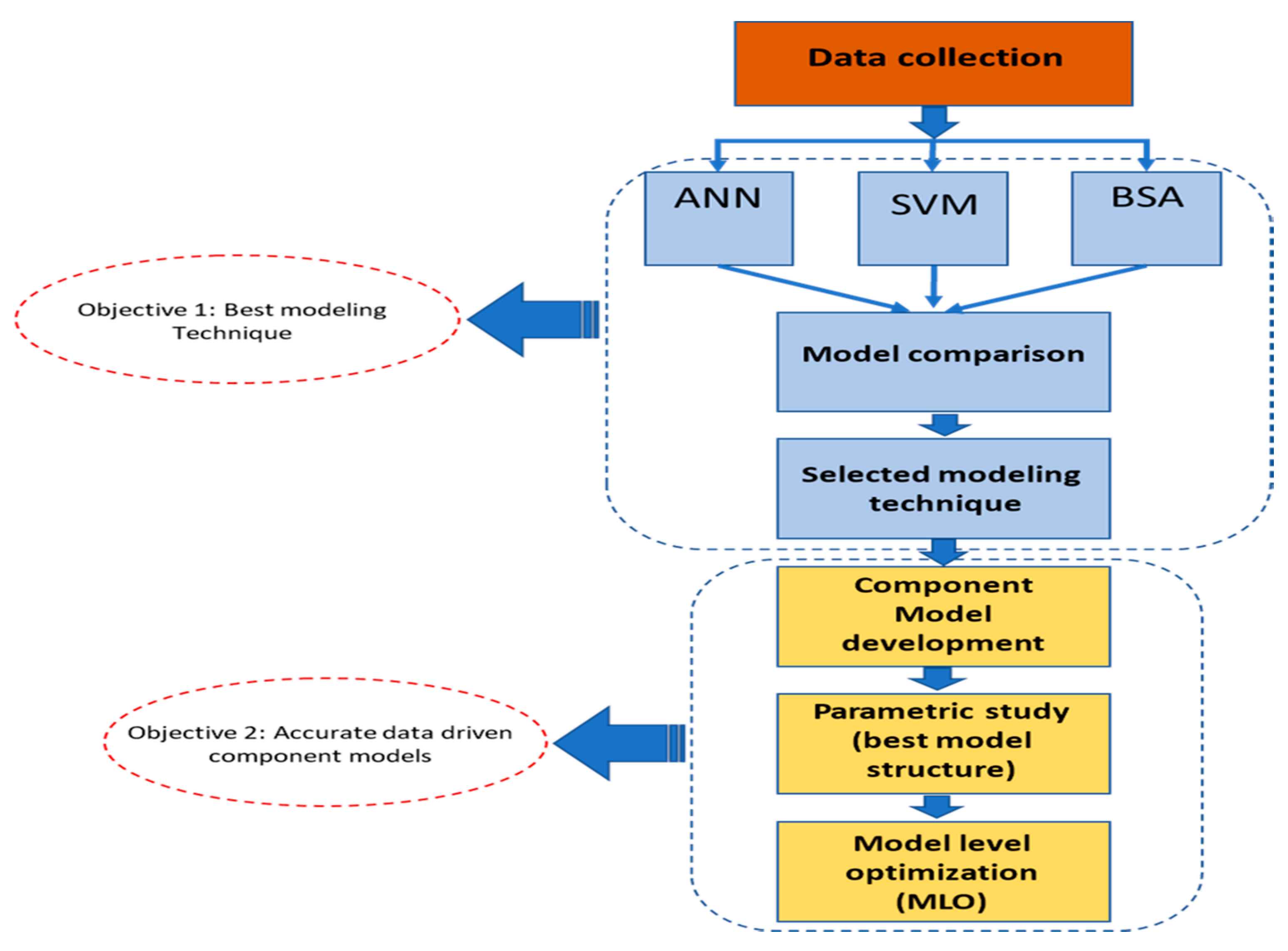
As previously stated, the HVAC systems are a complex nonlinear component. Therefore, the use of the optimization process to automate the process of selecting the best model structure became crucial. Because every component is different, it becomes hard to propose one model that can fit that component in all systems. Choosing the best model structure is a time-consuming process, and therefore the optimization process role in automating the process of selecting the optimal model structure for any individual component can be used. Moreover, choosing the best modeling tool will be crucial to model the HVAC systems. Therefore, this paper will have two objectives. The first objective is choosing the best modeling technique after comparing multiple proposed ones. The second objective is to create accurate data-driven component models using that selected tools. Figure 1 shows a general layout of the proposed modeling strategy. The proposed approach will be used to predict the performance of the components of the typical chilled water system and packaged DX systems. The proposed method had a limitation for this study in terms of model structure variables range, and that can be adjusted accordingly depends on the system under investigation.
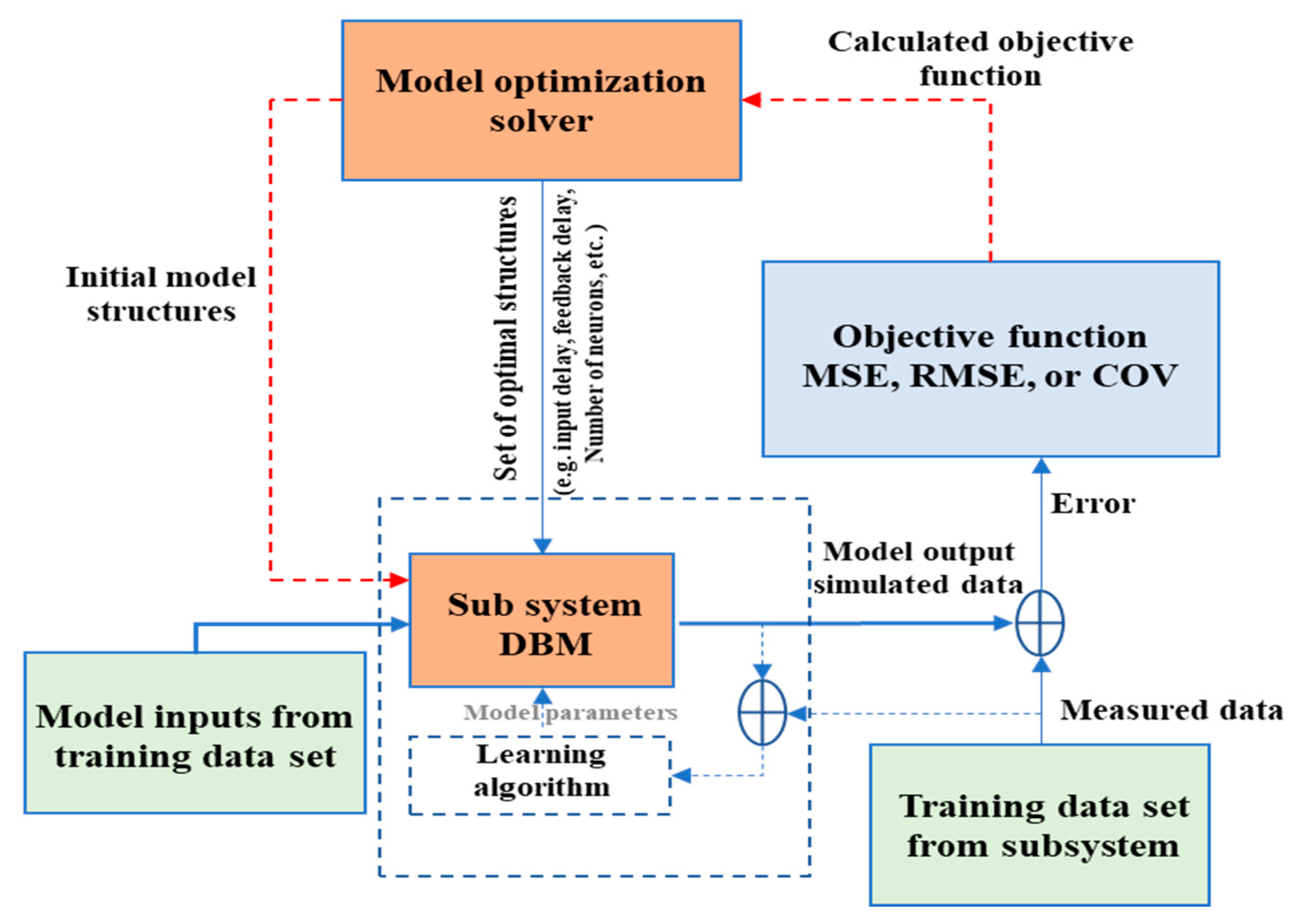
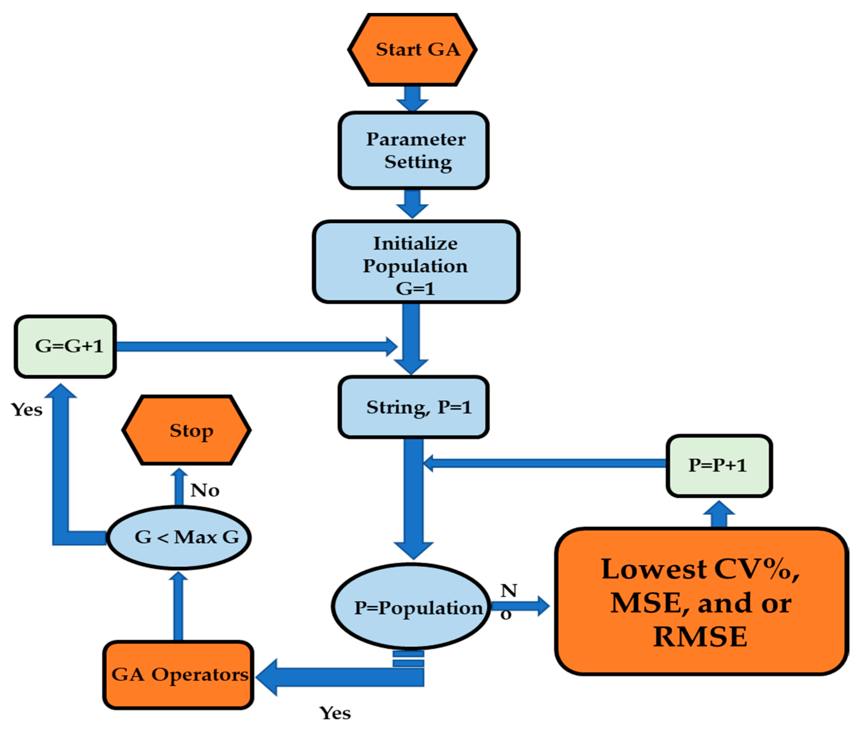
For the optimization process, there are two levels: one for model parameter tuning, where a typical learning algorithm is used; and the other one is the proposed calculations to determine the optimal model structures. For example, if an artificial neural network is used, the model structures are time delay, feedback delays, and the number of neurons. The model parameters are such as weights and biases. This process will perform a high-level optimization to select the best model structure by minimizing the error in model prediction. The error can be measured in terms of mean square error (MSE), root means square error (RMSE), and or the coefficient of variance (CV%). Figure 2 below shows the proposed optimization process. Where the model optimization solver starts with initial variables, the objective function is then calculated. This process repeats until the optimal variables yielding the least model errors can be found.
3. Modeling Description
The major component of the chilled water variable air volume (VAV) system air handling unit (AHU) and the packaged direct expansion (DX) systems were modeled. Table 1 shows the major components that will be modeled.
The models were examined to decide on the best model structure that held the highest accuracy value through a parametric study. For the cooling coil model, the supply air temperature was predicted as a function of (1) chilled water temperature, (2) chilled water valve position, (3) mixed air temperature, (4) supply airflow, and (5) mixed air humidity level. However, the fifth input (mixed air humidity ratio) was neglected for this study because there was not enough data collected to represent it. Moreover, for the fan model, the fan power was predicted as a function of fan airflow and fan speed. While for the DX system component models, the DX compressor was chosen to be modeled. Therefore, the compressor power for the DX system was predicted as a function of (1) outside temperature, (2) mixed air temperature, (3) airflow rate, and (4) moisture content mixed air.
To evaluate several data-based modeling techniques creating different models was proposed. Each model will utilize one of those techniques. The models will use the same inputs and output data to be tested and trained. Then the models will be compared, and the best-fitted model will be used selected as the modeling technique that will be used to carry on with this paper. Three predictive modeling techniques were chosen to be evaluated; those models were:
- Model (1): Support vector machine (SVM).
- Model (2): Artificial neural network (ANN).
- Model (3): Aggregated bootstrapping (BSA).
Support vector machine (SVM) is one of the methods that use supervised learning used for classification and clustering purposes. In general, SVM is also extended to solve regression problems, and thus support vector regression.
The main idea SVM is to reduce the dimensionality of a data set consisting of many variables correlated with each other, either heavily or lightly, while retaining the variation present in the dataset, up to the maximum extent.
While artificial neural networks (ANN) is a computational structure that is inspired by the observed process of the natural neurological networking of the brain. A key for these networks is their adaptive nature, where they essentially “learn by example” rather than by traditional programming methods [45,46]
Model three is utilized using bootstrap aggregation (BSA). Bootstrapping is simply the method of random sampling with replacement. Such a sample is referred to as a resampling [47]. Moreover, there may occur some redundancy in features that will later cause errors because high dimension data cost both speed and accuracy of the classification algorithms. Since the data were measured at very short intervals of time, the data set was large. So, there was a need to convert these high dimensional data into lower space to achieve better speed and accuracy [48]. To stop overfitting from happening, bootstrapping will be implemented.
To decide on the best modeling tool, the models will be tested and trained using the same data set. The selected tools will be compared through their fitness of predicting the same output. Training and testing are the primary two steps in creating any data-driven model.
- Training the models: Training is a phase in creating the machine learning models. A set of examples is used to fit the parameters of the model. The models are trained to entail an input and a corresponding output or target. The created model will be run with the training dataset and produces a result, which is then compared with the output or target for each selected input. Based on the results, the model parameters will be adjusted.
- Testing the models: Testing is the final phase after training. Where a dataset will be used to provide an unbiased evaluation of the final selected model from the training set. Generally, the dataset used for testing the models is different from the one used for training.
4. Model Evaluation Strategies
After the three models were tested and trained, how well the model fits the data was examined. There are a lot of statistical metrics that are available to test and validate the model performance. Like R2 (coefficient of determination), MSE (mean square error), RMSE (root mean square error), CV% (coefficient of variance), MBE (mean bias error), CVRMSE (coefficient of variance of root mean squared error), RN_RMSE (range normalized root mean squared error), etc. However, there will always be arguments that there is no conclusive statistical cut off criteria for model goodness-of-fit directories [49].
R2 is one of the model performance evaluation tools that is broadly used for model testing and validation [50]. R2 is better used to compare several models in terms of how good the model fits the data [44,51]. While, for example, RMSE is an error-index and often used as a measure to evaluate between two values predicted by a model and those observed from the thing that is being modeled [44]. When validating the building performance simulation models, the rule of thumb is to follow one of the main protocols like ASHRAE (American Society of Heating, Refrigerating and Air-Conditioning Engineers) Guideline 14, FEMP (Federal Energy Management Program), and IPMVP (International Performance Measurement and Verification Protocol) [52].
Moreover, both IPMVP (International Performance Measurement and Verification Protocol) and ASHRAE Guideline 14 indicate that R2 is the most important criterion by which a model’s validity and usefulness should be assessed. Therefore, in this paper R2 was used to examine the fitness of the model. R2, is the proportion of variation in the outcome values that is explained by the predictor variables (inputs).
In other words, R2 tells us how good the model fits the data (goodness of fit). The R2 value can range from 0 to 1. The higher the R2, the better the model. Where an R2 that is close to refers to a perfect fit while a value close to Zero or negative indicates a poor fit model [53]. An R2 value of 0.9 may be understood as 90% of the variance in the baseline is explained by the modeled values.
5. Data Collection
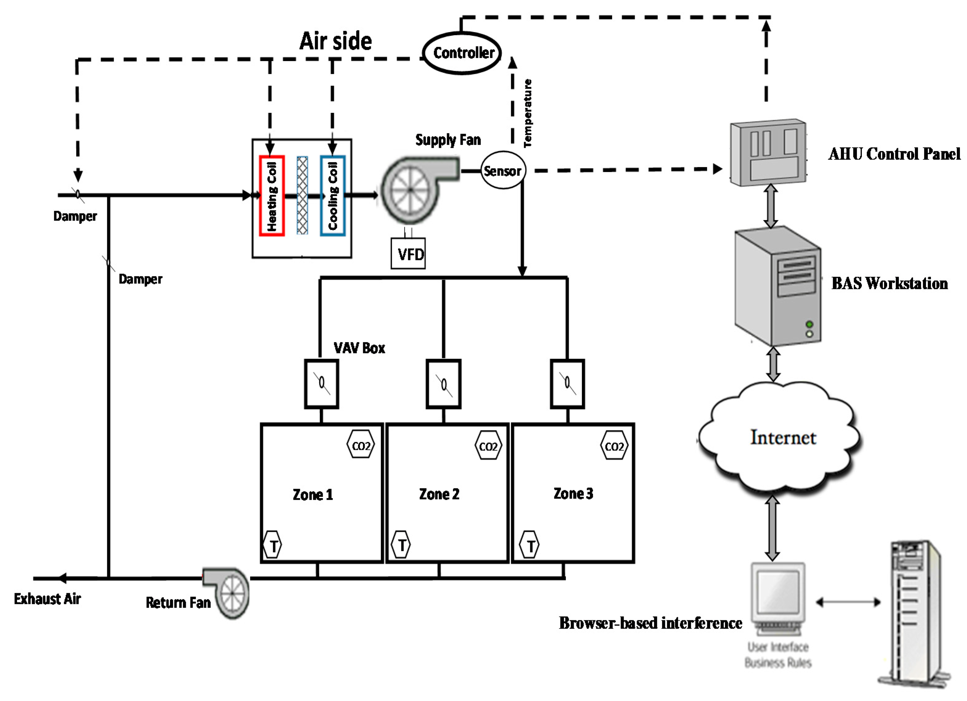
For the chilled water VAV system, real data gathered from an existing building located in North Carolina, USA. The building that covers 88,000 sf2 (464.5 m2) is a three-story multi-use building. The building is equipped with six AHUs and a chilled water planet with two chillers. Two AHUs are serving each floor. Additionally, the building is equipped with a building automation system (BAS) to record the performance of the building. Figure 3 shows a schematic of a typical VAV system layout and its correlation with the BAS. The data are collected on a span of one year.
The arrangement of each AHU consists of supply and return fan, exhaust, outside air dampers, heating, and cooling coils, VAV boxes, and multiple zones layout. The temperature range that was covered is a minimum of 50 °F (10 °C), and a maximum of 65 °F (18.3 °C), for the supply air temperature. The building is designed to have a supply air temperature (SAT) of 55 °F (12.8 °C). The data that were collected for this study to model the cooling coil successfully, as well as the fan model, are shown in Table 2 below.
However, for the DX system, an experimental set up was conducted in a fully equipped HVAC lab that is located at North Carolina A&T State University. The lab is equipped with 3-tons DX split-system air conditioning systems. The lab is controlled by a BAS that collects all the measurements data. The measurements that were recorded, as shown in Table 2, are outdoor air conditions, temperature, and humidity ratio entering and leaving the DX coil, airflow rates, damper positions, and compressor power.
Table 2 below shows the data that was collected and how they functioned as inputs and outputs for each model.
6. Selection of Modeling Tool Results
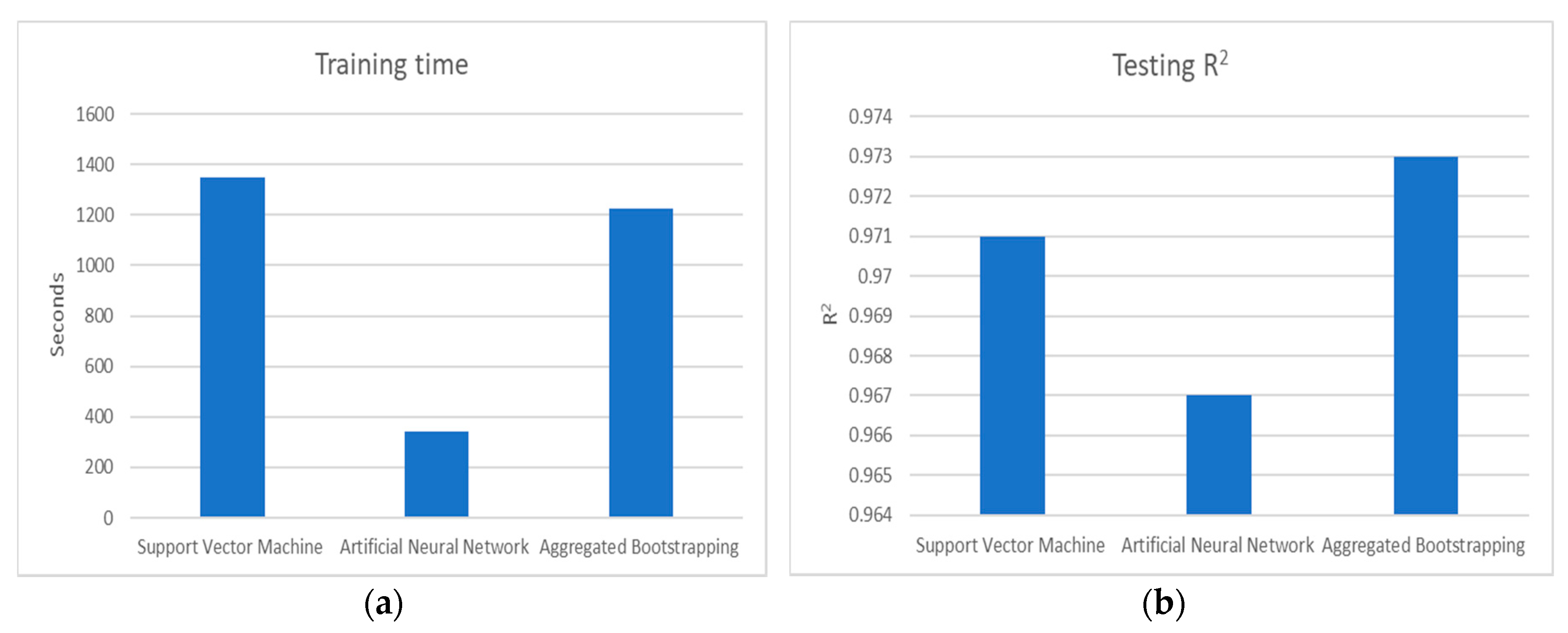
The selected inputs to feed the created models were chilled water temperature, chilled water valve position, mixed air temperature, and supply airflow. The output was the supply air temperature. Figure 2 shows that for predicting the supply air temperature based on the four inputs that were chosen in creating the model’s structure. The bootstrap aggregation achieved the highest R2 value for testing at 97.3%. Followed by the support vector machine and artificial neural networks with an R2 value for the testing period at 97.1% and 96.7%, respectively. However, when comparing the training time of the models. The artificial neural network had the lowest training time at 341.3 s, which is (less than 6 min). As shown in Figure 4, where the fitness values and the training time were plugged. All three models had a high R2 that is close in value. For the bootstrap aggregation model it indeed held the highest R2 value, but its training time was almost seven times as much as that for the neural network model. Moreover, the training time has increased with an increase in training set size.
From the results above, it was noticed that all three models held a high R2 value to train the specific dataset provided. However, the training time was the cutting edge in choosing the most suitable modeling tool. The artificial neural networks model was selected to be the modeling technique to model the performance of the cooling coil because it held the lowest training time comparing to the other models.
Therefore the ANN will be selected as the modeling technique that will be used to carry out this paper.
7. Parametric Study
Data-driven models that are based on real systems data are proven to be helpful tools in understanding the performance of HVAC systems and explain the relationship of the system components. Air handling units (AHU) are nonlinear systems, and it makes it hard to maintain thermal comfort. In this paper, the parametric study using ANN was conducted to predict the performance of the main components of any chilled water VAV system and DX systems; also, to validate the results of the optimization process that will be later conducted, through comparing the optimization results against the one generated through the parametric study.
The created model’s accuracy was tested in terms of MSE and CV%, which represents the error values of the models in predicting the actual performance. The model parameters that were adjusted in each iteration to get the best model structure are
- The number of hidden layers of neurons (N). For this investigation, the number of neurons that will be used ranges from 1 to 100.
- Feedback delay (FD). The FD in this study is measured by minutes. Each FD period is 5 min, and the total feedback delay is fifteen minutes.
- Time delay (ID). The ID is measured in minutes for this experiment, and to match the FD, the time delay will range from 1 to 3 intervals of 5 min for each interval resulting in a total of 15 min of delay.
An ANN is carried out using four steps: (1) extract the results or data, (2) train the network using experimentally or theoretically predicted values, (3) test the network with the data that are not used for training, and (4) identify the best network structure.
8. Model Level Optimization (MLO)
Today, modeling and simulation are established for addressing the problems related to the energy consumption in buildings. Energy performance modeling and optimization techniques and control strategies are gaining thrust in the research applications. Some of the available tools are not suited to be used for time-dependent applications. However, some artificial intelligence optimization tools are best suited for those applications since they have the compatibility to adjust optimal variables set points. Additionally, those tools are fast, adaptive, and capable of solving time-dependent algorithms related to the HVAC performance promptly.
Optimization refers to a process applied for minimizing or maximizing a function. The optimization algorithm will be implemented to automate the process by determining the best model structure with the minimum error value between the actual performance data and simulated data that were generated through the parametric study. The optimization tool that will be used to execute the optimization process is the genetic algorithm (GA). There are five phases in considering GA. Those processes are (1) initial population, (2) evaluation, (3) selection, (4) crossover, and (5) mutation. Figure 4 shows the optimization process using GA and how the five steps where implemented. Step (2), evaluation, was represented as the objective function. While steps 3, 4, and 5 are described as the GA operator. Figure 5 shows the process of the model optimization and objective function using the GA operator.
The error values were represented in terms of MSE (mean square error), RMSE (root mean square error), and or CV% (coefficient of variation), were those described in the following equations.
9. Results
A parametric study was conducted to understand better the performance of chilled water air handling units and DX packaged units. The relationship between the inputs and outputs is the parameter that will drive the results. The parametric study will generate a set of results for each iteration that the model was tested and trained. The results are transferred and organized, and the best model structure for each iteration was noted. However, for clarity of discussion, only the results of the titration that held the optimal model structure that held the absolute lowest error value are displayed. It is noted that when training the models, increasing the number of neurons has improved the accuracy of the prediction.
9.1. Cooling Coil Model Results
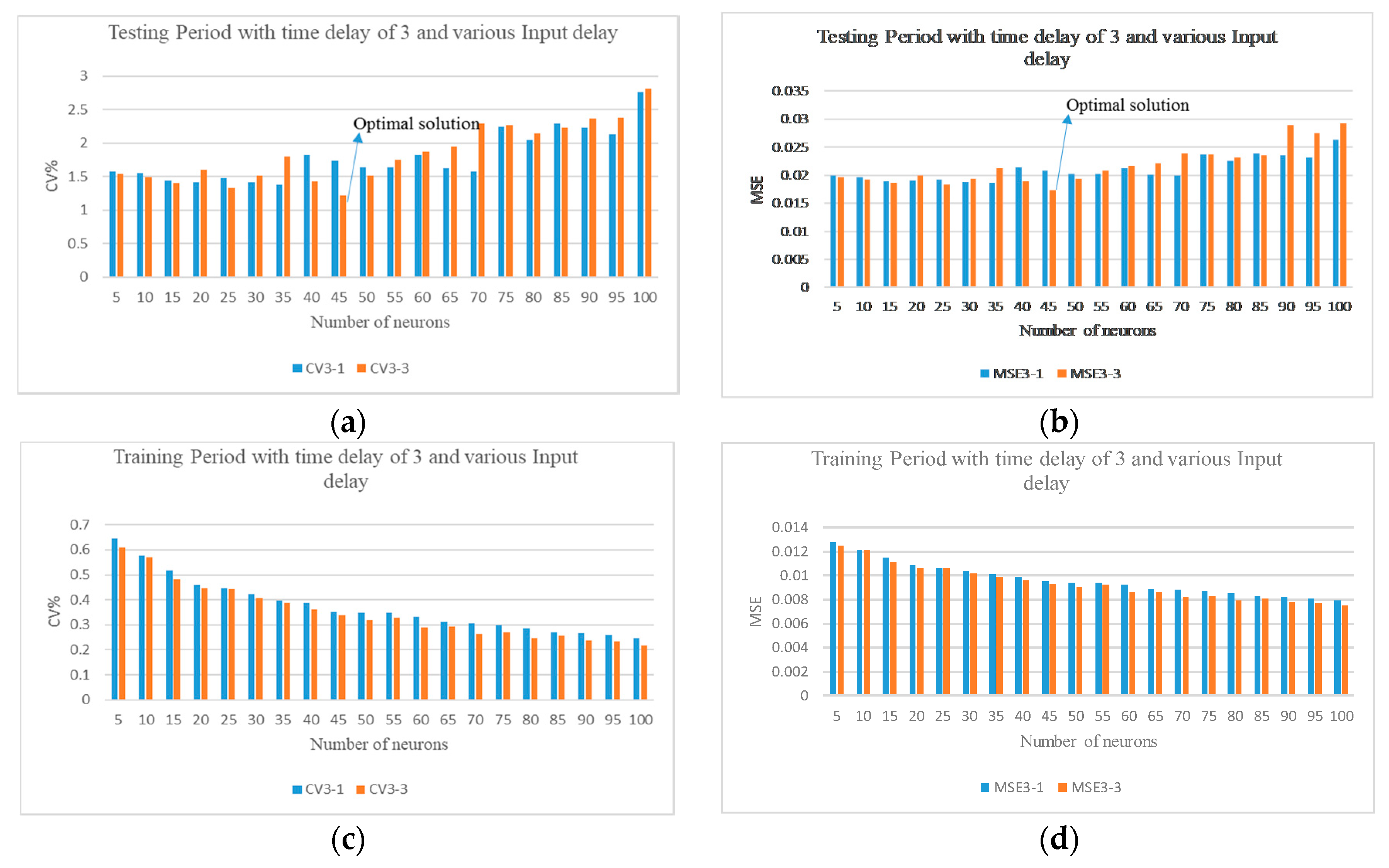
After conducting the parametric study and comparing all the results, the following results are for the cooling coil component. It was found that the model structure with 45 number of neurons, three intervals of feedback, and three intervals time delay held the least error values of 1.22% and 0.017 in terms of CV% and MSE, respectively. Thus, selected to be the best model structure in predicting the performance of the cooling coil, Figure 6 shows the testing and training period of a model with a number of neurons (N) ranging from 1 to 100 with a time delay (ID) of three intervals. This iteration held the optimal value.
9.2. Fan Power Model Results
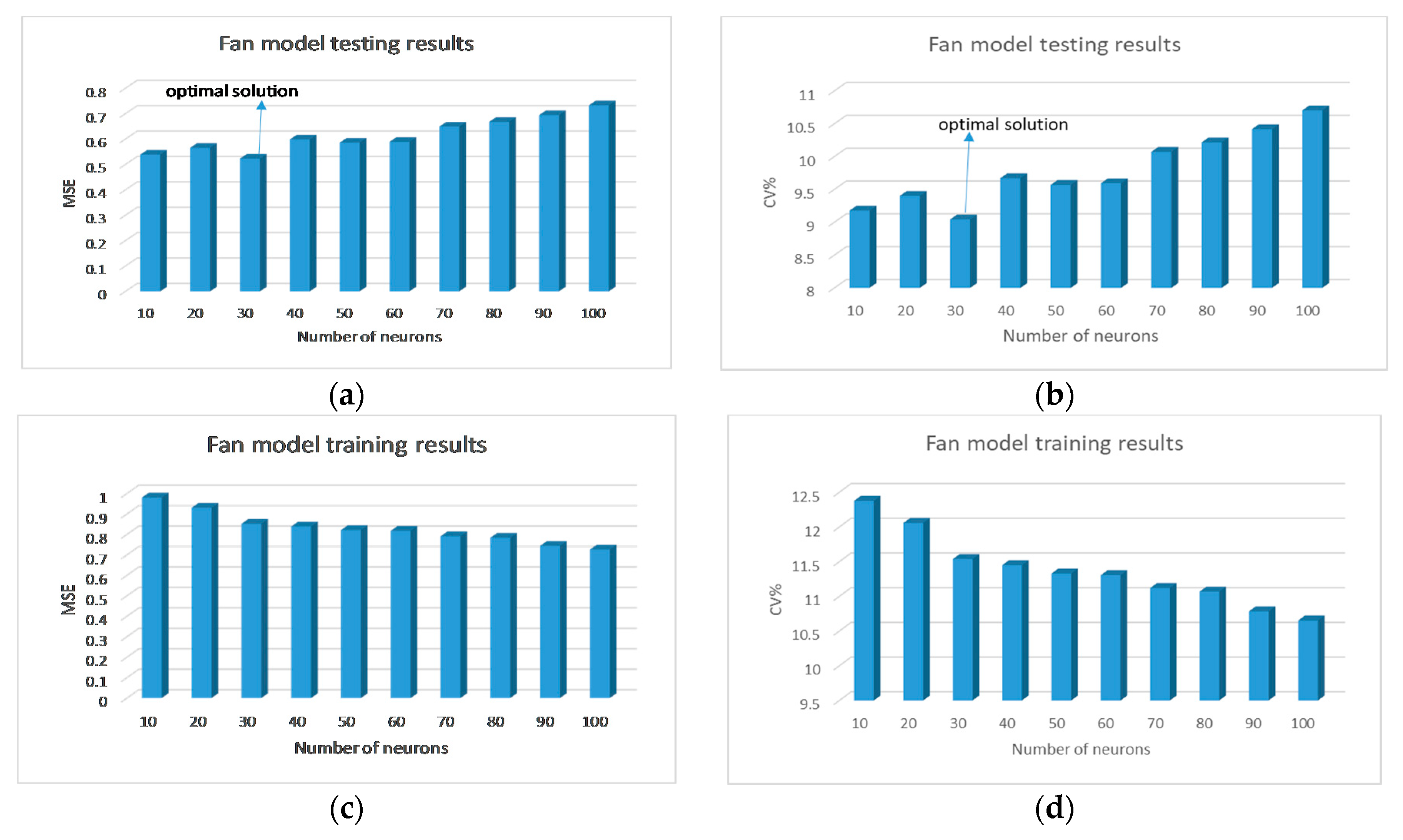
While for the fan power model, the same process was applied for the parametric study. The results have shown that the model structure with 30 number of neurons held the lowest error values. CV% and MSE values were recorded to be 9.04% and 0.523, respectively. This model is selected to be the best model structure for predicting the fan power usage of the AHU fan. Figure 7 shows the training and testing results for the iteration that held the optimal value.
9.3. DX System Model Results
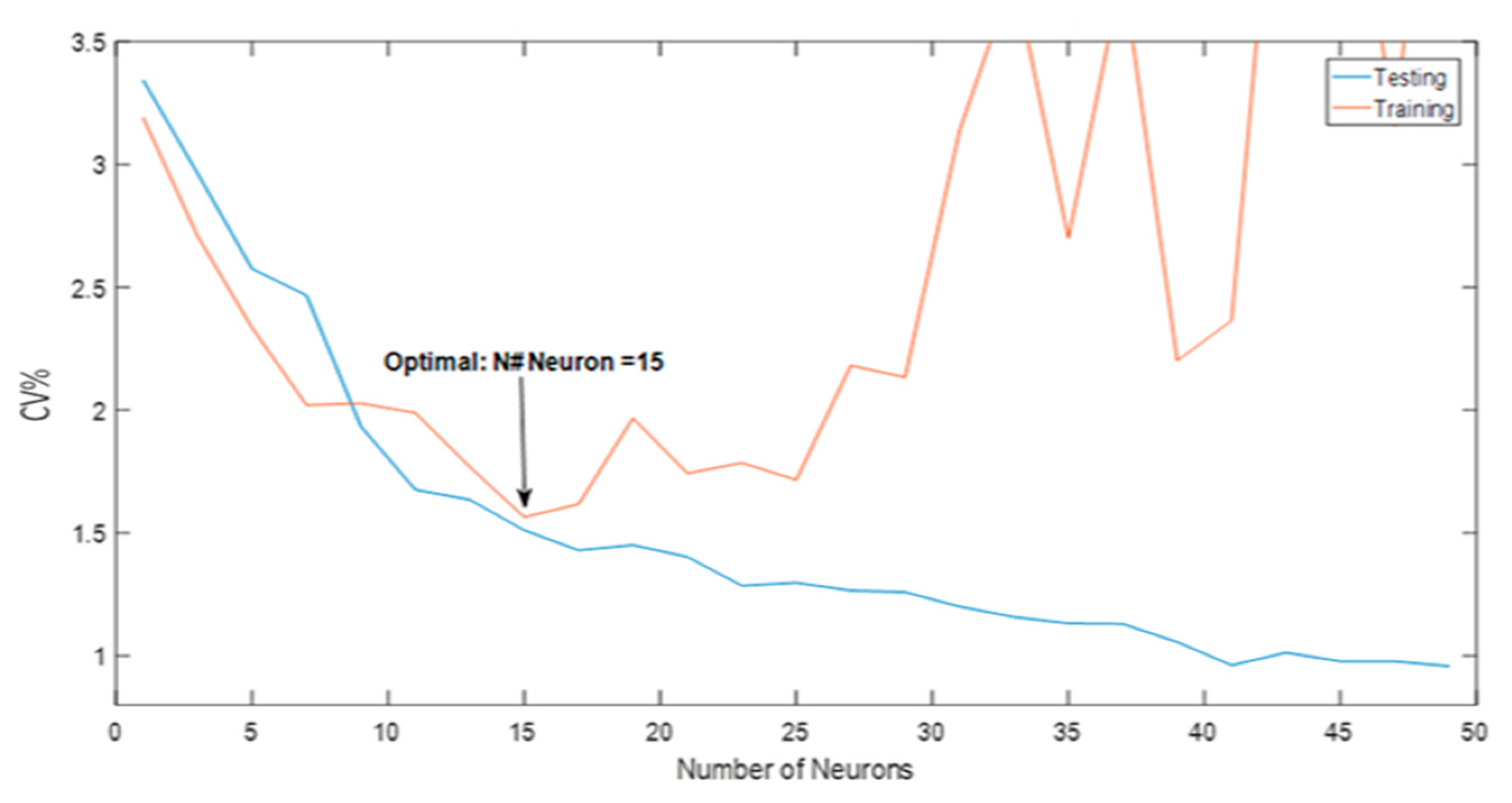
The results of testing and training the Dx system model have shown that the optimal model structure held a number of 15 neurons. The optimal iteration has held a CV% value of 1.54% for the training period. This model will be used as the best model in predicting the compressor power of the DX system. Figure 8 below shows the performance of the models in the training and testing period.
9.4. Model Level Optimization (MLO) Results
After the parametric study was deployed, the optimization technique using a genetic algorithm (GA) was conducted to automate the process of selecting the best model structure through minimizing the error between the actual and simulated data. The genetic algorithm was limited to a population size of 50 and a maximum of 100 generations. The optimization results will be compared against the parametric study results to validate the results. Table 3 and Table 4 show the results of the optimization process for each iteration. In Table 3, the results for the minimum CV% are displayed for the cooling coil. The moving average yielded the lowest CV% of 1.22%. Additionally, another genetic algorithm was created to predict the MSE value for each model structure. The results are shown in Table 3, where the lowest MSE yielded was 0.019. Therefore, the best model structure that can predict the cooling coil performance was at 45 number of neurons. The same process was repeated for the fan power model, and an optimization process using genetic algorithms was deployed. It was found that the best model structure that can accurately predict the fan power was at 30 number of neurons. The model with three intervals of delay yielded the lowest MSE and CV% values of 0.523 and 9.04, respectively.
It is noted that the results produced by the optimization tool are similar in value to those obtained in the parametric study. The optimization process has supported the parametric results where similar results were found. Furthermore, these results have proved that artificial neural networks can be a valuable tool in modeling the performance of CHW air handling components as well as the DX packaged systems components.
10. Conclusions and Future Work
In this paper, a data-driven optimization technique was proposed to optimize the performance of HVAC systems components (optimizing the component model structure) as part of the process of optimizing the whole system performance (optimizing the operation setpoints for the whole system).
The models predicted the performance of the cooling coil and fan as the major component of a chilled water variable air volume AHU and the compressor performance as the major component of the packaged DX system. Real data collected from a real building located in North Carolina, were used to train and test the proposed techniques. Several machine learning tools were compared to select the best modeling tool that will later be used to conduct a parametric study.
The tools that were chosen to be evaluated are support vector machine, artificial neural network, and aggregated bootstrapping. The R2 was used as the criteria of evaluation following the major code ASHRAE 14 guidelines. The tools were tested and trained on the same data set to examine the results better. However, all three modeling tools had close results in terms of R2. Therefore, the training time was also evaluated. The artificial neural network had a training time that was three times lower than both the other two. Therefore, artificial neural networks were chosen to be the tool to be a better modeling tool in modeling the components of the HVAC systems.
The optimization process using a genetic algorithm was conducted to select the best component model structure that held the lowest error value. Choosing the best component model structure is the first level of optimizing any HVAC system. Optimization of the performance of the HVAC system must be conducted on two levels. A component model optimization and system-level performance optimization. The two levels need to be integrated to be able to operate the HVAC system more efficiently and result in actual energy savings.
The genetic algorithm was used as the optimization algorithm to carry out this work. The optimization level results were compared against the one conducted through the parametric study, and similar results were found. Those results have shown GA to be a helpful tool in accurately predicting the performance of HVAC systems components.
The proposed data-driven modeling and optimization technique was proven to predict the performance of the investigated HVAC system components accurately.
Future work of the authors includes but is not limited to model the rest of the components of the selected HVAC systems. Models may include zone level, reheat, heat recovery, ventilation, etc. The models will be created and optimized using the data-driven optimization tool that is proposed in this paper after the tool was proven to be valid. Later, integrating all the component models and optimize the output of those models again to optimize the whole system setpoints (system-level performance optimization). The new optimized setpoints will be sent back to operate the system more efficiently. The period of optimization might be every 5–15 min. Optimizing the system setpoint is predicted to results in a more efficient system and eventually results in energy savings that will be calculated. The two levels will be tested in a fully equipped HVAC lab that is equipped with the discussed systems in the paper.
Author Contributions
Conceptualization, R.T. and N.N.; methodology, R.T. and N.N.; software, R.T. and N.N.; formal analysis, R.T. and N.N.; investigation, R.T. and N.N.; resources, R.T. and N.N.; data curation, R.T. and N.N.; writing—original draft preparation, R.T.; writing—review and editing, R.T.; visualization, R.T. and N.N.; supervision, N.N.; project administration, N.N.; funding acquisition, N.N. and W.C. All authors have read and agreed to the published version of the manuscript.
Funding
This work is partially supported by the Korea Agency for Infrastructure Technology Advancement (KAIA) grant funded by the Ministry of Land, Infrastructure, and Transport (20AUDPB099686-06).
Conflicts of Interest
The authors declare no conflict of interest. The funders had no role in the design of the study; in the collection, analyses, or interpretation of data; in the writing of the manuscript, or in the decision to publish the results.
References
- EIA. How Much Energy Is Consumed in Residential and Commercial Buildings in the United States? U.S. Energy Information Administration–Independent Statistics and Analysis: Washington, DC, USA, 2019.
- He, Q.; Ng, S.T.; Hossain, U.; Augenbroe, G.L. A Data-driven Approach for Sustainable Building Retrofit—A Case Study of Different Climate Zones in China. Sustainability 2020, 12, 4726. [Google Scholar] [CrossRef]
- Talib, R.; Nassif, N.; Arida, M.; Abu-Lebdeh, T. Chilled Water VAV System Optimization and Modeling Using Artificial Neural Networks. Am. J. Eng. Appl. Sci. 2018, 11, 1188–1198. [Google Scholar] [CrossRef] [Green Version]
- ASHRAE. ASHRAE Handbook Applications; American Society of Heating Refrigeration and Air Conditioning Engineers Inc.: Atlanta, GA, USA, 2011; Chapter 41. [Google Scholar]
- Beghi, A.; Brignoli, R.; Cecchinato, L.; Menegazzo, G.; Rampazzo, M.; Simmini, F. Data-driven Fault Detection and Diagnosis for HVAC water chillers. Control Eng. Pract. 2016, 53, 79–91. [Google Scholar] [CrossRef]
- Stanford, H.W. HVAC Water Chillers and Cooling Towers: Fundamentals, Application, and Operation, 2nd ed.; CRC Press: Boca Raton, FL, USA, 2011. [Google Scholar]
- Li, X.; Wen, J. Review of building energy modeling for control and operation. Renew. Sustain. Energy Rev. 2014, 37, 517–537. [Google Scholar] [CrossRef]
- Nassif, N. Modeling and testing of a single-speed DX air-conditioning system. ASHRAE Trans. 2018, 124, 44–51. [Google Scholar]
- Huh, J.-H.; Brandemuehl, M.J. Optimization of air-conditioning system operating strategies for hot and humid climates. Energy Build. 2008, 40, 1202–1213. [Google Scholar] [CrossRef]
- Afram, A.; Janabi-Sharifi, F. Theory and applications of HVAC control systems—A review of model predictive control (MPC). Build. Environ. 2014, 72, 343–355. [Google Scholar] [CrossRef]
- Afram, A.; Janabi-Sharifi, F. Black-box modeling of residential HVAC system and comparison of gray-box and black-box modeling methods. Energy Build. 2015, 94, 121–149. [Google Scholar] [CrossRef]
- Bell, A.A.; Angel, W.L. HVAC Equations, Data, and Rules of Thumb, 3rd ed.; McGraw-Hill: New York, NY, USA, 2015; Volume 40, pp. 394–398. [Google Scholar]
- Afroz, Z.; Shafiullah, G.; Urmee, T.; Higgins, G. Modeling techniques used in building HVAC control systems: A review. Renew. Sustain. Energy Rev. 2018, 83, 64–84. [Google Scholar] [CrossRef]
- Afram, A.; Janabi-Sharifi, F. Review of modeling methods for HVAC systems. Appl. Therm. Eng. 2014, 67, 507–519. [Google Scholar] [CrossRef]
- Talib, R.; Rai, P.; Nassif, N.; Tahmasebi, M. Modeling of Chilled Water VAV Systems Using a Machine Learning Approach. In Proceedings of the International Conference on Artificial Intelligence (ICAI). The Steering Committee of The World Congress in Computer Science, Computer Engineering and Applied Computing (WorldComp), Xuzhou, China, 22 August 2019; pp. 72–78. [Google Scholar]
- Kusiak, A.; Li, M.; Tang, F. Modeling and optimization of HVAC energy consumption. Appl. Energy 2010, 87, 3092–3102. [Google Scholar] [CrossRef]
- Arabali, A.; Ghofrani, M.; Etezadi-Amoli, M.; Fadali, M.S.; Baghzouz, Y. Genetic-Algorithm-Based Optimization Approach for Energy Management. IEEE Trans. Power Deliv. 2012, 28, 162–170. [Google Scholar] [CrossRef]
- Serraino, M.; Lucchi, E. Energy Efficiency, Heritage Conservation, and Landscape Integration: The Case Study of the San Martino Castle in Parella (Turin, Italy). Energy Procedia 2017, 133, 424–434. [Google Scholar] [CrossRef]
- MacLeod, M. SAVING ENERGY, SAVING MONEY; Businesses Are Cashing in, on Grants That Will Help Them Conserve Power; Spectator: Hamilton, ON, Canada, 2014. [Google Scholar]
- Mathew, P.A.; Dunn, L.N.; Sohn, M.D.; Mercado, A.; Custudio, C.; Walter, T. Big-data for building energy performance: Lessons from assembling a very large national database of building energy use. Appl. Energy 2015, 140, 85–93. [Google Scholar] [CrossRef] [Green Version]
- Turner, C.; Frankel, M.; Council, U.G.B. Energy performance of LEED for new construction buildings. New Build. Inst. 2008, 4, 1–42. [Google Scholar]
- Swaminathan, S.; Wang, X.; Zhou, B.; Baldi, S. A University Building Test Case for Occupancy-Based Building Automation. Energies 2018, 11, 3145. [Google Scholar] [CrossRef] [Green Version]
- Mills, E. Building commissioning: A golden opportunity for reducing energy costs and greenhouse gas emissions in the United States. Energy Effic. 2011, 4, 145–173. [Google Scholar] [CrossRef] [Green Version]
- Bouabdallaoui, Y.; Lafhaj, Z.; Yim, P.; Ducoulombier, L.; Bennadji, B. Natural Language Processing Model for Managing Maintenance Requests in Buildings. Buildings 2020, 10, 160. [Google Scholar] [CrossRef]
- EPA. Introduction to Indoor Air Quality; The United States Environmental Protection Agency: Washington, DC, USA, 2018.
- ASHRAE 62.1. Ventilation for Acceptable Indoor Air Quality; American Society of Heating, Refrigerating, and Air Conditioning Engineers Inc.: Peachtree Corners, GA, USA, 2016. [Google Scholar]
- Tam, C.; Zhao, Y.; Liao, Z.; Zhao, L. Mitigation Strategies for Overheating and High Carbon Dioxide Concentration within Institutional Buildings: A Case Study in Toronto, Canada. Buildings 2020, 10, 124. [Google Scholar] [CrossRef]
- Tse, W.L.; Chan, W.L. An automatic data acquisition system for on-line training of artificial neural network-based air handling unit modeling. Measurement 2005, 37, 39–46. [Google Scholar] [CrossRef]
- Reynolds, J.; Rezgui, Y.; Kwan, A.S.K.; Piriou, S. A zone-level, building energy optimisation combining an artificial neural network, a genetic algorithm, and model predictive control. Energy 2018, 151, 729–739. [Google Scholar] [CrossRef]
- Frausto, H.; Pieters, J.G.; Deltour, J. Modelling Greenhouse Temperature by means of Auto Regressive Models. Biosyst. Eng. 2003, 84, 147–157. [Google Scholar] [CrossRef]
- Ríos-Moreno, J.G.; Trejo-Perea, M.; Castañeda-Miranda, R.; Hernández-Guzmán, V.; Herrera-Ruiz, G. Modelling temperature in intelligent buildings by means of autoregressive models. Autom. Constr. 2007, 16, 713–722. [Google Scholar] [CrossRef]
- Kulkarni, M.R.; Hong, F. Energy optimal control of a residential space-conditioning system based on sensible heat transfer modeling. Build. Environ. 2004, 39, 31–38. [Google Scholar] [CrossRef]
- Meguro, W.; Peppard, E.; Meder, S.; Maskrey, J.; Josephson, R. Going Beyond Code: Monitoring Disaggregated Energy and Modeling Detached Houses in Hawai’i. Buildings 2020, 10, 120. [Google Scholar] [CrossRef]
- Mustafaraj, G.; Chen, J.; Lowry, G. Development of room temperature and relative humidity linear parametric models for an open office using BMS data. Energy Build. 2010, 42, 348–356. [Google Scholar] [CrossRef]
- Patil, S.; Tantau, H.; Salokhe, V. Modelling of tropical greenhouse temperature by auto regressive and neural network models. Biosyst. Eng. 2008, 99, 423–431. [Google Scholar] [CrossRef]
- Agbi, C.; Song, Z.; Krogh, B. Parameter identifiability for multi-zone building models. In Proceedings of the 2012 IEEE 51st IEEE Conference on Decision and Control (CDC), Maui, HI, USA, 10–13 December 2012. [Google Scholar]
- Li, Y.; Liu, M.; Lau, J.; Zhang, B. Experimental study on electrical signatures of common faults for packaged DX rooftop units. Energy Build. 2014, 77, 401–415. [Google Scholar] [CrossRef]
- Murphy, J. Energy-saving strategies for rooftop VAV systems: Control strategies can help turn energy savings into operating-cost savings and earn LEED credits. HPAC Eng. 2008, 80, 28. [Google Scholar]
- Stanke, D. Minimum Outdoor Airflow Using the IAQ Procedure. ASHRAE J. 2012, 54, 26–32. [Google Scholar]
- Yan, K.; Diduch, C.; Kaye, M.E. An Improved Temperature Prediction Technique for HVAC Units Using Intelligent Algorithms. In Proceedings of the 2019 IEEE Energy Conversion Congress and Exposition (ECCE), Baltimore, MA, USA, 29 September–3 October 2019; pp. 490–494. [Google Scholar] [CrossRef]
- Kim, S.-K.; Hong, W.-H.; Hwang, J.-H.; Jung, M.-S.; Park, Y.-S. Optimal Control Method for HVAC Systems in Offices with a Control Algorithm Based on Thermal Environment. Buildings 2020, 10, 95. [Google Scholar] [CrossRef]
- Nassif, N. Modeling and Optimization of HVAC Systems sing Artificial Neural Network and Genetic Algorithm. Int. J. Build. Simul. 2014, 7, 237–245. [Google Scholar] [CrossRef]
- Lin, C.-M.; Liu, H.-Y.; Tseng, K.-Y.; Lin, S.-F. Heating, Ventilation, and Air Conditioning System Optimization Control Strategy Involving Fan Coil Unit Temperature Control. Appl. Sci. 2019, 9, 2391. [Google Scholar] [CrossRef] [Green Version]
- Ahmad, M.; Mourshed, M.; Yuce, B.; Rezgui, Y. Computational intelligence techniques for HVAC systems: A review. Build. Simul. 2016, 9, 359–398. [Google Scholar] [CrossRef] [Green Version]
- Werbos, P.J. Beyond Regression: New Tools for Prediction and Analysis in the Behavioral Sciences. Ph.D. Thesis, Harvard University, Cambridge, MA, USA, 1974. [Google Scholar]
- Perez-Lombard, L.; Ortiz, J.; Pout, C. A review on buildings energy consumption information. Energy Build. 2008, 40, 394–398. [Google Scholar] [CrossRef]
- Breiman, L. Bagging predictors. Mach. Learn. 1996, 24, 123–140. [Google Scholar] [CrossRef] [Green Version]
- Khan, G.; Siddiqi, A.; Khan, M.U.G.; Wahla, S.Q.; Samyan, S.; Ghani, U.; Qayyum, S.; Waqar, S. Geometric positions and optical flow based emotion detection using MLP and reduced dimensions. IET Image Process. 2019, 13, 634–643. [Google Scholar] [CrossRef]
- Reddy, T.A.; Claridge, D. Uncertainty of “Measured” energy savings from statistical baseline models. HVAC&R Res. 2000, 6, 3–20. [Google Scholar] [CrossRef]
- Liang, J.; Du, R. Model-based Fault Detection and Diagnosis of HVAC systems using Support Vector Machine method. Int. J. Refrig. 2007, 30, 1104–1114. [Google Scholar] [CrossRef]
- Wang, C.C.; Sung, G.N. Low-power multiplier design using a bypassing technique. J. Signal Process. Syst. 2009, 57, 331–338. [Google Scholar] [CrossRef]
- Huerto-Cardenas, H.; Leonforte, F.; Aste, N.; Del Pero, C.; Evola, G.; Costanzo, V.; Lucchi, E. Validation of dynamic hygrothermal simulation models for historical buildings: State of the art, research challenges and recommendations. Build. Environ. 2020, 180, 107081. [Google Scholar] [CrossRef]
- American Society of Heating, Refrigerating and Air-Conditioning Engineers (ASHRAE). Guideline 14-2014. Measurement of Energy, Demand, and Water Savings; ASHRAE: Atlanta, GA, USA, 2014. [Google Scholar]
Figure 1.
A schematic of the modeling strategy.

Figure 2.
Proposed model level optimization strategy.

Figure 3.
Schematic of a typical chilled water variable air volume (VAV) system’s air handling unit.
Figure 3.
Schematic of a typical chilled water variable air volume (VAV) system’s air handling unit.

Figure 4.
Comparison of Models. (a) The training time for the three models in seconds; (b) the coefficient of determination (R2) value of the testing period for all the three models.
Figure 4.
Comparison of Models. (a) The training time for the three models in seconds; (b) the coefficient of determination (R2) value of the testing period for all the three models.

Figure 5.
The general layout of the optimization process using the genetic algorithm (GA).

Figure 6.
(a) Coefficient of variation (CV%) results for the testing period; (b) mean square error MSE results for the testing period; (c) CV% results for the training period; and (d) MSE results for the training period.
Figure 6.
(a) Coefficient of variation (CV%) results for the testing period; (b) mean square error MSE results for the testing period; (c) CV% results for the training period; and (d) MSE results for the training period.

Figure 7.
(a) MSE results for the testing period; (b) CV% results for the testing period; (c) MSE results for the training period; and (d) CV% results for the training period.
Figure 7.
(a) MSE results for the testing period; (b) CV% results for the testing period; (c) MSE results for the training period; and (d) CV% results for the training period.

Figure 8.
CV% results as a function of the number of neurons for the training and testing period of the DX model.
Figure 8.
CV% results as a function of the number of neurons for the training and testing period of the DX model.


Table 1.
List of the major component models.
| Data Based Models | Model’s Output | Description |
|---|---|---|
| AHU Model (Cooling Coil model) | Supply air temperature | This model will capture the performance of the cooling coil as the major component of the AHU |
| AHU Model (Fan power model) | Fan power | This model will capture the performance of the fan |
| DX Model (Compressor power) | Power | This model captures the performance of the compressor in a packaged DX VAV system |
Table 2.
The collected data and how they were divided into inputs and outputs for each model.
| Collected Data | Input and Output | Data Based Model |
|---|---|---|
| Supply airflow (CFM) | Input | AHU Model (Cooling Coil model) |
| Chilled water temperature (°F) | ||
| Chilled water valve position (°F) | ||
| Mixed air temperature (°F) | ||
| Supply air temperature (°F) | Output | |
| Supply fan speed | Input | AHU Model (Fan power model) |
| Fan air flow rate (CFM) | ||
| Supply pressure drop (in. w.g.) | ||
| Fan Power (kW) | Output | |
| outside temperature (°F) | Input | DX Model (Compressor power) |
| mixed air temperature (°F) | ||
| airflow rate (CFM) | ||
| moisture content mixed air | ||
| compressor power (kW) | Output |
Table 3.
Cooling Coil Model Optimization Results.
| Number of Neurons | Time Delay | Feedback Delay | Minimum CV% | Minimum MSE |
|---|---|---|---|---|
| 45 | 1 | 3 | 1.45 | 0.019 |
| 45 | 2 | 3 | 1.46 | 0.019 |
| 45 | 3 | 3 | 1.22 | 0.02 |
Table 4.
Fan Power Model Optimization Results.
| Number of Neurons | Delay Intervals | Minimum CV% | Minimum MSE |
|---|---|---|---|
| 30 | 1 | 9.32 | 0.555 |
| 30 | 2 | 9.04 | 0.523 |
| 30 | 3 | 9.075 | 0.527 |
© 2020 by the authors. Licensee MDPI, Basel, Switzerland. This article is an open access article distributed under the terms and conditions of the Creative Commons Attribution (CC BY) license (http://creativecommons.org/licenses/by/4.0/).
Share and Cite
MDPI and ACS Style
Talib, R.; Nabil, N.; Choi, W. Optimization-Based Data-Enabled Modeling Technique for HVAC Systems Components. Buildings 2020, 10, 163. https://0-doi-org.brum.beds.ac.uk/10.3390/buildings10090163
AMA Style
Talib R, Nabil N, Choi W. Optimization-Based Data-Enabled Modeling Technique for HVAC Systems Components. Buildings. 2020; 10(9):163. https://0-doi-org.brum.beds.ac.uk/10.3390/buildings10090163
Chicago/Turabian StyleTalib, Rand, Nassif Nabil, and Wonchang Choi. 2020. "Optimization-Based Data-Enabled Modeling Technique for HVAC Systems Components" Buildings 10, no. 9: 163. https://0-doi-org.brum.beds.ac.uk/10.3390/buildings10090163
Note that from the first issue of 2016, this journal uses article numbers instead of page numbers. See further details here.