
Detection of District Heating Pipe Network Leakage Fault Using UCB Arm Selection Method
by
Yachen Shen
1,2, 
Jianping Chen
2,3,*,
Qiming Fu
1,2,*,
Hongjie Wu
1,2,
Yunzhe Wang
1,2 and
You Lu
1,2 1
School of Electronics and Information Engineering, Suzhou University of Science and Technology, Suzhou 215009, China
2
Jiangsu Province Key Laboratory of Intelligent Building Energy Efficiency, Suzhou University of Science and Technology, Suzhou 215009, China
3
School of Architecture and Urban Planning, Suzhou University of Science and Technology, Suzhou 215009, China
*
Authors to whom correspondence should be addressed.
Buildings 2021, 11(7), 275; https://0-doi-org.brum.beds.ac.uk/10.3390/buildings11070275
Submission received: 10 May 2021
/
Revised: 17 June 2021
/
Accepted: 18 June 2021
/
Published: 27 June 2021
(This article belongs to the Collection Creation of a Low-Carbon Healthy Building Environment with Intelligent Technologies)
Abstract
:District heating networks make up an important public energy service, in which leakage is the main problem affecting the safety of pipeline network operation. This paper proposes a Leakage Fault Detection (LFD) method based on the Linear Upper Confidence Bound (LinUCB) which is used for arm selection in the Contextual Bandit (CB) algorithm. With data collected from end-users’ pressure and flow information in the simulation model, the LinUCB method is adopted to locate the leakage faults. Firstly, we use a hydraulic simulation model to simulate all failure conditions that can occur in the network, and these change rate vectors of observed data form a dataset. Secondly, the LinUCB method is used to train an agent for the arm selection, and the outcome of arm selection is the leaking pipe label. Thirdly, the experiment results show that this method can detect the leaking pipe accurately and effectively. Furthermore, it allows operators to evaluate the system performance, supports troubleshooting of decision mechanisms, and provides guidance in the arrangement of maintenance.
1. Introduction
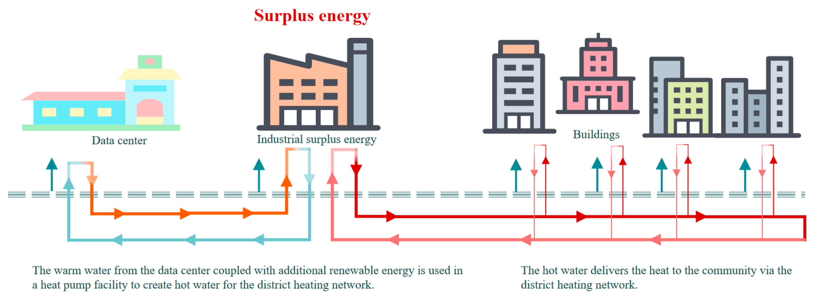
Intelligent fault detection is a very important part of future city digital development [1]. District Heating (DH) is an indispensable public energy service that transfers heat from heat sources to satisfy users who live in buildings [2]. A District Heating System (DHS) is shown in Figure 1 [3]. A DHS [4] is made up of three main components: heat sources, district heating networks, and substations. The temperatures of supply water and return water of the district heating networks (DHNs) are approximately 75–90 °C and 40–50 °C, respectively [5]. District heating networks distribute heat for residential and commercial heating purposes and domestic hot water in buildings. It is necessary to create a comfortable and pleasant indoor climate and guarantee the productive and domestic water [6]. Although DHSs can bring convenience to our lives, they will malfunction for several reasons. Even heat cessation may occur in severe cases. Heat cessation will cause severe harm to social activities and inhabitants’ lives. Accordingly, a reliable and online fault detection method should be applied to detect real-time faults.
Several problems may occur in the operation of DHNs as time goes on. Heat transfer causes temperature reduction. Friction of hot water against the pipe shell causes pressure losses. Both of these can lead to heat loss in the system. Moreover, pipe corrosion, insulation layer damage or fall off, leakage and other reasons may lead to pipe network malfunction. Among them, the phenomenon of hot water leaking from a damaged insulation layer or pipe shell cracking is common. Unfortunately, in existing DHNs, the observational data of leakage faults are relatively rare and cannot cover all leakage cases [7]. In order to obtain more data and realize online fault detection, it is necessary to simulate a district heating network, which can not only adapt to temperature fluctuations and user needs, but also anticipate component or entire system failures through fault detection and diagnosis (FDD). This will ultimately reduce costs for both utility companies and end-users.
In general, traditional FDD methods can be divided into: (1) signal processing-based methods; (2) analytical model-based methods; and (3) knowledge-based methods. These methods can achieve certain detection accuracies and basically detect these leakage faults, but they need large modeling efforts and lack accuracy and flexibility. Furthermore, with the development of artificial intelligence technology, a hybrid detection system combined with a variety of different intelligent technologies is the development trend of intelligent fault detection [8]. In the building pipe network, the sensors of pressure and flow are typically installed at each heat source, substation, and user terminal. In order to support the operation and maintenance of district heating systems, Supervisory Control and Data Acquisition (SCADA) systems can monitor and record running data in real time. Specifically, the leakage fault of DHSs will cause slight changes in the flow and pressure parameters compared with normal circumstances, which inspires researchers to locate leakage faults through these subtle changes. Based on this point, several leakage fault detection (LFD) methods have been implemented to locate leakage points. Zhao et al. [9] studied the leakage detection and location of natural gas pipelines based on negative pressure and combined the negative pressure wave method with the signal theory to propose a solid part method to find the singularity. In order to locate the leakage, the gas velocity in the Romberg and the Dichotomy Searching methods are considered in the location formula. Jia et al. [10] provided a new pipeline leakage location method that combined the advanced FBG circumfluence strain sensor with an effective classification algorithm based on a BP neural network. Xue et al. [11] proposed a machine learning-based detection method for heating pipe network leakage by establishing a hydraulic simulation system to obtain a leakage dataset, adding a strong integrated algorithm, XGBoost, to the model, which finally outputs the leaking pipe label. Lei et al. [12] used a BP neural network to detect leakage faults both in a branch-shaped heating network and loop-shaped heating network. At the same time, he also used an SVM to make improvements. Morteza et al. [13] proposed a leakage detection method based on Artificial Neural Networks (ANNs). Berg et al. [14] proposed using a thermal image enhancement analysis method to reduce the number of false alarms in the leakage of heating networks. Most of the pipe network LFD methods discussed above focus on wave detection or supervised learning. The DHN is a closed circulation network consisting of an equal number of supply and return pipes. However, due to the cost problem, in most cases, there are not enough sensors to monitor all pipes’ situations. Thus, more efficient LFD methods are necessary. A reliable LFD method for DHNs ought to have three features: high accuracy, low investment, and online and real-time detection capabilities.
Reinforcement learning is the closest to the human learning style in machine learning, which provides an alternative solution for the fault detection of a smart city energy system. Reinforcement learning is a powerful unsupervised learning method in which the environment gives agent feedback and the agent selects the optimal action with the goal of obtaining the maximum expected cumulative reward [15]. Based on the idea of “only using the current state to obtain the optimal action” in reinforcement learning, this paper proposes a method for the rapid online detection of pipe network leakage faults based on Contextual Bandit [16,17]. In this paper, reinforcement learning is used to carry out some exploratory research in the field of pipe leakage fault detection. The results show that the fault detection accuracy is improved, and our method has a high adaptability for different pipe networks. Moreover, the proposed method does not depend on the model of the problem. Based on the collected sensor data, it can perform the online training automatically. Thus, it also features low investment and online real-time detection capabilities. Three main components of this research are summarized as follows.
- A reinforcement learning-based approach needs a large number of samples associated with all possible leakage fault situations. Unfortunately, in existing district heating networks, the observational data of leakage faults are relatively rare and cannot cover all leakage cases. Therefore, the hydraulic simulation model established by Xue [11] is used to obtain a leakage dataset [18]. In order to ensure the accuracy of the results, an impedance identification method was also used;
- When a malfunction occurs, the overall DHN make-up water will often change greatly, which will trigger the alarm. In order to enhance system robustness, a delayed alarm triggering algorithm is applied to check the make-up flow rate regularly to indicate whether a leakage has occurred;
- The core of the leakage fault detection model is Contextual Bandit (CB). It mainly includes model parameter synchronization, model prediction, an exploitation–exploration mechanism, real-time feature recording and storage, etc. The model uses the observed data as states to indicate agent arm selection which is a leaking pipe label.
2. Theoretical Background
2.1. Contextual Bandit
In probability theory and machine learning, the multi-armed bandit problem (also called the K- or N-armed bandit problem) is a problem to which a fixed set of finite resources should be allocated among different choices to maximize the cumulative expected payoff. This is a typical reinforcement learning problem, which reflects the exploration–exploitation tradeoff dilemma. The gambler must decide which machines to play, how many times to play each machine and in which order to play them, and whether to continue with the current machine or try a different machine. In this problem, each machine provides a random reward based on a probability distribution specific to that machine. The gambler goal is to maximize payoff through a series of lever pulls.
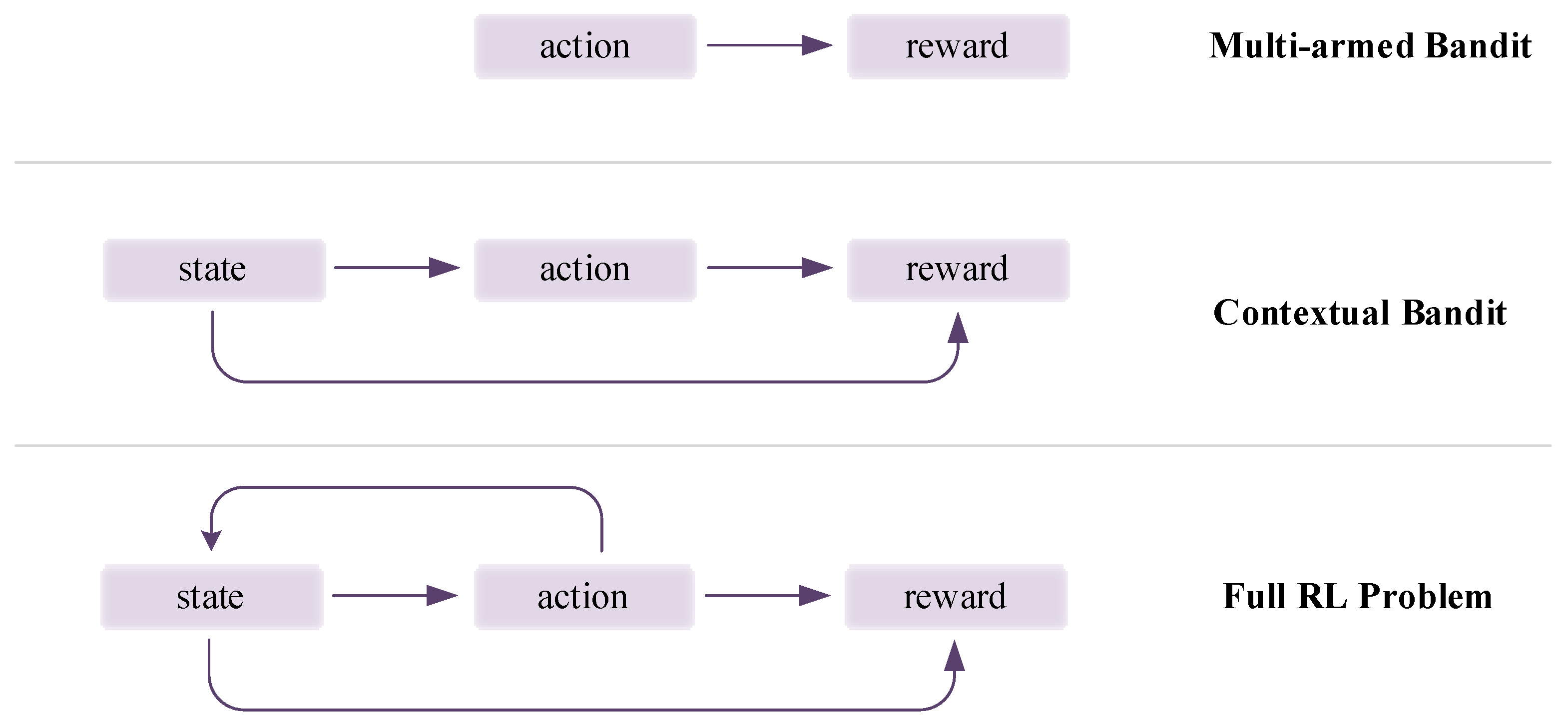
Figure 2 compares the relationship between the state and the action in different bandit algorithms. In the top subfigure, as a multi-armed bandit problem, the reward is only affected by the action. In the middle one, the contextual bandit problem, both states and actions can affect the reward. Additionally, in the bottom one, a full RL problem, the next state will be affected by the action, and the reward will be affected by both states and actions and it will also be delayed at the same time [19].
In a multi-armed bandit problem, the agent picks a pull from multiple arms of that bandit, and a payoff corresponding to the value between 0 and 1 is obtained. The problem is considered solved when the agent always chooses the arm that can return a relatively large payoff. In this case, the agent completely ignores the state of the environment, as there is only a single unchanging state [20].
In a contextual bandit problem, at each iteration, based on a state and the rewards of the arms played in the past, which is often represented as a d-dimensional eigenvector (contextual vector), an agent can choose which arm to play with. In the learning process, the agent has to try to collect more and more information, which is about the relationship between the state and the reward. In this way, it can choose the best arm to pull according to the current state [21].
LinUCB is an online linear method of Contextual Bandit. The basic idea is to assume a linear relation between the expected reward of an action and its contextual state, and a set of linear predictors is also used to model the representation space [22].
2.2. Upper Confidence Bound (UCB)
Rather than performing the exploration by simply selecting an arbitrary action, it is better to define a heuristic information formula for the arm selection. The UCB algorithm uses uncertainty in the action-value estimations for balancing exploration and exploitation. With UCB, At, the action selected at time step t, is:
where t denotes the total operational numbers of each arm currently; denotes the number of times action a has been selected before time t, and c is a confidence value that controls the level of exploration. If , a is considered as the most likely action to be chosen.
Equation (1) can be thought of as being formed from two distinct parts. represents the exploitation part. UCB is based on the principle of “optimism in the fact of uncertainty”, which basically means if you do not know which action is best, then select the one that currently seems to be the best—that is, the action with the highest estimated reward will be selected.
The second half of the equation represents the exploration, where the degree of exploration is controlled by hyper-parameter c. Effectively, this part of the equation provides a measure of the uncertainty for the action’s reward estimation. If an action has not been selected frequently, or has not been selected at all, then will be very small. Therefore, the uncertainty term will be large, which will make this action more likely to be selected. Every time an action is taken, the agent become more confident about its estimation. In this case, increases, and so the uncertainty term decreases, which will make it less likely to be selected as exploration (although it may still be selected as the action with the highest value, mainly due to the exploitation term). When an action is not being selected, the uncertainty term will grow slowly, due to the ln function, whereas every time that the action is selected, the uncertainty will decrease rapidly due to the increase in . Gradually, the exploration part decreases (since goes to infinity, the square root term goes to zero), and eventually actions are selected based only on the exploitation part [23].
3. LFD Method Based on Reinforcement Learning
3.1. Delayed Alarm Triggering Algorithm
The amount of make-up water is used to measure whether a leakage has occurred. Nevertheless, due to the influence of measurement error and environmental noise, an instantaneous peak value will inevitably appear [24]. Inspired by electric power systems, this paper uses a delayed alarm triggering algorithm to reduce the effects of these interferences.
It is not recommended to trigger the alarm signal immediately when the amount of make-up water just exceeds the threshold value (typically set to 1% of the total circulating flow rate ). The maximum tolerance M (typically set to ) acts as a buffer. When the buffer is full, the alarm will be triggered. For each check, the maximum observed value can be set according to the sampling interval. The simulation systems often set the sampling intervals to less than 10 min. Thus, waiting for several succussive observations can reduce the disturbance of measurement errors and noise, which makes the algorithm more robust.
3.2. CB-Based Leakage Fault Detection
3.2.1. Fault Detection Process
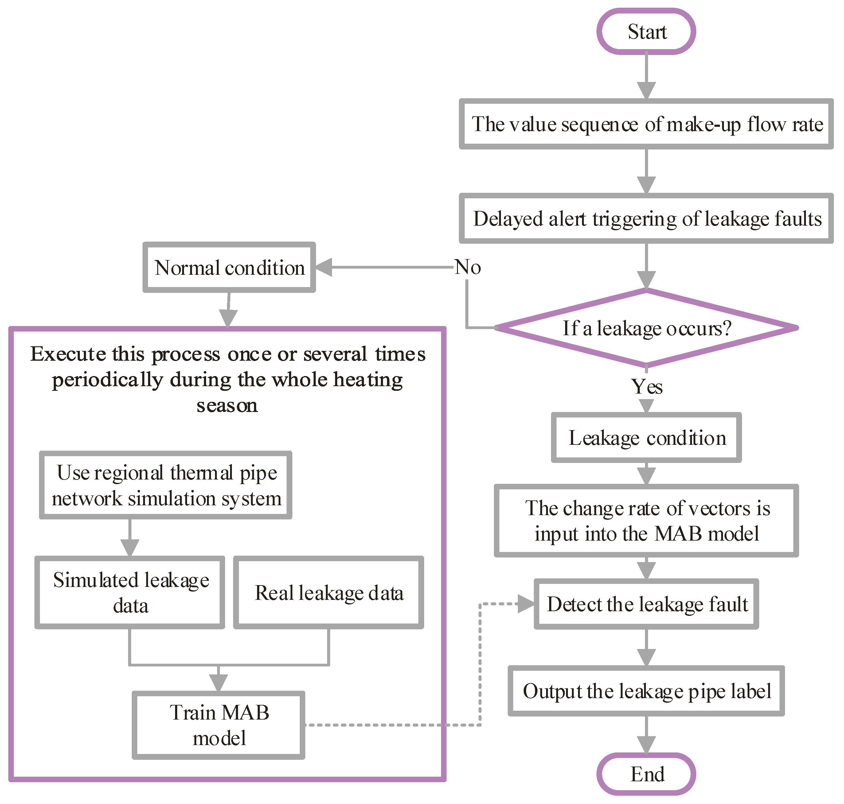
Figure 3 shows the leakage fault detection process using the Contextual Bandit algorithm. Firstly, the establishment of a small DHN pipe network is used for simulating all leakage faults that can occur in the networks, which can be used to construct a dataset. Then, the simulated leakage data and real leakage data are used to train a CB model. Secondly, when the amount of the overall network make-up water exceeds the threshold, the alarm system will not be triggered until the buffer is full. It can effectively mitigate the interference of measurement errors and noise. Finally, when the leakage occurs, the observed data are sent to the CB model for the best arm selection, which is the leaking pipe label [25].
3.2.2. LinUCB for Disjoint Linear Model
This method solves context-independence problem in a traditional MAB and considers the influence of the state on arm selection.
We assume that the expected payoff of an arm a is linear in the d-dimensional feature , with some unknown coefficients vector —namely, for all t:
where is the contextual information, i.e., the information about the eigenvectors of a pipe network. The parameters of the model are not shared among different arms. Each arm has a set of weights with a weighted relationship to the d-dimensional features to obtain the expected payoff. Considering the total loss function of multiple experiments on a single arm, we define the square loss function as follows:
We use the L2 regularization to prevent overfitting, where is the identity matrix. By making the derivative of in Equation (3) equal to zero, we obtain:
Let Da be a matrix at trail t, where the rows correspond to m training inputs, and is the corresponding reward vector. Since it is an extension of the UCB method, in addition to obtaining the expected value, we also need a confidence upper bound. Fortunately, an upper bound has been found that is at least [26].
where is a constant, for any as well as . The UCB arm selection strategy can be obtained from the inequality above. At each trial t, choose:
where ,.
Ridge regression can also be seen as a Bayesian point estimate, where the posterior distribution of the coefficient vector, denoted as , is a Gaussian with mean and covariance . The predicted variance of the expected payoff is evaluated as , and then becomes the standard deviation. Moreover, in the information theory, the differential entropy of is defined as . The entropy of is updated with the addition of the new point . Then, it becomes . The entropy reduction in the model posterior is . The contribution from is evaluated by this quantity for model improvement. Therefore, the arm selection criterion in Equation (7) can also be seen as a tradeoff between the payoff estimation and reduction in the uncertainty in the model [27].
3.2.3. Algorithm Design
Firstly, the datasets measured by the sensors are processed by splicing into matrixes, which are regarded as different state spaces Da in CB. There are n flow sensor data , and m − n pressure sensor data , which are combined to form , modeled as states in RL. a pipes can be modeled as actions in RL. The arm selection in CB is just the action selection, which also means locating the leakage pipe in DHS, . The reward function is set to , where corresponds to a normal distribution function between 0 and 1. Additionally, the leaking pipe corresponds to the maximum value of . Iteratively updating the A and b values is carried out to update the weights . The overall algorithm is shown in Algorithm 1.
| Algorithm 1. Leakage fault detection algorithm based on Contextual Bandit |
| flow and pressure sensor data. |
| , total mass flow of replenished water |
| , flow threshold, set to 10% of |
| , maximum number of observations in one inspection |
| Output: a, selected action (select a leaky pipe) |
| (a) loop |
| (b) initialize , , s = false, M = 0.5 N0 |
| (c) for t = 1,2,…, N0 do: |
| (d) if s = false then: |
| (e) if : |
| (f) if : s = true |
| (g) break |
| (h) else: |
| (i) else for t = 1,2,3,…: |
| (j) get the current contextual association vector for all arms |
| (k) for all a: |
| (l) if a is new: |
| (m) set Aa to d-dimensional unit matrix |
| (n) set ba to d-dimensional zero vector |
| (o) calculate |
| (p) calculate arm selection probability |
| (q) update |
| (r) update |
4. Experimental Analysis
4.1. Model Parameters
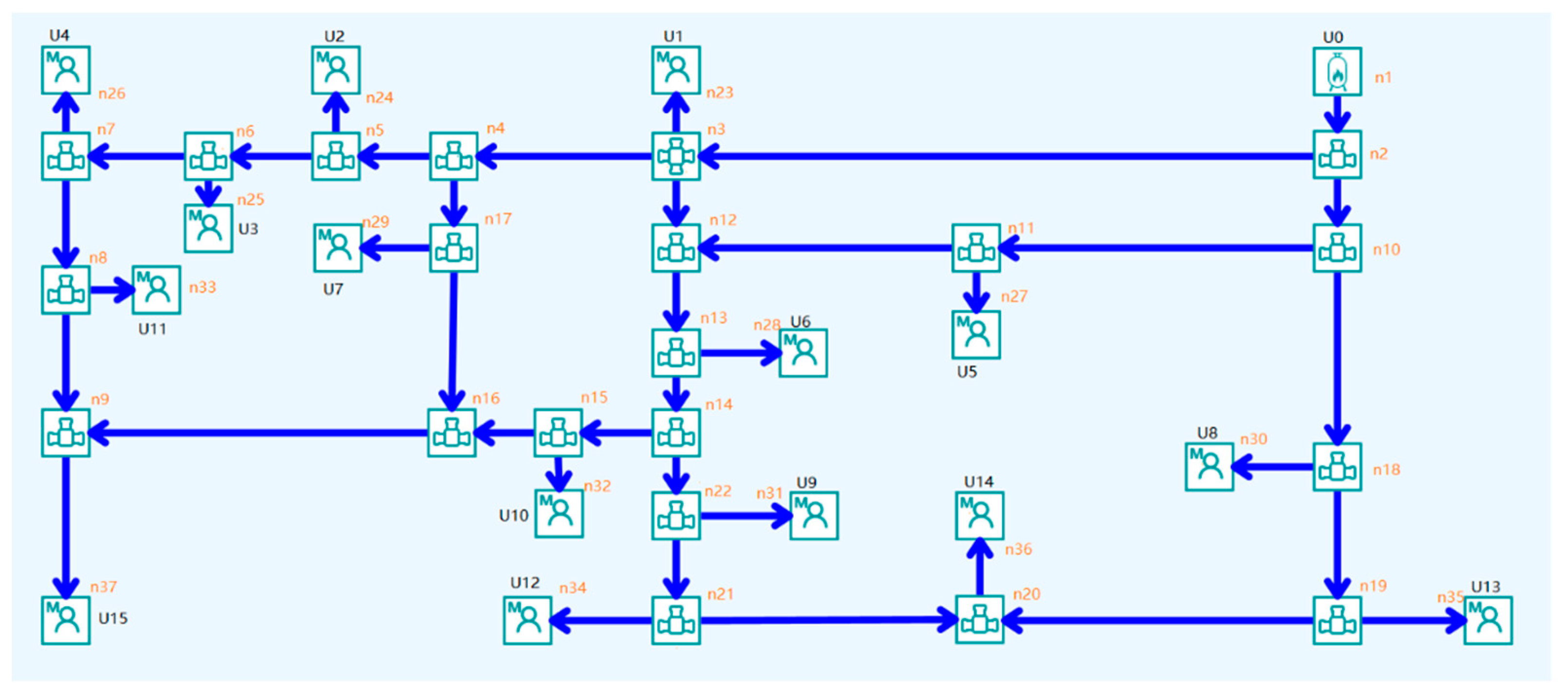
There are 16 users in our simulation model. The flow parameters of each pipe in the simulation model are given in Table 1.
We used the stratified sampling method to divide the leakage dataset into a training set and a test set. In total, 70% of the whole leakage dataset was used as the training set and the rest were used as the test set. Table 2 shows the design information and data quantity of the pipe network.
4.2. Evaluation Criteria
In order to implement the LinUCB algorithm for the given dataset, we first parsed each line of the input text file in the following way:
- Strip every line of new line character;
- Iterate over each line of input, which act as individual time steps, and split the line based on a single space. This gives us a list of 48 elements;
- Pop the head of the list and assign it as the arm for the current step;
- Take the remaining 47 elements and assign them to the context array for the current step.
This gives us all the parameters required to perform the online reward prediction of the arms [29].
Then, with all the required parameters, we calculated the coefficient, payout and standard deviation for each arm at every step and chose the arm with the highest payoff (i.e., upper confidence bound) as our selection. This prediction was followed by an update of matrixes “A” and “b” for the predicted arm. This was repeated for all time steps.
In order to evaluate the accuracy of our algorithm, we used the cumulative take-rate replay which at time T is defined as:
Whenever the selected arm is equal to the current arm, the identity function evaluates to 1 and the CTR is updated for that time stamp [30].
4.3. Analysis of Experimental Results
4.3.1. Comparison with Other Methods
At present, supervised learning methods are mainly used for pipe network fault leakage detection, such as XGBoost, forward neural networks, and support vector machines, etc. XGBoost is an optimized version of gradient tree promotion, which has had a good effect on multi-classification tasks. In the application scenario of this paper, the classification accuracy of XGBoost can reach 86.55% [11], the traditional BP network and SVM only reach 85% [12], and the accuracy of improved support vector machine can reach 92% [13].
Specifically, we consider a dynamic environment and apply the learned model to each new leakage pipe situation. It can perform experiments in the environment, obtain samples online, extract experience from the experiments, and modify the weights θ according to the tendency of past pipe damage. Our method, compared with other supervised learning methods (1) can acquire samples online without manual labeling and (2) enables online learning and has greater adaptability to new changes.
In the training phase, since reinforcement learning searches in a large space, the convergence speed is slower than that of neural networks. In practice, for example, the online learning characteristics of reinforcement learning make the speed of convergence depend on online sample acquisition. After the model stabilized, the Contextual Bandit algorithm supports the addition and deletion of dynamical candidate pipes. When a new pipe is added, it will be initialized in real time, added to the arm selections, given a certain exploration rate. In contrast, the neural network-based multi-classification approach has to add an input to the input layer, retrain the neural network, and correct the weights when a new pipe is added.
A comparison of accuracy rates of the different research methods is shown in Table 3.
Although the fault detection algorithm proposed in this paper has a slower convergence time than other supervised learning methods. However, our method can realize online learning, support the addition and deletion of new pipes, and improve the accuracy at the same time. This is extremely helpful for DHN companies and end-users.
4.3.2. Arm Selection Analysis
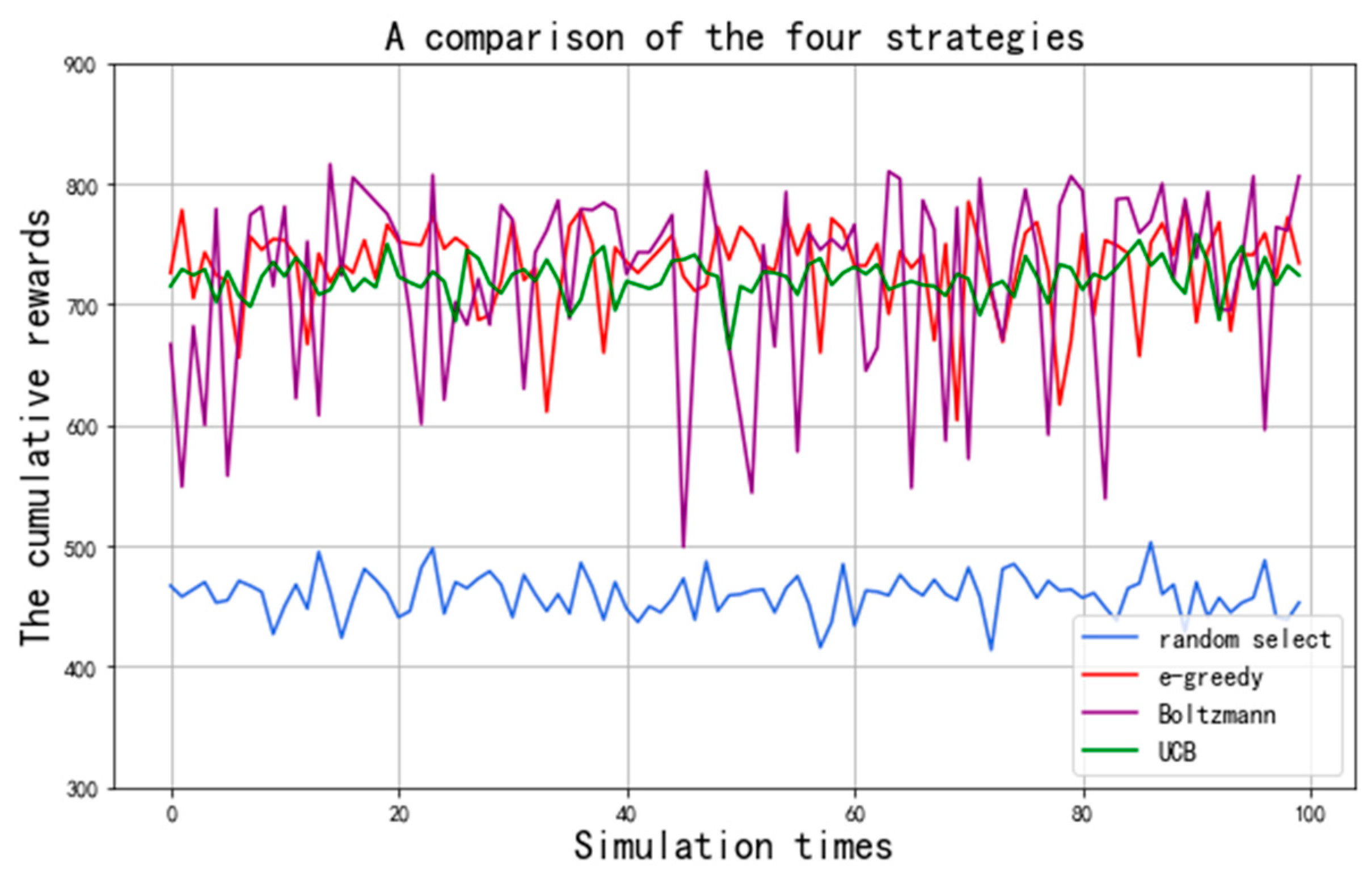
As shown in Figure 5, the UCB method is compared with the random selection method, ε–greedy method, and the Boltzmann method. After comparing these four methods, we found that the randomly selection method has the worst performance and the other three methods have a small difference in cumulative reward. However, the UCB strategy fluctuates less and is very stable, which not only guarantees the accumulation of rewards, but also an accurate estimate of the real rewards of each arm.
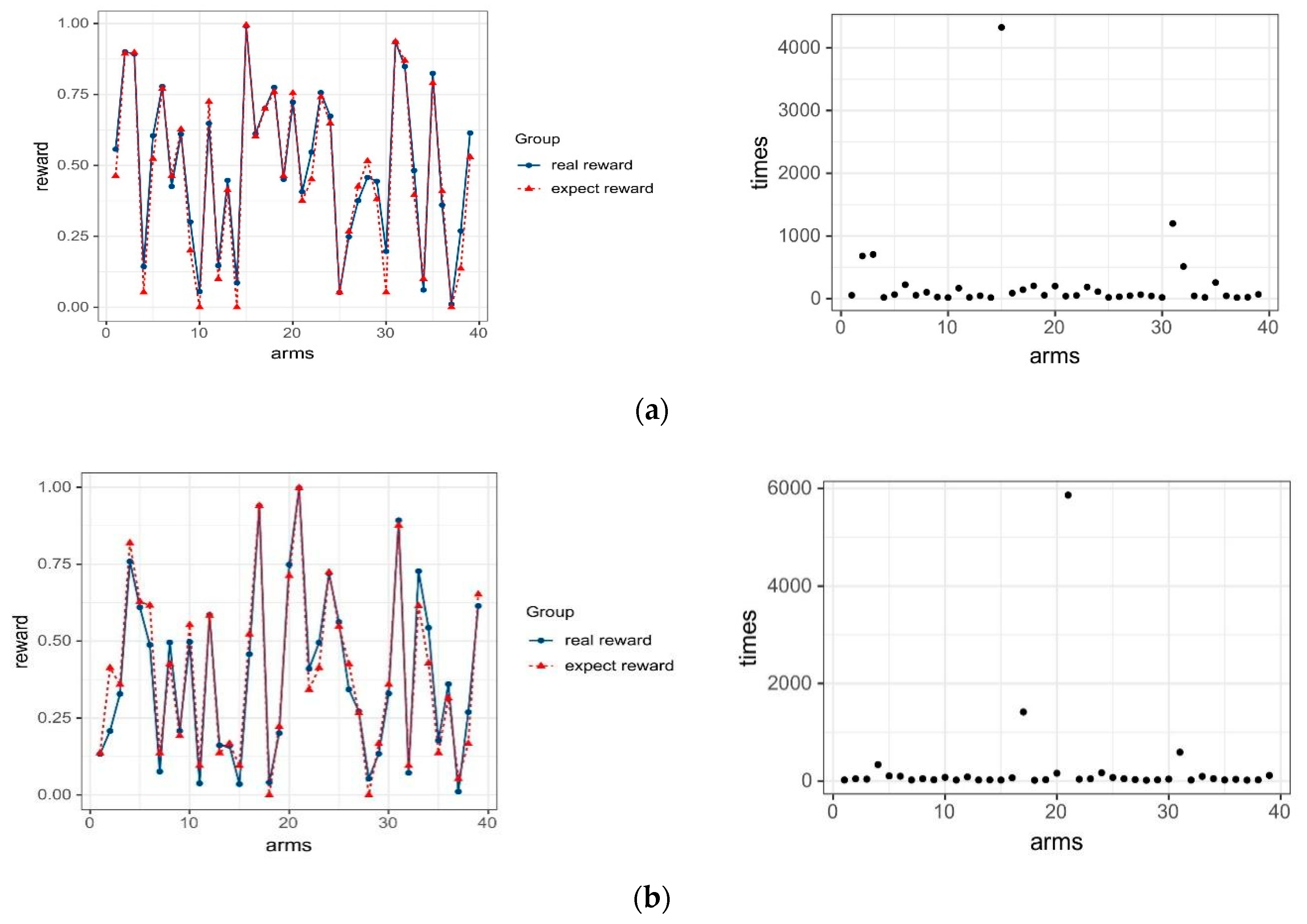
Figure 6 shows the situation of arm selection when a leakage occurs in the 15th and 21st pipes, respectively. In this case, the pipe with the largest UCB value has the maximum likelihood of being selected, followed by the pipe with the second-largest average UCB value. It validates the fact that LinUCB selects the pipe with the highest upper confidence bound. Additionally, it shows that the algorithm is correct and feasible.
4.3.3. Parametric Analysis
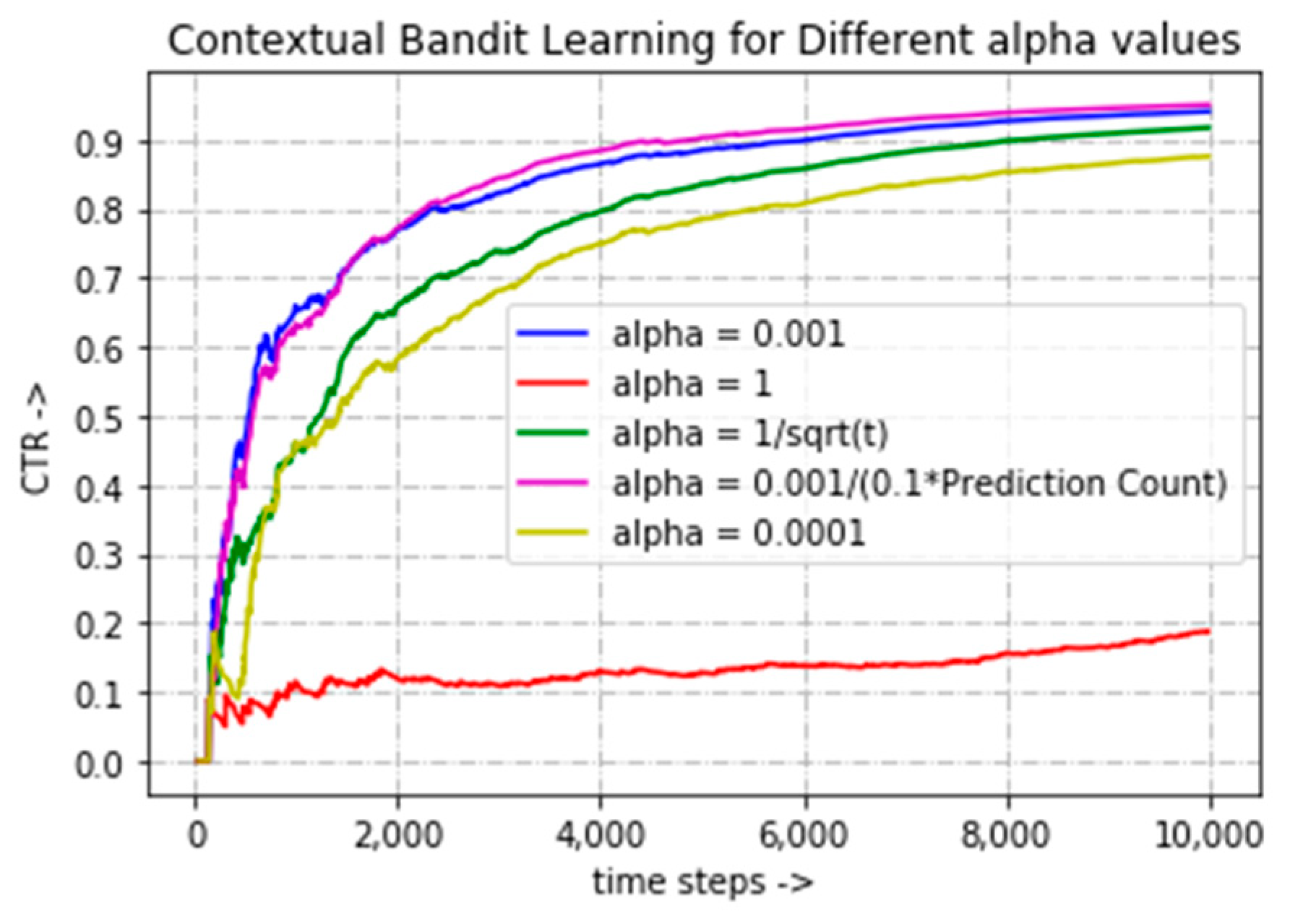
The explore–exploit mechanism in the algorithm is balanced by tuning the value of . Several different mechanisms are used to identify which value works the best. The values are taken as 1, 0.001, 0.0001, , and 0.001/(correct-selections/10), respectively. A comparative analysis of the various values shows how accuracy of the algorithm varies based on different values in Figure 7.
As is evident from the plots, the best CTR value is achieved with as “0.001/(number of correct selections/10)”, when the CTR value is 0.95. Subsequently, the CTR values are 0.94, 0.87, 0.91, and 0.20 for values of 0.001, 0.0001, and 1, respectively.
When the value is 1, we observe that the selected counts are almost the same for all arms due to the minimal number of exploitations, thus giving it a very poor CTR value of 0.2. A significant improvement in the results can be seen when changing the value of as a function of the square root of time step. This is mainly because the agent is regulating the degree of exploration and exploits the most out of the trained algorithm as the time passes.
A better result is obtained when using an value of 0.001. The reason for this is that in this case we are limiting the exploration to a very small value and exploiting the most. This assures a positive outcome for the experiment.
In order to improve the CTR and achieve better results on this dataset, we assigned = 0.001/(correct-selections/10) and obtained the best result so far. This increased the exploitation, particularly for the arms which gave us better results, and increased the exploration of the arms which have not been the best selections so far. This approach raised the CTR value of the LinUCB algorithm even further to 0.9508, which has been the best CTR rate of all the α values experimented with.
Moreover, it is apparent from the experimentation that the choice of is very important as it governs the exploitation versus exploration tradeoff and can drastically improve the results, if selected wisely.
5. Conclusions
In this paper, a new leakage fault detection method based on Contextual Bandit is proposed. The entire experimental results show that the LinUCB algorithm is helpful to solve the challenge of context-independence and construct an effective pipe selection model for leakage faults.
Our method has three major advantages, including a high accuracy of 95.08%, low investment and online real-time detection capabilities. As for the low-investment problem, our method does not require additional sensors and installation of other equipment, and the current existing sensors from substations and end-users are enough to obtain data. As for the online learning and real-time detection problem, the SCADA system or IBMS system can obtain real-time data online, which can provide a software basis for rapid fault detection. At the same time, LinUCB is also an online learning algorithm. Therefore, the LinUCB algorithm just needs to collect the sensor data in real time to train an agent, which can be used to identify the right leakage pipe. However, it is different from the traditional online learning method (such as Follow the Regularized Leader (ftrl), OpenDayLight (ODL), etc.). Two main differences are as follows: (1) traditional methods try to construct a unified model for the entire scenario, while each pipe in LinUCB is a separate model. (2) Traditional online learning methods use a greedy strategy for making decisions based on the learned knowledge without exploration (but greedy strategies are often not optimal). However, on the other hand, LinUCB has a more complete exploitation and exploration mechanism, and focuses on long-term cumulative rewards, which is much more appropriate for reflecting the optimal policy.
Since DHNs are closed recurrent networks, the amount of make-up water can be an indicator to identify if a leakage occurs in the network. The delayed alarm triggering algorithm is used to trigger an alarm when a malfunction occurs and reduce the measuring errors and the interference of noise at the same time [31]. As the uptime of the DHS is much longer than the downtime, real leakage data are relatively rare. Therefore, the established model is used to simulate and obtain data for all possible leakage faults. When the leakage signal is sent, the change rate vectors from the installed sensors are input into the trained model, which can quickly output the leaking pipe label. The experimental results show that the existing number of sensors can obtain enough data to ensure the LFD model achieves an excellent detection performance, and the detection accuracy can reach 95.08%. It also shows that this method can accurately and effectively detect leaking pipes, allow operators to evaluate system performance, support troubleshooting decision mechanisms, and provide assistance in the arrangement of maintenance [32]. At the same time, we think that our method is also applicable to the leakage fault detection of air conditioning water systems.
Although our method can achieve a fairly high accuracy, it relies heavily on accurate data and suitable pre-processing. Therefore, combining the sensor fault detection method and our method can perhaps increase the robustness of FDD. In addition, based on the investigation of single agent, future work will consider using a multi-agent to detect multi-point leakage faults. Moreover, the application of reinforcement learning in fault detection and diagnosis is our research plan in the future.
Author Contributions
Conceptualization, Y.S.; Data curation, Y.S.; Formal analysis, Y.S.; Funding acquisition, J.C.; Investigation, H.W., Y.W. and Y.L.; Methodology, Y.S. and Q.F.; Project administration, J.C., H.W., Y.W. and Y.L.; Software, Y.S.; Supervision, J.C., Q.F. and Y.L.; Validation, Y.S.; Writing—original draft, Y.S.; Writing—review & editing, Q.F. All authors have read and agreed to the published version of the manuscript.
Funding
The research was funded by the National Key Research and Development Program of China, grant number 2020YFC2006602, the National Natural Science Foundation of China, grant number 62072324, 61876217, 61876121, 61772357, and the Key Research and Development Program of Jiangsu Province, grant number BE2020026.
Conflicts of Interest
The authors declare no conflict of interest.
References
- Wang, J.; Cao, S.-J.; Yu, C.W. Development trend and challenges of sustainable urban design in the digital age. Indoor Built Environ. 2021, 30, 3–6. [Google Scholar] [CrossRef]
- Hering, D.; Cansev, M.E.; Tamassia, E.; Xhonneux, A.; Müller, D. Temperature control of a low-temperature district heating network with Model Predictive Control and Mixed-Integer Quadratically Constrained Programming. Energy 2021, 224, 120140. [Google Scholar] [CrossRef]
- Hussam, J.; Richard, M. Heat pipe based thermal management systems for energy-efficient data centres. Energy 2014, 77, 265–270. [Google Scholar] [CrossRef] [Green Version]
- Bai, L.; Liu, H.; Yu, C.W.; Yang, Z. Optimal diameter of district heating pipe network based on the hybrid operation of distributed variable speed pumps and regulating valves. Indoor Built Environ. 2021. [Google Scholar] [CrossRef]
- Liu, G.; Zhou, X.; Yan, J.; Yan, G. A temperature and time-sharing dynamic control approach for space heating of buildings in district heating system. Energy 2021, 221, 119835. [Google Scholar] [CrossRef]
- Li, H.; Long, E.; Zhang, Y.; Yang, H. Operation strategy of cross-season solar heat storage heating system in an alpine high-altitude area. Indoor Built Environ. 2020, 29, 1249–1259. [Google Scholar] [CrossRef]
- Yan, K.; Chong, A.; Mo, Y. Generative adversarial network for fault detection diagnosis of chillers. Build. Environ. 2020, 172, 106698. [Google Scholar] [CrossRef]
- Zhou, S.; O’Neill, Z.; O’Neill, C. A review of leakage detection methods for district heating networks. Appl. Therm. Eng. 2018, 137, 567–574. [Google Scholar] [CrossRef]
- Zhao, Y.; Zhuang, X.; Min, S. A new method of leak location for the natural gas pipeline based on wavelet analysis. Energy 2010, 35, 3814–3820. [Google Scholar] [CrossRef]
- Jia, Z.; Liang, R.; Li, H. Pipeline Leak Localization Based on FBG Hoop Strain Sensors Combined with BP Neural Network. Appl. Sci. 2018, 8, 146. [Google Scholar] [CrossRef] [Green Version]
- Xue, P.; Jiang, Y.; Zhou, Z. Machine learning-based leakage fault detection for district heating networks. Energy Build. 2020, 223, 110161. [Google Scholar] [CrossRef]
- Lei, C. Research on Leakage Fault Diagnosis of Heating Pipeline Network. Harbin Institute of Technology: Harbin, China, 2010. [Google Scholar]
- Morteza, Z.; Mehdi, S.; Karim, S. Pipeline leakage detection and isolation: An integrated approach of statistical and wavelet feature extraction with multi-layer perceptron neural network (MLPNN). J. Loss Prev. Process. Ind. 2016, 43, 479–487. [Google Scholar] [CrossRef]
- Berg, A.; Ahlberg, J.; Felsberg, M. Enhanced analysis of thermographic images for monitoring of district heat pipe networks. Pattern Recognition Letters. 2016, 83, 215–223. [Google Scholar] [CrossRef] [Green Version]
- Wang, J.; Hou, J.; Chen, J.; Fu, Q.; Huang, G. Data mining approach for improving the optimal control of HVAC systems: An event-driven strategy. J. Build. Eng. 2021, 39, 102246. [Google Scholar] [CrossRef]
- Martin, D.M.; Johnson, F.A. A Multiarmed Bandit Approach to Adaptive Water Quality Management. Integr. Environ. Assess Manag. 2020, 16, 841–852. [Google Scholar] [CrossRef]
- Gittins, J.C. Bandit Processes and Dynamic Allocation Indices. J. R. Stat. Soc. Ser. B Stat. Methodol. 1979, 41, 148–164. [Google Scholar] [CrossRef] [Green Version]
- Xue, P.; Jiang, Y.; Zhou, Z. Data for: Machine Learning-Based Leakage Fault Detection for District Heating Networks; Harbin Institute of Technology: Harbin, China, 2020. [Google Scholar] [CrossRef]
- Savchenko, A.V.; Milov, V.R. Decision Support in Intelligent Maintenance-planning Systems Based on Contextual Multi-armed Bandit Algorithm. Procedia Computer Science. 2017, 103, 316–323. [Google Scholar] [CrossRef]
- Sutton, R.; Barto, A. Reinforcement Learning: An Introduction, 2nd ed.; The MIT Press: Cambridge, MA, USA, 1992. [Google Scholar]
- Auer, P.; Cesa-Bianchi, N.; Fischer, P. Finite-time analysis of the multiarmed bandit problem. Mach. Learn. 2002, 47, 235–256. [Google Scholar] [CrossRef]
- Huang, K.H.; Lin, H.T. Linear Upper Confidence Bound Algorithm for Contextual Bandit Problem with Piled Rewards. In Proceedings of the Pacific-Asia Conference on Knowledge Discovery and Data Mining, Delhi, India, 11–14 May 2021; Springer: Cham, Swizterland, 2016; Volume 9652, pp. 143–155. [Google Scholar] [CrossRef]
- BI, W.; Guo, L. Product Pricing Algorithm Based on Multi-armed Bandit. Comput. Eng. Appl. 2021, 57, 224–231. [Google Scholar]
- Mark, A.M. Reinforcement Learning: MDP Applied to Autonomous Navigation. Mach. Learn. Appl. Int. J. 2017, 4, 1–10. [Google Scholar] [CrossRef]
- Kim, J.; Frank, S.; Braun, J.E.; Goldwasser, D. Representing Small Commercial Building Faults in EnergyPlus, Part I: Model Development. Buildings 2019, 9, 233. [Google Scholar] [CrossRef] [Green Version]
- Kim, J.; Frank, S.; Im, P.; Braun, J.E.; Goldwasser, D.; Leach, M. Representing Small Commercial Building Faults in EnergyPlus, Part II: Model Validation. Buildings 2019, 9, 239. [Google Scholar] [CrossRef] [Green Version]
- Barone, G.; Buonomano, A.; Forzano, C.; Palombo, A. A novel dynamic simulation model for the thermo-economic analysis and optimisation of district heating systems. Energy Convers. Manag. 2020, 220, 113052. [Google Scholar] [CrossRef]
- Lei, C.; Zou, P. Application of neural network in heating network leakage fault diagnosis. J. Southeast Univ. Engl. Ed. 2010, 26, 173–176. [Google Scholar]
- Zhou, Z. Machine Learning; Tsinghua University Press: Beijing, China, 2016. [Google Scholar]
- Walsh, T.J.; Szita, I.; Diuk, C. Exploring compact reinforcement-learning representations with linear regression. In Proceedings of the Twenty-Fifth Conference on Uncertainty in Artificial Intelligence, Montreal, QC, Canada, 9 May 2012. [Google Scholar]
- Li, L.; Chu, W.; John, L.; Robert, E.S. A Contextual-Bandit Approach to Personalized News Article Recommendation; Association for Computing Machinery: New York, NY, USA, 2010; pp. 661–670. [Google Scholar] [CrossRef] [Green Version]
- Xue, P.; Zhou, Z.; Fang, X. Fault detection and operation optimization in district heating substations based on data mining techniques. Appl. Energy 2017, 205, 926–940. [Google Scholar] [CrossRef]
Figure 1.
A District Heating System (DHS).

Figure 2.
The relationship between state and action in different bandit algorithms.

Figure 3.
Flowchart of leakage fault detection for Contextual Bandit.

Figure 4.
Supply water network in a DHS (diagram).

Figure 5.
Comparison of four arm selection methods.

Figure 6.
Left: reward prediction and right: arm selection when leakages occur in the (a) 15th and (b) 21st pipes. (On the left figure, the Y axis shows the reward for each pipe, and the X axis shows the number of pipes (i.e., the arm to be selected). The Y axis in the right figure represents the number of choices made by the agent, and the X axis represents the pipe to be selected).

Figure 7.
CTR values for different α values.


Table 1.
Heat source and user flow design information.
| User-ID | Pipe Name | Mass | User-ID | Pipe Name | Mass |
|---|---|---|---|---|---|
| U0 | n1 | 2196.4 | U8 | n30 | 458.9 |
| U1 | n23 | 75.7 | U9 | n31 | 118.7 |
| U2 | n24 | 172.7 | U10 | n32 | 49.6 |
| U3 | n25 | 214.4 | U11 | n33 | 183.2 |
| U4 | n26 | 116.2 | U12 | n34 | 187.4 |
| U5 | n27 | 148.3 | U13 | n35 | 67.2 |
| U6 | n28 | 25.3 | U14 | n36 | 143.4 |
| U7 | n29 | 16.9 | U15 | n37 | 218.5 |
Table 2.
Pipe network design information and data quantity.
| Parameter | Number |
|---|---|
| Number of main pipes (supply water and return water) | 78 |
| Number of flow sensors | 16 |
| Number of pressure sensors | 31 |
| Number of data collected per pipeline leakage | 100–400 |
| Number of training sets | 10,609 |
| Number of test sets | 4506 |
Publisher’s Note: MDPI stays neutral with regard to jurisdictional claims in published maps and institutional affiliations. |
© 2021 by the authors. Licensee MDPI, Basel, Switzerland. This article is an open access article distributed under the terms and conditions of the Creative Commons Attribution (CC BY) license (https://creativecommons.org/licenses/by/4.0/).
Share and Cite
MDPI and ACS Style
Shen, Y.; Chen, J.; Fu, Q.; Wu, H.; Wang, Y.; Lu, Y. Detection of District Heating Pipe Network Leakage Fault Using UCB Arm Selection Method. Buildings 2021, 11, 275. https://0-doi-org.brum.beds.ac.uk/10.3390/buildings11070275
AMA Style
Shen Y, Chen J, Fu Q, Wu H, Wang Y, Lu Y. Detection of District Heating Pipe Network Leakage Fault Using UCB Arm Selection Method. Buildings. 2021; 11(7):275. https://0-doi-org.brum.beds.ac.uk/10.3390/buildings11070275
Chicago/Turabian StyleShen, Yachen, Jianping Chen, Qiming Fu, Hongjie Wu, Yunzhe Wang, and You Lu. 2021. "Detection of District Heating Pipe Network Leakage Fault Using UCB Arm Selection Method" Buildings 11, no. 7: 275. https://0-doi-org.brum.beds.ac.uk/10.3390/buildings11070275
Note that from the first issue of 2016, this journal uses article numbers instead of page numbers. See further details here.