Reliability Analysis of Reinforced Concrete Frame by Finite Element Method with Implicit Limit State Functions


1
Faculty of Civil Engineering and Architecture Osijek, University of Osijek, 3 Vladimir Prelog Street, HR–31 000 Osijek, Croatia
2
TRINAS Projekt Ltd., 14 Dubrovačka Street, HR–31 000 Osijek, Croatia
*
Author to whom correspondence should be addressed.
Buildings 2019, 9(5), 119; https://0-doi-org.brum.beds.ac.uk/10.3390/buildings9050119
Submission received: 8 February 2019
/
Revised: 29 April 2019
/
Accepted: 5 May 2019
/
Published: 10 May 2019
Abstract
:Since the prediction of the seismic response of structures is highly uncertain, the need for the probabilistic approach is clear, especially for the estimation of critical seismic response parameters. Considering the uncertainties present in the material and geometric form of reinforced concrete (RC) structures, reliability analyses using the Finite Element Method (FEM) were performed in the context of Performance-Based Earthquake Engineering (PBEE). This study presented and compared the possibilities of nonlinear modelling of the reinforced concrete (RC) planar frame and its reliability analysis using different numerical methods, Mean-Value First-Order Second-Moment (MVFOSM), First-Order Reliability Method (FORM), Second-Order Reliability Method (SORM) and Monte Carlo simulation (MCS). The calibrated numerical models used were based on the previous experimental test of a planar RC frame subjected to cyclic horizontal load. Numerical models were upgraded by random variable (RV) parameters for reliability analysis purposes and, using implicit limit state function (LSF), pushover analyses were performed by controlling the horizontal inter-storey drift ratio (IDR). Reliability results were found to be sensitive to the reliability analysis method. The results of reliability analysis reveal that, in a nonlinear region, after exceeding the yield strength of the longitudinal reinforcement, the cross-sectional geometry parameters were of greater importance compared to the parameters of the material characteristics. The results also show that epistemic (knowledge-based) uncertainties significantly affected dispersion and on the median estimate parameter response. The MCS sampling method is recommended, but the First-Order Reliability Method (FORM) applied on a response model can be used with good accuracy. Reliability analysis using the FEM proved to be suitable for the direct implementation of geometric and material nonlinearities to cover epistemic (knowledge-based) uncertainties.
1. Introduction
Structural design aims to achieve structures that satisfy safety criteria, serviceability and durability under specified service conditions. Since uncertainty is an inherent characteristic that cannot be avoided in engineering design, incorporating uncertainties in engineering design is required [1]. Reliability analysis offers a well-established theoretical framework for considering uncertainties in the engineering decision scheme. We can define reliability as the probability that a structure or system can perform a required function (or limit state function, LSF) under specified service conditions during a given period and stated conditions [2]. Conversely, the failure probability, (or probability of failure) is the probability that a structure does not perform satisfactorily within a given period and stated adverse conditions [3].
In the context of seismic risk analysis, the probability of exceeding the given LSF, obtained from the reliability analysis, is integrated with the seismic risk of the locality. The related term used in conjunction with seismic reliability analysis and structural risk is a fragility analysis. The fragility analysis is aimed at finding the probability of a particular structural failure for different levels of intensity measures (IM) such as PGA (peak ground acceleration) or (, 5%) (5%-damped elastic first period spectral acceleration), and analysis is closer to the true estimation of structural seismic risk. Despite these fine distinctions, seismic risk, reliability, safety, and structural fragility analysis are used in various ways to denote the seismic probability of structural failure, so that the failure is defined by different structural limit states conditions [4].
The most important aspect of the structural reliability analysis is the consideration of uncertainties that make a structure vulnerable to failure for a pre-defined limit state condition. The accuracy of the reliability analysis depends on how exactly all the uncertainties are considered during analysis. First, the challenge is to identify all the sources of uncertainties; therefore, crucial uncertainties must be identified. Second, the techniques of explicit or implicit modelling are difficult to implement, therefore a certain degree of uncertainty is associated with the modelling method, with some necessary simplifications. Finally, the analytical formulation of the limit state equations and integrating the probability density function (PDF) in this domain is complex and results in various approximations. Consequently, there are different degrees of simplification in the reliability analysis leading to various reliability analysis methods, as explained below [5,6].
Considering the foregoing, the bearing capacity of the structure or element can be obtained in many ways, being the most simple and direct to use an explicit design equation, when the LSF can be expressed as an explicit form or simple analytical form in terms of the basic variables x, which characterise the structural behaviour, relating the many variables, defined by probabilistic distributions. If an explicit function capable of defining the behaviour of the structure is not available, it is possible to use the FEM with implicit LSF to compute the behaviour of the structure. Such implicit LSF are encountered when the structural systems are complicated and numerical analysis such as FEM must be adopted for the structural response prediction.
We can simplify the safety assessment procedure with implicit functions, by getting an alternative explicit LSF that allows a significant decrease in the response calculation time. We can obtain this function through the Response Surface Method (RSM) by fitting a surface to various realisations, for a set of variables, based on an MCS using an implicit LSF provided by the FEM [7,8]. In addition to all the well-established postulates of individual reliability methods, one of the hypotheses of this study is that, even when using the FEM, the least numerical model settings can have a relatively significant impact on the reliability analysis results. These settings relate to the type of element, the plastic hinge length, the number of integration points along the element, numerical integration options for the force-based beam–column element, geometric transformation type, etc.
The described procedures in this study are compatible with the implementation of the model in the PEER PBEE framework (Pacific Earthquake Engineering Research Performance-Based Earthquake Engineering) [9,10], which besides structural responses takes into account the consequent functions and interaction with the Performance Assessment Calculation Tool (PACT P-58) [11]. Flexible feature of this approach is two-way communication with Python and MATLAB, which is important for the application of sophisticated sampling techniques.
This paper presents the numerical calibration of the experimental RC frame model, which was later upgraded for reliability analysis purposes. The methods of reliability analysis of MVFOSM, FORM, SORM and MCS were used, after which the basic results and conclusions were presented. All numerical analyses presented in this paper were carried out by combining OpenSees and MATLAB with customisable algorithms.
Reliability Analysis Methods
The mean value first-order second moment (MVFOSM) method is the simplest and least expensive reliability method. This method estimates the mean and variance of the LSF based on the first-order Taylor series approximation of the LSF and its derivatives at the mean values of the random input variables. Then, these two statistics (mean and variance) of the LSF are used to calculate the reliability index, . Approximations of the mean and variance of LSF are sufficiently accurate only when the LSF is nearly linear and the input random variables are approximately Gaussian. In other situations, MVFOSM method does not guarantee accuracy.
To overcome these significant limitations of MVFOSM method by approximating the LSF at the optimal point, called Design Point or Most Probable Point (MPP), in uncorrelated standard normal space (U-space) rather than in the origin actual variables space (X-space), which may be correlated and non-normal. This kind of method contains two Design Point-Based Methods approaches, the first-order and second-order reliability methods (FORM and SORM, respectively). In the first-order reliability method (FORM), we linearise the LSF in U-space by the first-order Taylor expansion at the Design Point. The first-order approximation in FORM works well because the neighbourhood of the design point has a dominant contribution to the failure probability. However, if the limit state function (or surface) is strongly non-flat or the optimisation problem has multiple local or global solutions, the first-order approximation may not work well. The SORM is driven by improving the capability of the approximation when the limit state surface is non-flat.
The second-order reliability method (SORM) approximates the LSF by the second-order Taylor expansion at the design point. Since the LSF is approximated by second-order Taylor expansion, the limit state surface is approximated by a paraboloid in SORM rather than by a linearised plane in FORM. To obtain the second-order approximation of the failure probability, the curvatures of the paraboloid need to be evaluated.
In many practical problems, the LSF may not be known explicitly. Instead, it may be known only implicitly, through a procedure such as a FEM, and often is expensive to evaluate, especially with a very fine degree of numerical modelling and many degrees of freedom. This means that the safe domain can be defined only through a point-by-point discovery such as through repeated numerical analysis with different input values, i.e., sampling methods, such as the Monte Carlo simulation (MCS). In these conditions, it is apparent that the FORM and SORM and related methods, which require a closed and preferably differentiable form for the LSF, are not immediately applicable. This has led to the development of the Response Surface Method (RSM) for reliability analysis. In RSM, the implicit LSF is replaced by an artificially constructed function , generally a polynomial, around the design point [1,2,3].
2. Experimental Model
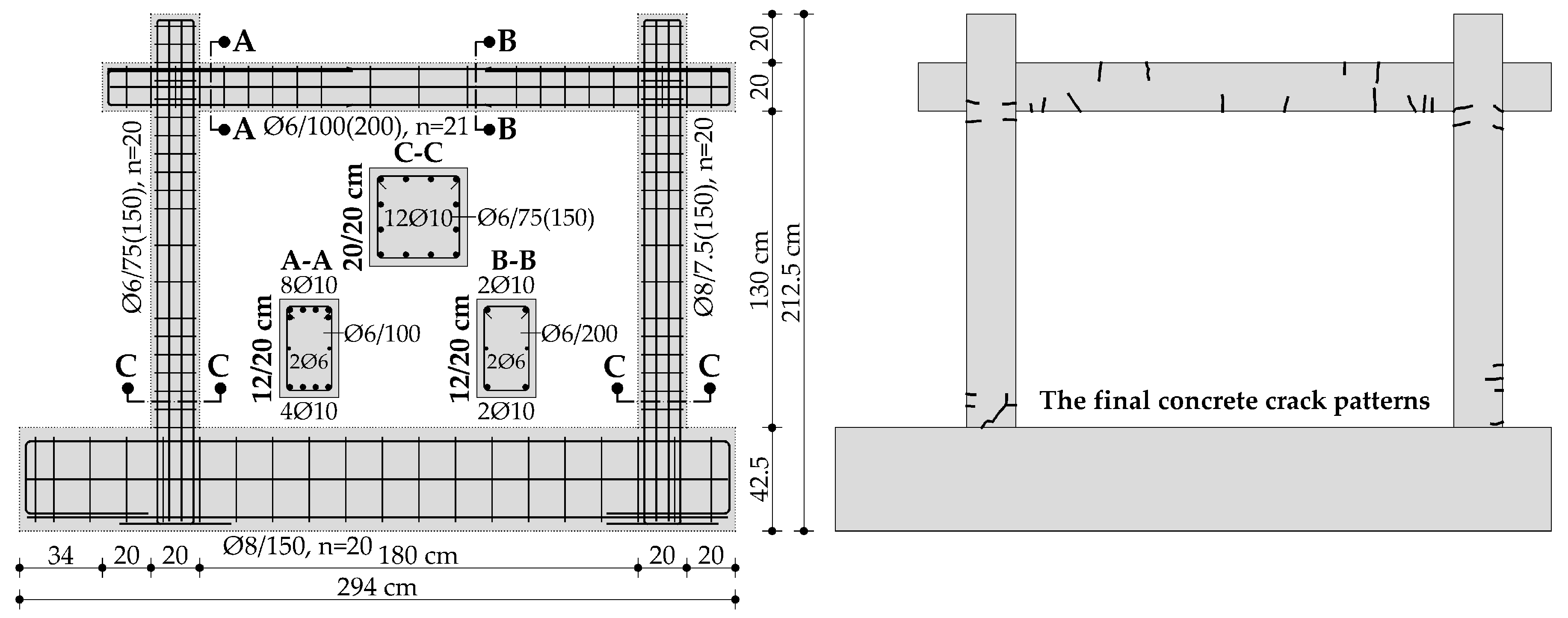
In accordance with the prototype of a typical mid-rise building, central bay RC frame from the ground floor was chosen and constructed at a scale of 1:2.5, which makes an aspect ratio of 1.4 [4,12,13]. Geometry, cross sections, and the amount of main longitudinal and transverse reinforcement is shown in Figure 1. The prototype of a typical building [14], from which the central frame on the scale was separated, was designed in accordance to the relevant codes [15,16], for ductility class DCM, required design concrete grade C30/37 and reinforcement B500B. The actual mechanical properties, modulus of elasticity, yielding strength, and ultimate strengths were determined in accordance with the applicable norms. After the frames were made and concrete samples were tested, the average compressive strength of the concrete cubes was 50 MPa, while the yielding and ultimate tensile strength, and the modulus of elasticity of the reinforcement were 550, 650 and 210,000 MPa respectively. All these parameters of material characteristics were determined by standardised compressive and tensile tests, whose values were rounded off from a series of nine repeated tests. The model was cyclically tested in a horizontal direction, with a constant total vertical force in columns of 730 kN, i.e., 365 kN per column, to ensure an axial load ratio of 18% in each column, as defined by the design (9 MPa of the axial stress relative to the gross cross-section of the column). During testing, the horizontal force was controlled, i.e., beam level displacement up to 1.0% of inter-storey drift ratio (IDR) or 14 mm, by repeating each cycle twice, resulting in damage to the ends of the columns and the beam by crushing the concrete and reaching the yield strength of individual longitudinal reinforcement.
Figure 2 shows the hysteresis curve as a basic view of the system’s behaviour, with insight into the secant stiffness (K), bearing capacity and ductility of the system and the trend of component stiffness degradation. To evaluate analytically the initial elastic stiffness of the system for the purpose of calibrating the numerical model, we can use the equation for the upper lateral stiffness limit for the shear-type frame: , where is the elastic modulus of the columns, is the second moment of the column cross-sectional area and L is the length of the columns. The mean modulus of elasticity of concrete is = 36,050 MPa (plain concrete modulus). Considering the amount of longitudinal reinforcement ( mm), the columns elasticity modulus increased by 11%, i.e., = 40,100 MPa (including cross-sectional reinforcement). Therefore, the analytical initial lateral stiffness was 58.4 kN/mm, while experimentally determined (based on the trilinear backbone curve) was 60 kN/mm. The results of the experiments and the observation of the model during the test phases of damage development are described, as well as the failure mechanisms and damage levels. When describing the behaviour of such models, it is necessary to evaluate the stiffness, strength and deformation properties of individual components to numerically model the same effects and expand the analysis, such as sensitivity or reliability analysis.
The phases of damage development are described according to the above criteria starting with the formation of the first cracks due to bending at the base of the columns, at a horizontal drift of 0.05% and a horizontal force of 30 kN. The first crack on the beam was developed at a 0.76% drift while at the 0.86% drift the concrete cover started spalling at the base of the columns. Once the horizontal force of 170 kN was reached, the frame was no longer capable of taking a further gain of force while the horizontal drift increased. The specimen was not tested until the collapse but up to the targeted drift of 1.0% to preserve the specimen for further testing. The distribution and the type of cracks showed a clear flexural behaviour, with no shear failures.
The definition of the trilinear backbone curve (i.e., bearing capacity curve), which represents the three different areas of behaviour, is based on the mean value of the bearing capacity of the positive and negative horizontal direction, as shown in Figure 3. When defining the trilinear backbone curve, the formation moment of the first significant crack was considered (1), as well as the continuation of cracks development up to the level of the global model yielding, i.e., temporary lack of bearing capacity (2) and the targeted drift (3). Such load bearing envelope is suitable for describing behaviour in numerical modelling, using the SDOF model, whereby such a backbone can be attributed to rotational or translational spring as translational or rotational stiffness parameters with corresponding hysteresis behaviour. The characteristic points of the trilinear backbone curve and the stiffness curve were: %, kN, and kN/mm.
3. Numerical Model
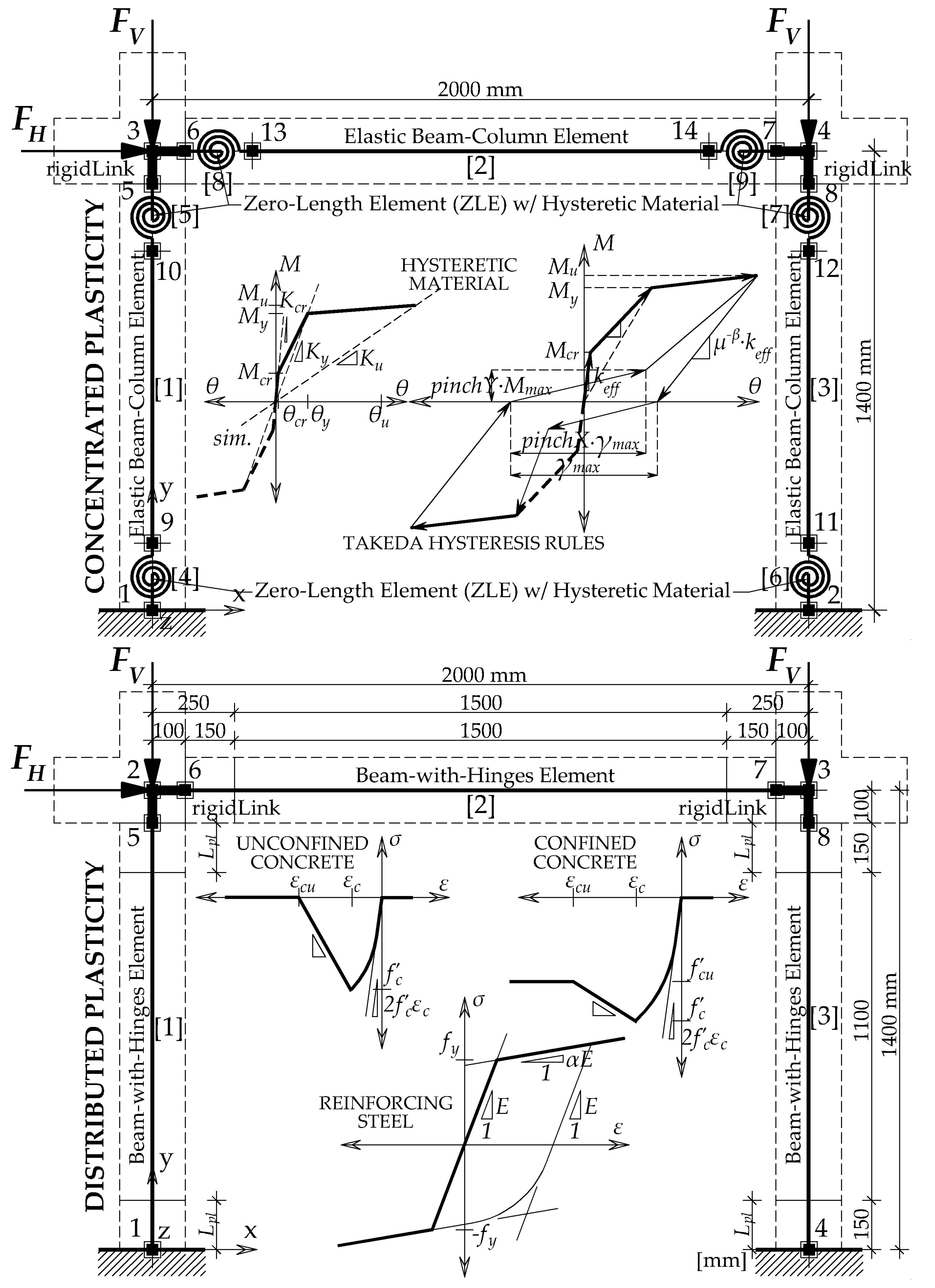
The numerical model is constructed in two ways by the OpenSees (Figure 4) to construct as simpler a model as possible to adequately describe the frame behaviour in relation to experimental testing.
3.1. Concentrated (Lumped) Plasticity Model (CP)
In the first part of modelling hysteresis response, a well-known approach to the theoretical semi-empirical model of concentrated plasticity (CP) was used, with hysteresis rules for RC elements according to Takeda [17], for easier and robust control of hysteresis behaviour. At the ends of columns and beams, the characteristics of the parameters according to the Takeda hysteresis rule were associated. Boundary conditions at the bottom of the columns were considered as absolutely fixed, as were the panel-zone of the beam–column joints (rigidLink and equalDOF).
The ultimate bending moment was adopted as a moment at the fracture of the first major longitudinal reinforcement, while the yielding moment was defined as a bending moment corresponding to the first longitudinal reinforcement yielding of each element individually. Cracking moment and rotation corresponded to the initial cracking of concrete, whereby the tensile strength of the concrete was taken into consideration as 3.5 MPa according to the Eurocode 2 EN1992-1:2004 [15], based on the compressive strength of the concrete. The plastic hinge length calculation was performed according to Paulay and Priestley [18] whose length was rounded to 20 cm. Cross-sectional analyses were also carried out to determine the relationship between the bending moments and section curvatures of each element individually (moment–curvature, M–) to further define the bearing capacity of individual elements as the moment–rotation relationship, M–.
The Hysteretic material used for simulating hysteresis behaviour (containing additional pinch, damage, and beta parameters) was attributed to the rotational springs by a zeroLength element, is a Hysteretic material used. The elements between the rotational springs were linearly elastic (elasticBeamColumn) since all plasticity was retained at the very ends of the elements (the greatest internal forces) with the corotational transformation (P– effects) considered in the model [19,20,21,22]. The numerical model considers the cracked elements, as recommended by [16] [EN 1998-1/4.3.1(6)]. The elastic flexural stiffness properties were taken to be equal to one-half of the corresponding stiffness of the uncracked elements [16] [EN 1998-1/4.3.1(7)], i.e., the moment of inertia of the uncracked section was multiplied by a factor 0.5. This value was subsequently verified by cross-sectional analysis (moment–curvature relationship, M–). In this way, hairy cracks (<0.5 mm) were compensated on the beams. Other details in the configuration of this model can be found in [4].
Figure 5 compares the numerical hysteresis curve with the experimental hysteresis response (left) and numerical pushover curve with the experimental mean backbone curve (right), both for the CP model. The model shows enough compatibility for this short study in terms of bearing capacity, ductility, or nonlinear behaviour.
It should be noted that both CP and DP numerical models are, by definition, suitable for reliability analysis. For this study, the DP model was chosen only because of engineering comprehension and the easier understanding of RVs and their associated coefficients of variation (COV). The nonlinearities in the CP model are defined based on the moment–rotation relationship (M–), which may be less understandable for practitioners, especially due to the lack of knowledge about the dispersion of these parameters at the yielding limit and ultimate bearing capacity. The nonlinearities in the DP model are defined by fibre sections, which have implemented uniaxial material behaviour parameters, based on which RVs are defined. All variables in the DP model are engineer understandable and dispersion of these parameters is well documented in the literature.
3.2. Distributed Plasticity Model (DP)
The previous numerical model was modified in such a way that, instead of rotational springs (Concentrated Plasticity, CP), fibre cross sections were implemented in a model with uniaxial nonlinear behaviour of constitutive materials (Distributed Plasticity, DP), as shown in Figure 6. The reason for this modification lies in the method of defining (assigning) RV parameters. To facilitate the understanding and control of defining the RV parameters, DP defines all RV parameters that are engineer-understandable and whose parameters can be relatively easily experimentally determined. These RVs are material and geometric characteristics in relation to the dominant empirical moment–rotation relationships in the CP model.
BeamWithHinges element was used for modelling columns and beams, which considers force-based distributed plasticity over specified plastic hinge lengths near the element ends. Two-point Gauss–Lobatto integration rule was used over the hinge regions, where the bending moments were largest, which gave the desired level of element integration accuracy [23,24]. The basic uniaxial material models were attributed to fibre cross sections to keep the model as simple as possible, but also due to certain limitations in the OpenSees program’s sensitivity module at the time of the study. These uniaxial materials are Concrete01 (Kent–Scott–Park) for concrete and Steel01 (Bi-linear) for reinforcing steel. It should be emphasised that the initial modulus of elasticity of concrete directly depends on the peak strength and the associated deformation, expressed as . Fracture energy in compression for the Kent–Scott–Park concrete model can be expressed as . Additional introduced model parameters for the Kent–Scott–Park concrete model are elastic modulus, , strain corresponding to 20% of the compressive strength, . The parameter is the concrete fracture energy in compression (plain concrete crushing energy), which often serves for material regularisation and is the plastic hinge length, which acts as the characteristic length for the purpose of providing an objective response. The plastic hinge length was specified using an empirically validated relationship, such as the [18] equation for reinforced concrete members [kN, mm], where L is the length of the member and and are yield strength and diameter, respectively, of the longitudinal reinforcing bars. The advantage of this approach is that the plastic hinge length includes the effect of strain softening and localisation as determined by experiments. Finally, the plastic hinge length was adopted as 150 mm for columns and beam. Since the parameters and are directly related to the parameters and , they are not further considered as RVs, as defined below.
The confinement factor for columns and beams was adopted as a rounded value of 1.15, for a given cross-sectional configurations and transverse reinforcement spacing (which is closed at 135 degrees). Corotational geometric transformation was also applied in the DP model in order to consider the second-order effects [19,20,21,22]. The beam–column joints were considered rigid, as well as the base of the columns with a foundation. Detailed information on the parameters and settings for reliability analysis are given below.
4. Reliability Analysis
Based on the modified and updated numerical model, implementing the reliability analysis is presented. Professor Michael H. Scott (OSU, USA) and professor Terje Haukaas (UBC, Canada) contributed most to the OpenSees upgrade in terms of reliability analysis, whose publications are most significant in this research area [25,26,27]. From the aspect of the numerical capabilities of the program itself, the FEM constructed in OpenSees can be used to analyse the reliability on structural, elemental and cross-sectional levels, using static or dynamic (transient) analysis. This is significant since there is no limitation on the load types, integration methods, solution algorithms, geometric transformations or degrees of freedom (DOF). Consequently, structural performance can be expressed as a simple algebraic function of capacity minus demand (implicit LSF), as with most PBEE applications [28]. Therefore, the definition of the implicit LSF is reduced to the limitation of the resistance, internal forces, nodal displacement, or the deflection of the elements.
The calibrated numerical model shown was upgraded with defined RVs of normal (N) and log-normal (LN) distributions and defined parameters associated with RVs. It should be emphasised that the numerical model was adapted to the extent that its elements or sections were defined as fibre sections, therefore not defined by springs, whose characteristics were also derived from the fibre cross-sectional analysis. The reason for this was an easier understanding of RVs and its associated parameters. As RVs, we wanted to define the parameters of material characteristics, cross-sectional geometry, depth of the concrete cover, etc. compared to the parameters of the concentrated plasticity or the pair of moment–rotations (which is not a limit, but an intuitive approach has been adopted). The definition of RVs primarily refers to parameters of material properties of concrete and reinforcing steel, and then the geometrical characteristics of the cross section and the width and height of the RC frame. The mean values of all RVs were obtained from the experiments and calibrations, while their coefficients of variation (COV) were obtained partly from experimental material testing by comparing available literature (Table 1).
To present the possibilities of reliability analysis by FEM, a correlation between individual parameters or RVs was introduced. For example, a correlation introduced between the yielding strength and the modulus of elasticity of reinforcing steel as 60% correlation, as obtained from literature [25,29,30]. A complete correlation was found between the peak compressive strength of concrete for the concrete cover and core (i.e., unconfined and confined concrete section) and for the associated deformation, as 100% [25]. Thus, the importance of some RVs for the LSF could be ranked according to two parameters: and (Importance vectors). Thus, the importance vector does not consider the correlation between RVs, while the importance vector considers the defined correlation.
In Table 1, the symbols of the parameters show: the reinforcing steel yield strength (), the elasticity modulus of the reinforcing steel (), the compressive strength of the confined concrete core with corresponding deformation (, ), the compressive strength of the unconfined concrete with corresponding deformation (, ), the confined concrete crushing strength with corresponding deformation (, ), the unconfined concrete crushing strength with corresponding deformation (, ), the vertical load per column (), the length of the columns and beam (, ), the depth of the concrete cover for both columns and beams (), the cross section depth of the columns and beam (, ) and plastic hinge length for both columns and beam ().
The approach of the reliability analysis by the FEM has the advantage of reducing the uncertainties most present in the explicit definition of the LSF, the form of which is complicated, considering the geometric and material nonlinearity and the static indeterminacy of the system. To assess the reliability of horizontal loads, in the domain of earthquake engineering, it is enough to define the implicit LSF by limiting the Engineering Demand Parameter (EDP), which in the case of structure is any form of displacement, deformation or rotation as a good measure of demand (causing potential damage) [39,40]. Material and geometric nonlinear parameters, formulation of boundary conditions, static indeterminacy and a number of DOF are already defined within the numerical model, so the evaluation of RVs and the implicit LSF for the calculation of structural responses is easier regarding defining explicit LSF.
The following settings are defined for reliability analysis: Nataf transformation is a function which maps a random vector from x-space with a Gaussian copula to a random vector in u-space with standard Gaussian distribution, Implicit gradient estimation defines how to evaluate baseline variable gradients, iHLRF iterative solution scheme, i.e., optimisation algorithm (Hasofer–Lind–Rackwitz–Fiessler) defines how bearing capacity or resistance (R) and load effect (E) variables are standardised in new and variables (standard normal space), the Armijo rule defines the step size and sufficient descent condition to achieve the stabilisation of the FORM algorithm (sensitivity convergence), and the Search Step determines the maximum number of iterations to achieve convergence.
Figure 6 shows the pushover curve of a fibre-based numeric model regarding the cyclic response of the experiment. In the same figure, the IDR limit is defined for the ultimate LSF. In addition, the constant horizontal load value of 150 kN was adopted, which for this deterministic model is the amount of horizontal load at which the yielding strength is exceeded of reinforcing steel, after which the RC frame progressively loses its horizontal load bearing capacity. Thus, the limit state of the displacement is limited to 14 mm or 1.0% IDR the frame, as defined by the LSF (1). For all reliability analyses, MVFOSM, FORM, SORM and MCS, the static pushover analysis was used by controlling a horizontal load in 30 steps up to reaching the final 150 kN. Thus, the horizontal load was applied in steps of 5 kN, and the response of the structure in terms of the IDR was monitored. The primary equation of the implicit LSF is as follows (note that shows the horizontal displacement of the node #3):
The aim of all reliability analysis is to verify their comparability and applicability, thus, for Monte Carlo simulation (MCS), we expect the probability of for a reasonable number of simulations () close to FORM and SORM analyses. The SORM method improves the assessment given by FORM by including information about the curvature, approximating the nonlinear LSF (which is related to the second-order derivatives of the LSF with respect to the basic variables), while FORM approach approximates the LSF with a linear function. In addition to Monte Carlo sampling, another important sampling technique called Importance sampling needs to be mentioned, which improves the efficiency of Monte Carlo sampling by centring the sampling distribution near the failure domain. The point of minimum distance from the origin to the limit state surface, represents the worst combination of the probabilistic variables and is appropriately named the Design Point or the Most Probable Point. Importance sampling is efficient and requires fewer simulations than Monte Carlo sampling since the sampling distribution is centred on the Design Point, where failure realisations are frequently encountered. This technique, although available, is not covered by this study, but conventional MCS has been used.
5. Reliability Analyses Results
5.1. MVFOSM, FORM, and SORM Analyses
For different types of reliability analysis, it is interesting to compare the probability of exceeding the LSF. Table 2 and Table 3 show the rank list of RVs and their ranked importance vectors, obtained from the FORM analysis, according to the and vectors, respectively, by considering and not considering the correlation between the defined RVs for the given LSF .
Table 2 and Table 3 show the difference in the order of importance vectors with and without a defined correlation. The values of show the values of individual parameters for the same horizontal load of 150 kN reaching exactly the Design Point response, which is defined by the LSF and in this case was 14 mm or 1.0% of IDR. The pushover curves with the mean values of all parameters, and the design point values, are shown below for all MCS. The values of can also optimise the system in such a way that the iterative procedure monitors the mean value difference regarding design point values , thereby rationalising certain cross section dimensions, frame geometry or mechanical properties of the material (reliability-based design optimisation). It is important to emphasise that the list of parameters of RV, ranked by the importance vectors, is certainly sensitive to specific implicit LSF, i.e., the order of importance vectors does not apply to any other pre-defined LSF, which is visible from the Tornado Diagram Analysis (TDA). In addition, most design solutions will remain in the linear range of behaviour throughout their lifetime, where the optimisation of such linear systems would be even simpler, and there would be no significant between individual LSFs regarding the importance of some RVs if the structure behaves linearly.
Correlation affects not only the parameters to which it relates, but also all the parameters with which they interact within a numerical model. At the cross-sectional level, maximum compressive strength of the confined and unconfined concrete, and , the total height of the beam and columns cross section, and , the depth of the concrete cover for both columns and beams affecting the effective height of the cross sections, and yield strength of reinforcing steel, were the most sensitive parameters for the main LSF, considering the correlation between the parameters. Since the characteristics of reinforcing steel affect the behaviour of the confined concrete, the parameter became the most important parameter for the LSF . It is interesting that the first 8 of 17 parameters (Table 2 and Table 3) were equally important by considering and ignoring the parametric correlation, except parameter . The concrete crushing strengths ( and ) and deformations at the maximum concrete strengths ( and ) and the plastic hinge length () proved to be the least significant parameters for the main LSF. The focus of the parameters for the main LSF should be in Table 2, since most RVs were not statistically independent ().
The FORM analysis was completed with a total of 29 iterations using the HLRF procedure, evaluating a total of 60 approximations of g-functions. SORM analysis was also performed in two ways: by adopting the First Principal Curvature, SORM-FP, and applying Curvature Fitting by combining 10 curvatures for better approximation of the SORM-CF reliability index. The difference in the reliability index of and was only 0.127%, thus the probability of the limit state exceeds % or %. Furthermore, a comparison of the two additional LSF was added (10 mm and 6 mm of horizontal displacements) to compare the trend of declining reliability with respect to the reduction of the LSF. In Table 4, the reliability indexes for MVFOSM, FORM, SORM-FP and SORM-CF were compared for the 14 mm, 10 mm and 6 mm horizontal displacements as LSF. During these analyses, it was concluded that the ranks of important parameters based on and vectors were not the same for all three LSF, which is common for nonlinear systems since not all parameters affect equally the predominantly linear and nonlinear part of the model response. Based on these conclusions, a tornado diagram is constructed [32,41,42,43], by applying displacement control as deterministic sensitivity.
It is worth mentioning that the values of the reliability index, in Table 4 for FORM and SORM analysis are less than the guidelines for Eurocode 0 for residential and office buildings. According to Eurocode 0 [44], recommended minimum value for the reliability index, (ultimate limit states) for Consequences Class 2 (CC2), that is Reliability Class 2 (RC2) and 50 years reference period is or .
5.2. Monte Carlo Simulations
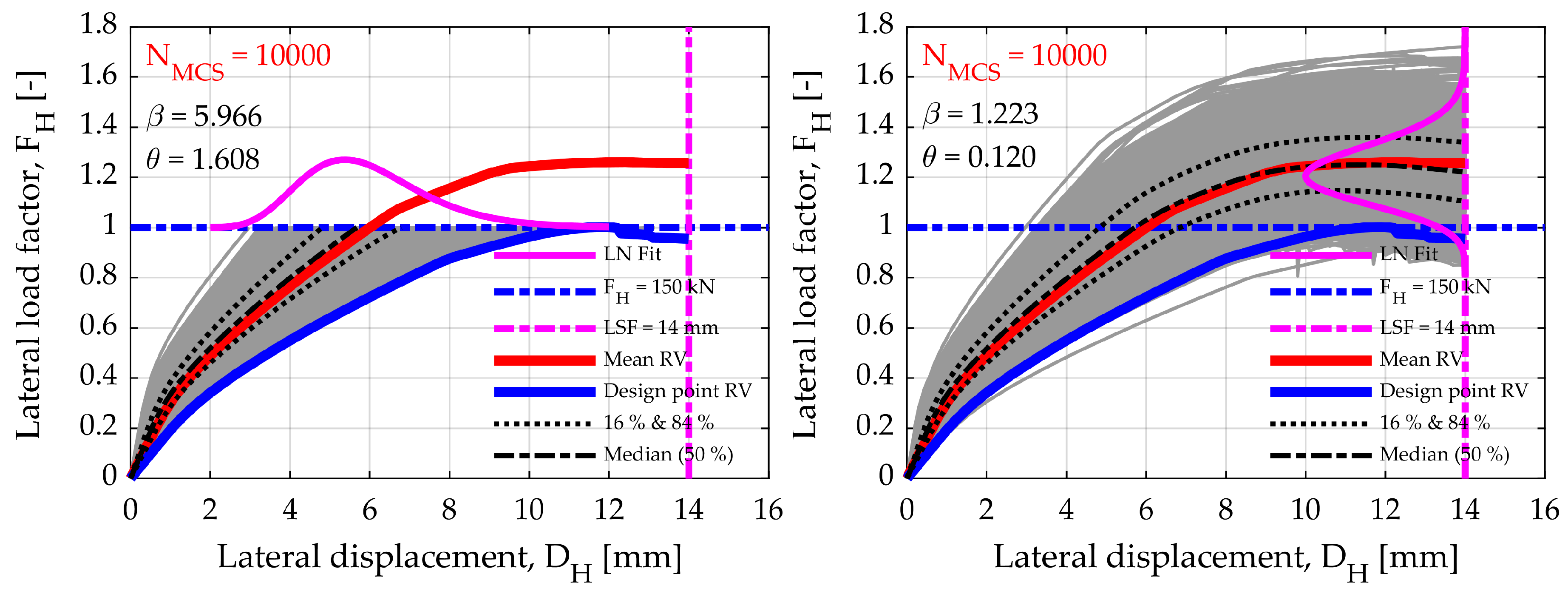
The results of the Monte Carlo analysis (conventional brute-force Monte Carlo) for the 10,000 simulation are presented below, carrying out a nonlinear analysis with Load Control (LC) of 150 kN in 40 steps per 5 kN (Figure 7). Figure 7 shows values of log-normal (LN) mean () and standard deviations (), and the diagrams are normalised based on horizontal force. The difference between the red and blue pushover curves should be noted. The red pushover curve was derived using the arithmetic mean values of all RV parameters. The blue pushover curve was based on the RV parameters obtained by FORM analysis ( values based on the Design Point) regarding the default LSF . As a by-product, FORM analysis provided importance measures ( and vectors in Table 2 and Table 3) to rank the uncertain parameters according to their relative influence on the structural reliability index, . Based on these importance vectors, FORM optimised the values of all RVs ( values), in which combination was exactly reached the Design Point or Most Probable Point (MPP). Thus, the difference between red and blue pushover curves is necessary and presents a useful product of the FORM analysis.
Given the complexity of the system, in Table 5 we can see that, for a sufficiently accurate calculation of the probability of exceeding the given LSF, 100,000 () simulations is recommended. Table 5 also shows the comparative values of the exceedance probability, , of the individual LSF, for the MCS and horizontal displacement of 14 mm, 10 mm and 6 mm, respectively, compared to the FORM analysis. It is evident that, with a relatively small number of MCS, it can be sufficiently accurate to predict the probability of exceeding the pre-defined limit state. In addition, values for the number of MCS lower than may vary significantly depending on the number of RV, complexity of the model and its degree of freedom.
Since simulations can be carried out in almost 5 min for this example (and the configuration of today’s average laptop), there is no reason to sacrifice the number of simulations and the accuracy of the reliability or sensitivity analysis itself. In this and more complex cases, a more rational Latin Hypercube Sampling (LHS) method would have to be considered, depending on the possibilities of the programming language, such as Python or MATLAB for compatibility reasons [45,46]. The effect of the MCS contribution to the number of simulations () in the significant nonlinear response domain of the numerical model is equally illustrated. For this purpose, pushover curves (load-displacement response) using MCS were computed with a displacement control (DC) incremental solution strategy (controlling displacement increment) to enable the model to converge in the negative stiffness domain (post-peak bearing capacity).
The displacement control was performed up to the 1.12% IDR, i.e., up to a 16 mm of horizontal displacement in 64 steps, making a step of 0.25 mm (Figure 7). The most important advantage of the displacement control is that we can track the contribution of the horizontal bearing capacity in a substantially nonlinear range, which in this case had a significant effect after a horizontal displacement greater than 6 mm, or IDR > 0.43%. It is interesting to see how some RVs parameters reflected the response of the model using an MCS, with displacement control up to 16 mm of horizontal displacement. It should be noted that the mean pushover curve, after a 1.0% IDR (14 mm), showed that the horizontal bearing capacity of the model stagnated (Figure 7). The following diagrams show the influence of individual parameter (while others were kept at their mean values) on the global nonlinear response of the numerical model. For example, in the first diagram, we can see that the effect of the yield strength of reinforcement steel () was only apparent after the global model yielding, which occurred at a horizontal load of kN, based on which these diagrams were normalised (showed by lateral load factor ). All diagrams for the impact of individual parameters are displayed for MCS. The red pushover curve is equal in all diagrams and shows the mean value of the pushover curve, with all parameters implemented with its arithmetic mean values.
Figure 8 shows 16th and 84th percentile values that were later used in the TDA. Figure 8 shows how much a particular parameter is sensitive to the contribution of the system’s horizontal bearing capacity, thus displaying vertical statistics at the 1.0% IDR level ( mm).
Figure 8 shows a dominance of significant parameters in a more pronounced nonlinear range: , , , , and , respectively. As a supplement to Figure 8, Figure 9 is added showing the sensitivity of individual RV in the form of standard deviation relative to the horizontal displacement, . It is interesting to see when certain parameters were activated with their contribution to the system’s bearing capacity. Notice the parameter at a horizontal displacement of 6 mm (0.43% IDR). Almost the same trend had the crushing concrete parameters , , , . It is interesting that almost none of the parameters related to the properties of concrete had a linear median curve due to significant softening effects. The following limits are also shown in Figure 9: the maximum reached a compressive strength limit of the unconfined concrete, and , the reinforcement yield strength limit, , and the limit as the beginning of concrete crushing, , and .
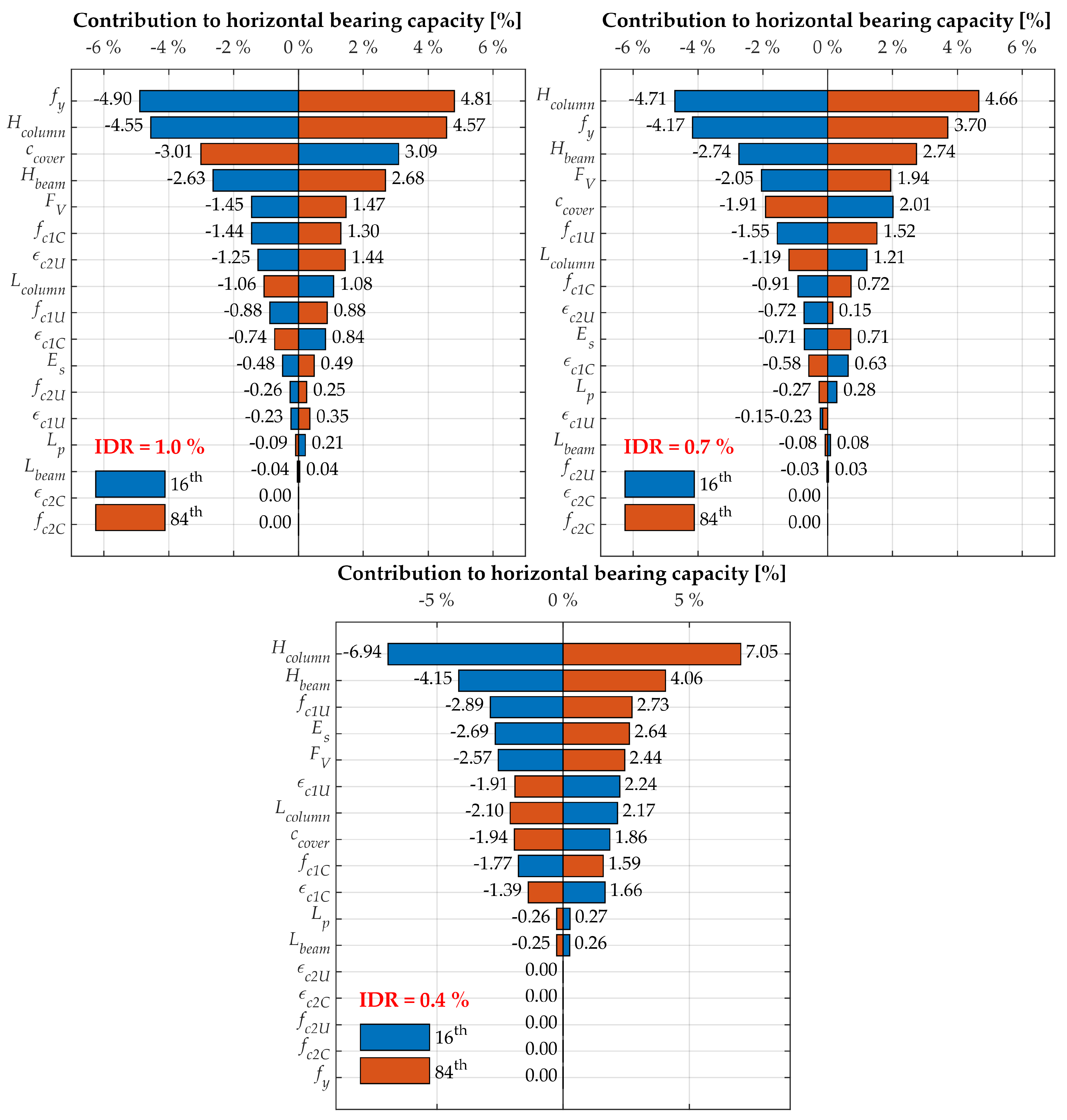
The tornado diagrams (Figure 10) were also constructed by applying the displacement control (DC) pushover analysis for deterministic sensitivity, which has become commonplace in reliability analysis of the field of earthquake engineering [31,32,41,42,43,47,48]. The TDA is a first-order sensitivity analysis. It comprises a set of horizontal bars, one for each input RV, whose lengths represent the variation of the EDP due to each considered input RV. The diagram is intuitive to read, and it helps the analyst identify which parameters to focus on. Each input variable is set to its median value (50th percentile), and the output is measured, establishing in this way a baseline output. One by one, each input parameter is fixed to both high and low extreme values of their probability distributions (generally corresponding to the 16th and 84th percentile, especially if the input distributions are different). The input parameters are ranked according to their absolute response difference (also called “swing”) so that the larger swing belongs to the variable producing the most significant uncertainty [43]. Repeated analyses observe the difference in the model response, in this case, the horizontal bearing capacity was represented in the percentage of response difference regarding the median pushover curve.
Since the overall response of the observed model is a combination of simulations of values with normal and log-normal distributions, the overall response was treated as log-normal distributions, thus we chose 16th and 84th percentile values. Figure 10 shows the different parameter importance for the three horizontal displacement limit states. Particularly noticeable the parameters that increase, compared to those that reduce the horizontal bearing capacity of the model (visible in Figure 10 in two different colours). In the predominant linear range of system behaviour (0.4% IDR), the effect of significant parameters responsible for influencing the initial stiffness of the system, such as , , , , , , and is visible. Parameters of crushed confined concrete did not contribute to any of the LSFs shown. For 0.4% IDR, the parameter did not affect the system’s bearing capacity, as expected, while for 1% IDR it was the main significant parameter affecting the system’s capacity. In the linear range, it is evident that the geometrical characteristics of the cross sections were the main contributors to the system’s bearing capacity ( and ) and the stiffness of constituent materials expressed as elastic modulus ( and defined as ).
6. Conclusions
This paper describes the reliability analyses of the RC frame by the FEM. The numerical model was based on and calibrated based on experimental testing of the single-bay single-storey planar RC frame at a scale of 1:2.5. The numerical model is shown in two variants, the nonlinear elements of which are defined by rotational springs (concentrated plasticity), and by the uniaxial fibre cross sections (distributed plasticity). Calibration of the numerical model was based on the cyclic hysteretic response of the frame, while the reliability analyses were based only the pushover bearing curve obtained by pushing the frame monotonously and unilaterally.
The ability to apply reliability analysis on a completely nonlinear numerical model using FEM and the comparability of MVFOSM, FORM, SORM-FP, and SORM-CF methods with MCS are what makes this study innovative. The MVFOSM analysis overestimated the reliability index by up to 52% compared to the FORM and SORM analyses that have proven to be comparable to the MCS. The FORM analysis gives insight into the importance of some parameters through the importance vectors without considering correlation () and considering correlation (). The SORM analysis with respect to the FORM analysis gave a smaller difference in the reliability index of the individual LSF, and that order was 0.13%, which is negligible. MCS gave accurate exceedance probabilities () of LSF for the number of simulations greater than , whereas this required number of simulations is expected to be significantly reduced by using sophisticated sampling techniques such as LHS. Significant parameters for the main LSF that is (horizontal statistics), based on the importance vectors , are: peak compression strength of the confined concrete (core), total depth of the column cross section, peak compression strength of the unconfined concrete (cover), beam length, tensile yield strength of reinforcing steel, and depth of the concrete cover directly affecting the effective cross-sectional depth. These six most important parameters are practically the same in importance if we do not observe the statistical correlation but are arranged in a different order. If we are interested in the contribution of the system’s bearing capacity, then we should emphasise that is the main governing parameter in vertical statistics, as demonstrated by the TDA.
As shown in Table 2, it is interesting that the beam length, , and thus the frame span, was the fourth most significant parameter, showing the importance of imperfections in the frame’s geometry, even with the low COV of 1%. In addition, parameters , and were the main and leading geometric parameters that control the frame response to the targeted design point. These results indicate the high influence of geometrical imperfections on the reliability of the RC structure. It was also noted that the depth of the concrete cover ranked high in importance, which is not surprising since its COV was 25% due to uncertainty in the construction of such structures. This finding may justify further investigation of the dispersion in the amount of cover in RC structures. The importance ranking of geometrical imperfections relative to other structural parameters indicated a significant influence of uncertain geometrical parameters on reliability assessments, even when the dispersion in the probability distribution is small.
These analyses can be used to minimise the total volume or the total expected cost of the structure subject to structural reliability constraints, to maximise the structural security subject to a given structural cost or simply to achieve a target structural reliability. This approach is particularly suitable for the possible implementation of geometric and material nonlinearities, the implementation of static and dynamic analysis, the simple coverage of aleatory (data-based) variability and epistemic (knowledge-based) uncertainty in terms of material and geometric characteristics, and earthquake time history records in the case of dynamic analysis. It is also possible to optimise significant Design Point-based parameters as well as to define multiple LSFs during the same analysis, which can be based on both local or global system responses, following internal forces and displacements or deformations. In the future, the authors suggest that individual RV should be individually assigned to each element separately, which is deliberately omitted in this study. In addition, as a guideline for future researchers, for similar construction systems, it is enough to conduct FORM analysis, where importance vectors are available, while, for greater flexibility and especially parametric studies in earthquake engineering, we prefer the use of MCS. MVFOSM proved to be very proximate and as such incorrect for the nonlinear model response, while the two SORM variants did not contribute to the accuracy of the reliability index.
Author Contributions
Conceptualisation, M.G. and A.G.; methodology, M.G. and A.G.; software, M.G. and J.I.; validation, M.G. and J.I.; formal analysis, M.G.; investigation, M.G.; resources, M.G. and A.G.; writing—original draft preparation, M.G., J.I. and A.G.; writing—review and editing, M.G., J.I. and A.G.; visualisation, M.G.; and supervision, M.G.
Funding
This paper was supported by Croatian Science Foundation (HrZZ) under the project UIP-2017-05-7113 Development of Reinforced Concrete Elements and Systems with Waste Tire Powder (ReCoTiP) [recotip.gfos.hr], and their support is gratefully acknowledged.
Acknowledgments
The research presented in this article is a part of the research project Development of Reinforced Concrete Elements and Systems with Waste Tire Powder—ReCoTiP [recotip.gfos.hr] supported by Croatian Science Foundation (HrZZ) and its support is gratefully acknowledged. The authors also acknowledge the constructive comments and suggestions provided by the anonymous reviewers, which improved the manuscript quality.
Conflicts of Interest
The authors declare no conflict of interest.
Abbreviations
The following abbreviations are used in this manuscript:
| COV | Coefficients Of Variation |
| CP | Concentrated Plasticity |
| DC | Displacement control |
| DCM | Ductility Class Medium |
| DOF | Degree-Of-Freedom |
| DP | Distributed Plasticity |
| E | Effect (Load) |
| EDP | Engineering Demand Parameter |
| FEM | Finite Element Method |
| FORM | First-Order Reliability Method |
| HLRF | Hasofer–Lind–Rackwitz–Fiessler |
| IDR | Inter-storey Drift Ratio |
| IM | Intensity Measure |
| LC | Load Control |
| LHS | Latin Hypercube Sampling |
| LN | Log-normal distribution |
| LSF | Limit State Function |
| MCS | Monte Carlo Simulation |
| MCS-DC | Monte Carlo Simulation, Displacement control |
| MCS-LC | Monte Carlo Simulation, Load control |
| MPP | Most Probable Point |
| MVFOSM | Mean-Value First-Order Second-Moment |
| N | Normal distribution |
| PACT | Performance Assessment Calculation Tool |
| PBEE | Performance-Based Earthquake Engineering |
| Probability Density Function | |
| PEER | Pacific Earthquake Engineering Research |
| PGA | Peak Ground Acceleration |
| R | Resistance (Bearing Capacity) |
| RC | Reinforced Concrete |
| RSM | Response Surface Method |
| RV | Random Variables |
| SDOF | Single Degree-Of-Freedom |
| SORM | Second Order Reliability Method |
| SORM-CF | Second-Order Reliability Method, Curvature Fitting |
| SORM-FP | Second-Order Reliability Method, First Principal Curvature |
| TDA | Tornado Diagram Analysis |
References
- Huang, C.; El Hami, A.; Radi, B. Overview of Structural Reliability Analysis Methods—Part I: Local Reliability Methods. Incert. Fiabil. Syst. Multiphys. 2017, 17, 1–10. [Google Scholar] [CrossRef]
- Hami, A.E.; Radi, B. Uncertainty and Optimization in Structural Mechanics; John Wiley & Sons, Inc.: Hoboken, NJ, USA, 2013; p. 138. [Google Scholar]
- Lemaire, M.; Chateauneuf, A.; Mitteau, J. Structural Reliability; ISTE Ltd., Wiley: Hoboken, NJ, USA, 2009; p. 485. [Google Scholar] [CrossRef]
- Grubišić, M. Models for Strengthening Assessment of Reinforced Concrete Frames by Adding the Infills for Earthquake Action. Ph.D. Thesis, University of Osijek, Faculty of Civil Engineering Osijek, Osijek, Croatia, 2016. [Google Scholar]
- McKenna, F.; Fenves, G.L.; Scott, M.H.; Mazzoni, S.; Jeremić, B. OpenSees—Open System for Earthquake Engineering Simulation; Technical report; Pacific Earthquake Engineering Research Centre, PEER, University of California: Berkeley, CA, USA, 2000. [Google Scholar]
- Datta, T.K. Seismic Analysis of Structures; John Wiley & Sons (Asia) Pte Ltd.: Singapore, 2010; p. 451. [Google Scholar] [CrossRef]
- Miranda, J. Structural Reliability Analysis with Implicit Limit State Functions; Technical Report; Instituto Superior Técnico, University of Lisbon: Lisbon, Portugal, 2013. [Google Scholar]
- Bozorgnia, Y.; Bertero, V. Earthquake Engineering: From Engineering Seismology to Performance—Based Engineering; CRC Press, ICC (International Code Council): Boca Raton, FL, USA, 2004. [Google Scholar]
- Deierlein, G.G.; Krawinkler, H.; Cornell, C.A. A Framework for Performance-Based Earthquake Engineering. Pac. Conf. Earthq. Eng. 2003, 273, 1–8. [Google Scholar] [CrossRef]
- Günay, S.; Mosalam, K.M. PEER Performance-Based Earthquake Engineering Methodology, Revisited. J. Earthq. Eng. 2013, 17, 829–858. [Google Scholar] [CrossRef]
- FEMA-P58/1. Seismic Performance Assessment of Buildings—Volume 1—Methodology; Technical Report; Applied Technology Council, Ed.; Federal Emergency Management Agency, FEMA & NEHRP: Washington, DC, USA, 2012.
- Sigmund, V.; Penava, D. Influence of Openings, with and Without Confinement, on Cyclic Response of Infilled R-C Frames—An Experimental Study. J. Earthq. Eng. 2014, 18, 113–146. [Google Scholar] [CrossRef]
- Kalman Šipoš, T.; Sigmund, V.; Hadzima-Nyarko, M. Earthquake performance of infilled frames using neural networks and experimental database. Eng. Struct. 2013, 51, 113–127. [Google Scholar] [CrossRef]
- Kabeyasawa, T.; Shiohara, H.; Otani, S.; Aoyama, H. Analysis of The Full–Scale Seven–Story Reinforced Concrete Test Structure. J. Fac. Eng. Univ. Tokyo Japan 1983, 37, 431–478. [Google Scholar]
- EN1992-1:2004. Eurocode 2—Design of Concrete Structures: General Rules and Rules for Buildings; European Committee for Standardization, CEN: Brussels, Belgium, 2004. [Google Scholar]
- EN1998-1:2004. Eurocode 8—Design of Structures for Earthquake Resistance—Part 1: General Rules, Seismic Actions and Rules for Buildings; European Committee for Standardization, CEN: Brussels, Belgium, 2004. [Google Scholar]
- Takeda, T.; Sozen, M.A.; Nielsen, N.N. Reinforced Concrete Response to Simulated Earthquakes. J. Struct. Div. 1970, 96, 2557–2573. [Google Scholar]
- Paulay, T.; Priestley, M.J.N. Seismic Design of Reinforced Concrete and Masonry Buildings, 1st ed.; Wiley, John Wiley & Sons, Inc.: Hoboken, NJ, USA, 1992; p. 735. [Google Scholar] [CrossRef]
- Scott, M.H.; Fenves, G.L.; McKenna, F.; Filippou, F.C. Software Patterns for Nonlinear Beam-Column Models. J. Struct. Eng. 2008, 134, 562–571. [Google Scholar] [CrossRef]
- Yaw, L.L. Co-Rotational Meshfree Formulation for Large Deformation Inelastic Analysis of Two-Dimensional Structural Systems. Ph.D. Thesis, University of California Davis, Davis, CA, USA, 2008. [Google Scholar]
- Denavit, M.D.; Hajjar, J.F. Description of Geometric Nonlinearity for Beam-Column Analysis in OpenSees; Technical report; Northeastern University: Boston, MA, USA, 2013. [Google Scholar]
- Rinchen; Hancock, G.J.; Rasmussen, K.J. Formulation and Implementation of General Thin-Walled Open-Section Beam-Column Elements in OpenSees; Technical Report 961; School of Civil Engineering, The University of Sydney: Sydney, Australia, 2016. [Google Scholar]
- Scott, M.H.; Fenves, G.L. Plastic Hinge Integration Methods for Force-Based Beam-Column Elements. J. Struct. Eng. 2006, 132, 244–252. [Google Scholar] [CrossRef]
- Scott, M.H.; Ryan, K.L. Moment-Rotation Behavior of Force-Based Plastic Hinge Elements. Earthq. Spectra 2013, 29, 597–607. [Google Scholar] [CrossRef]
- Haukaas, T.; Scott, M.H. Shape sensitivities in the reliability analysis of nonlinear frame structures. Comput. Struct. 2006, 84, 964–977. [Google Scholar] [CrossRef]
- Scott, M.H.; Haukaas, T. Software Framework for Parameter Updating and Finite-Element Response Sensitivity Analysis. J. Comput. Civ. Eng. 2008, 22, 281–291. [Google Scholar] [CrossRef]
- Scott, M.H. Evaluation of Force-Based Frame Element Response Sensitivity Formulations. J. Struct. Eng. 2011, 138, 72–80. [Google Scholar] [CrossRef]
- Deng, J.; Gu, D.; Li, X.; Yue, Z.Q. Structural reliability analysis for implicit performance functions using artificial neural network. Struct. Saf. 2005, 27, 25–48. [Google Scholar] [CrossRef]
- Hess, P.E.; Bruchman, D.; Assakkaf, I.A.; Ayyub, B.M. Uncertainties in Material and Geometric Strength and Load Variables. Nav. Eng. J. 2002, 114, 139–166. [Google Scholar] [CrossRef]
- Buonopane, S.G. Strength and Reliability of Steel Frames with Random Properties. J. Struct. Eng. 2008, 134, 337–344. [Google Scholar] [CrossRef]
- JCSS. Probabilistic Model Code Part III; Technical report; Technical University of Denmark, Joint Committee on Structural Safety (JCSS): Kongens Lyngby, Denmark, 2000. [Google Scholar]
- Celarec, D.; Ricci, P.; Dolšek, M. The sensitivity of seismic response parameters to the uncertain modelling variables of masonry-infilled reinforced concrete frames. Eng. Struct. 2012, 35, 165–177. [Google Scholar] [CrossRef]
- Ellingwood, B.; Galambos, T.; MacGregor, J.; Cornell, C.A. Development of a Probability—Based Load Criterion for American National Standard A58; Technical Report; National Bureau of Standards: Washington, DC, USA, 1980.
- El-Reedy, M.A. Reinforced Concrete Structural Reliability; CRC Press, Taylor & Francis Group: Boca Raston, FL, USA, 2013; p. 369. [Google Scholar]
- Robertson, L.E.; Naka, T. Tall Building Criteria and Loading; American Society of Civil Engineers: New York, NY, USA, 1980; p. 900. [Google Scholar]
- Mishra, D.K. Compressive Strength Variation of Concrete in a Large Inclined RC Beam by Non-Destructive Testing; Technical report; Associated Cement Companies Ltd.: Mumbai, India, 1990. [Google Scholar]
- Obla, K. Variation in Concrete Strength Due to Cement—Part III of Concrete Quality Series. Improv. Concr. Qual. 2014, 9, 7–16. [Google Scholar] [CrossRef]
- Sundararajan, C. Probabilistic Structural Mechanics Handbook: Theory and Industrial Applications; Springer: New York, NY, USA, 1995; p. 745. [Google Scholar] [CrossRef]
- Bartlett, F.M.; MacGregor, J.G. Assessment of Concrete Strength in Existing Structures; Technical Report; Department of Civil Engineering, University of Alberta: Edmonton, AB, Canada, 1994. [Google Scholar]
- Haukaas, T.; Kiureghian, A.D. Finite Element Reliability and Sensitivity Methods for Performance—Based Earthquake Engineering; Technical report, Pacific Earthquake PEER Report 2003/14; Engineering Research Centre, PEER, University of California: Berkeley, CA, USA, 2004. [Google Scholar]
- Porter, K.A.; Beck, J.L.; Shaikhutdinov, R.V. Sensitivity of Building Loss Estimates to Major Uncertain Variables. Earthq. Spectra 2002, 18, 719–743. [Google Scholar] [CrossRef] [Green Version]
- Celarec, D.; Dolšek, M. The impact of modelling uncertainties on the seismic performance assessment of reinforced concrete frame buildings. Eng. Struct. 2013, 52, 340–354. [Google Scholar] [CrossRef]
- Porter, K. A Beginner’s Guide to Fragility, Vulnerability, and Risk; Technical report; University of Colorado Boulder: Boulder, CO, USA; SPA Risk LLC: Denver, CO, USA, 2019. [Google Scholar]
- EN1990-1:2002. Eurocode 0—Basis of Structural Design; European Committee for Standardization, CEN: Brussels, Belgium, 2002. [Google Scholar]
- Python. Python Language Reference; Version 3.6.8, [MSC v.1916 64 bit (AMD64)]; Python Software Foundation: Wilmington, DE, USA, 2018. [Google Scholar]
- MATLAB. The MathWorks, Inc.; Version 9.4 (R2018a); The MathWorks, Inc.: Natick, MA, USA, 2018. [Google Scholar]
- Lee, T.H.; Mosalam, K.M. Probabilistic Seismic Evaluation of Reinforced Concrete Structural Components and Systems; Technical report, PEER Report 2006/04; Pacific Earthquake Engineering Research Centre, College of Engineering, PEER, University of California: Berkeley, CA, USA, 2006. [Google Scholar]
- Huang, Y.; Whittaker, A.S.; Luco, N. Performance Assessment of Conventional and Base-Isolated Nuclear Power Plants for Earthquake and Blast Loadings; Technical Report MCEER-08-0019; University of Buffalo: Buffalo, NY, USA, 2008. [Google Scholar]
Figure 1.
Schematic representation of geometry, cross sections and the amount of reinforcement (left) and crack development during the cyclic test (right).
Figure 1.
Schematic representation of geometry, cross sections and the amount of reinforcement (left) and crack development during the cyclic test (right).

Figure 2.
The hysteresis curve (left) and the average of two backbone curves as well as the secant stiffness curve, K (right).
Figure 2.
The hysteresis curve (left) and the average of two backbone curves as well as the secant stiffness curve, K (right).
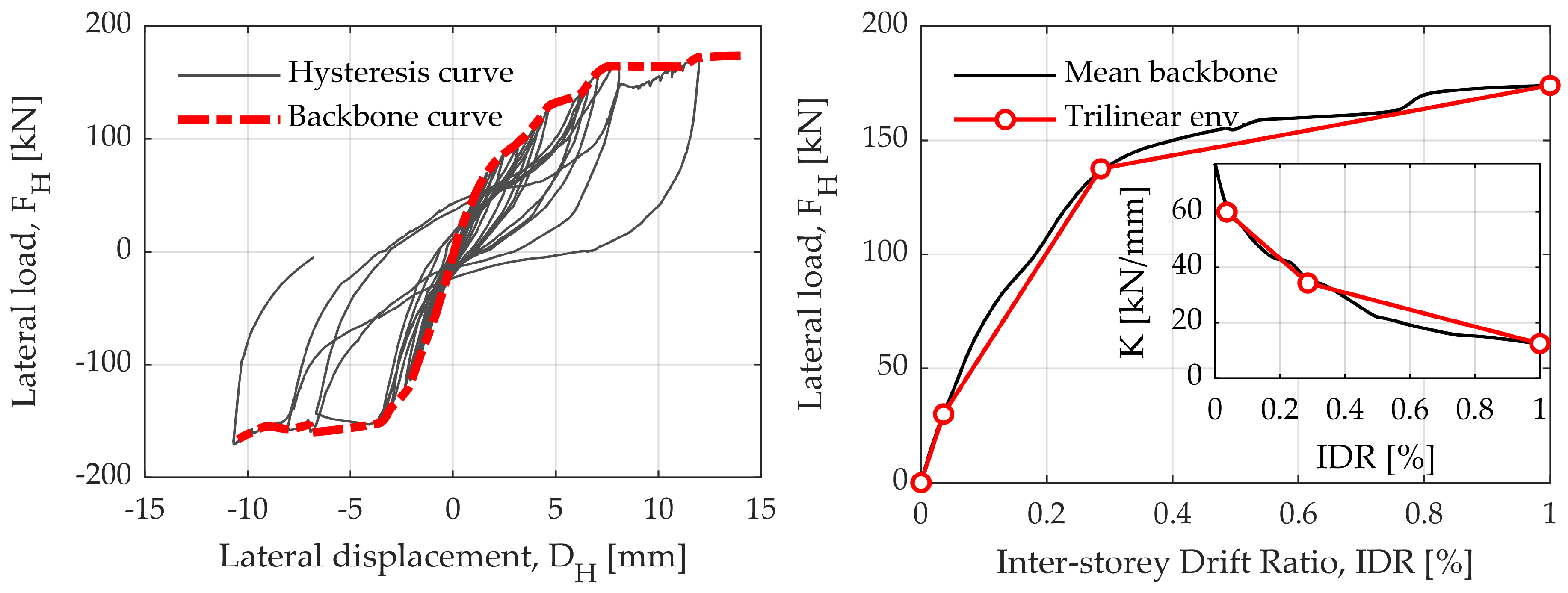
Figure 3.
Experimental displacement history, indicating the extremes of individual cycles and numerical displacement control.
Figure 3.
Experimental displacement history, indicating the extremes of individual cycles and numerical displacement control.
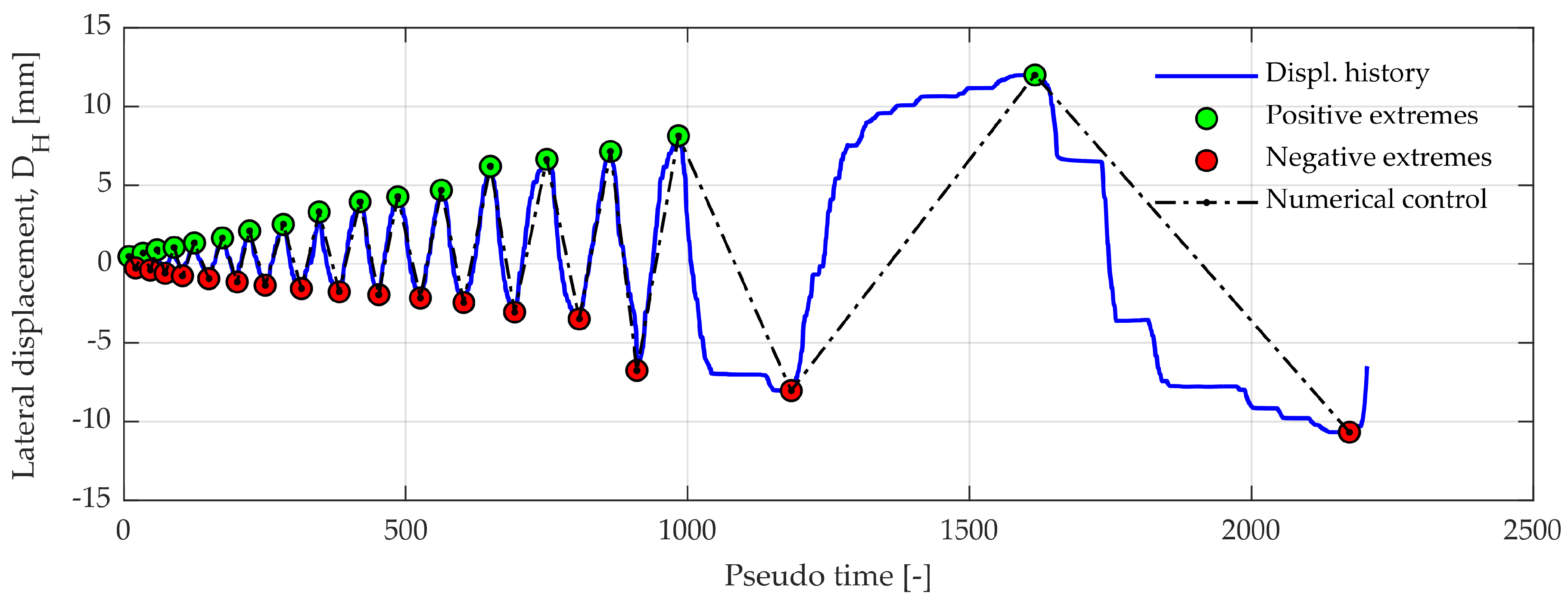
Figure 4.
Numerical model configuration scheme: calibration of hysteresis behaviour—concentrated plasticity with Takeda hysteresis rules (above) and for reliability analysis—distributed plasticity (under).
Figure 4.
Numerical model configuration scheme: calibration of hysteresis behaviour—concentrated plasticity with Takeda hysteresis rules (above) and for reliability analysis—distributed plasticity (under).

Figure 5.
Comparison of the numerical hysteresis curve with the experimental hysteresis response (left) and numerical pushover curve with the experimental mean backbone curve (right), both for the concentrated (lumped) plasticity model.
Figure 5.
Comparison of the numerical hysteresis curve with the experimental hysteresis response (left) and numerical pushover curve with the experimental mean backbone curve (right), both for the concentrated (lumped) plasticity model.
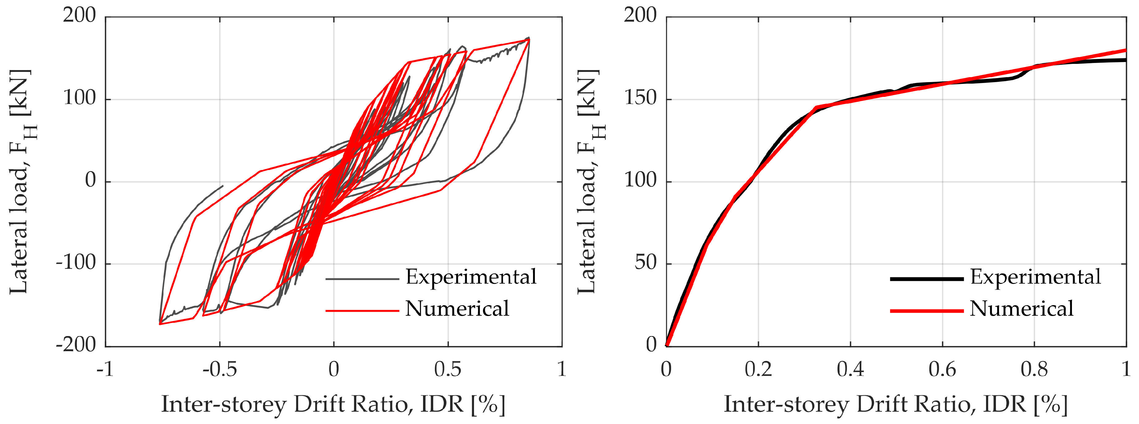
Figure 6.
Comparison of hysteresis curve with pushover curve for distributed plasticity model (DP), with corresponding drift limit and horizontal load level at reinforcement yielding.
Figure 6.
Comparison of hysteresis curve with pushover curve for distributed plasticity model (DP), with corresponding drift limit and horizontal load level at reinforcement yielding.
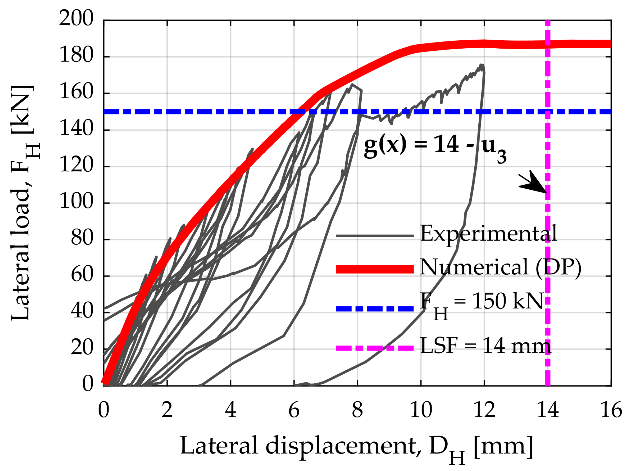
Figure 7.
Illustration of MCS, for simulations, load control MCS-LC (left) and displacement control MCS-DC (right).
Figure 7.
Illustration of MCS, for simulations, load control MCS-LC (left) and displacement control MCS-DC (right).

Figure 8.
Overview of the influence of individual RV on the nonlinear response of the RC frame (MCS-DC), at the level of the pushover curve.
Figure 8.
Overview of the influence of individual RV on the nonlinear response of the RC frame (MCS-DC), at the level of the pushover curve.
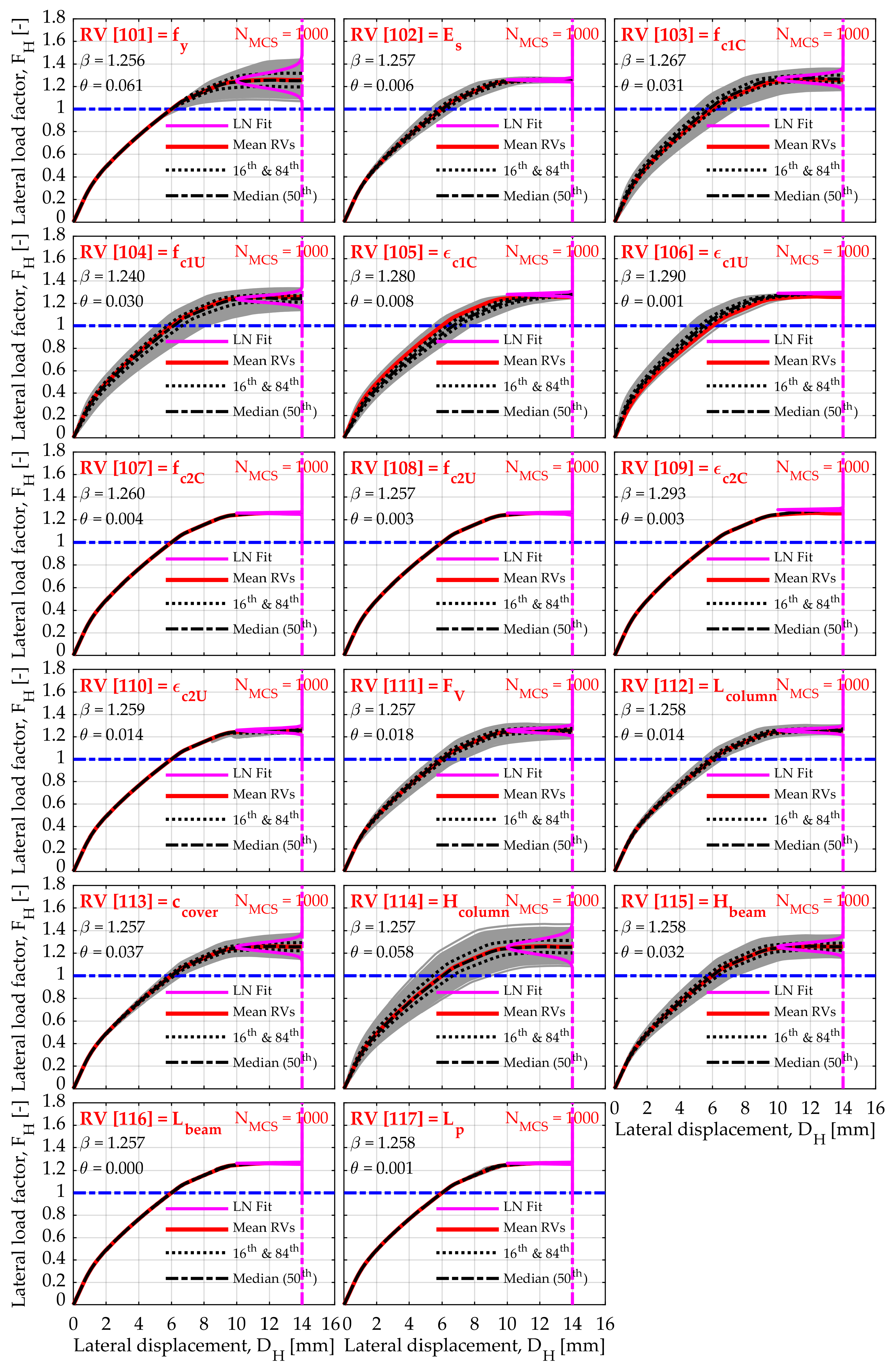
Figure 9.
Overview of the sensitivity of individual RV on the nonlinear response of the RC frame (MCS-DC), in the form of standard deviations () with respect to the horizontal displacement ().
Figure 9.
Overview of the sensitivity of individual RV on the nonlinear response of the RC frame (MCS-DC), in the form of standard deviations () with respect to the horizontal displacement ().
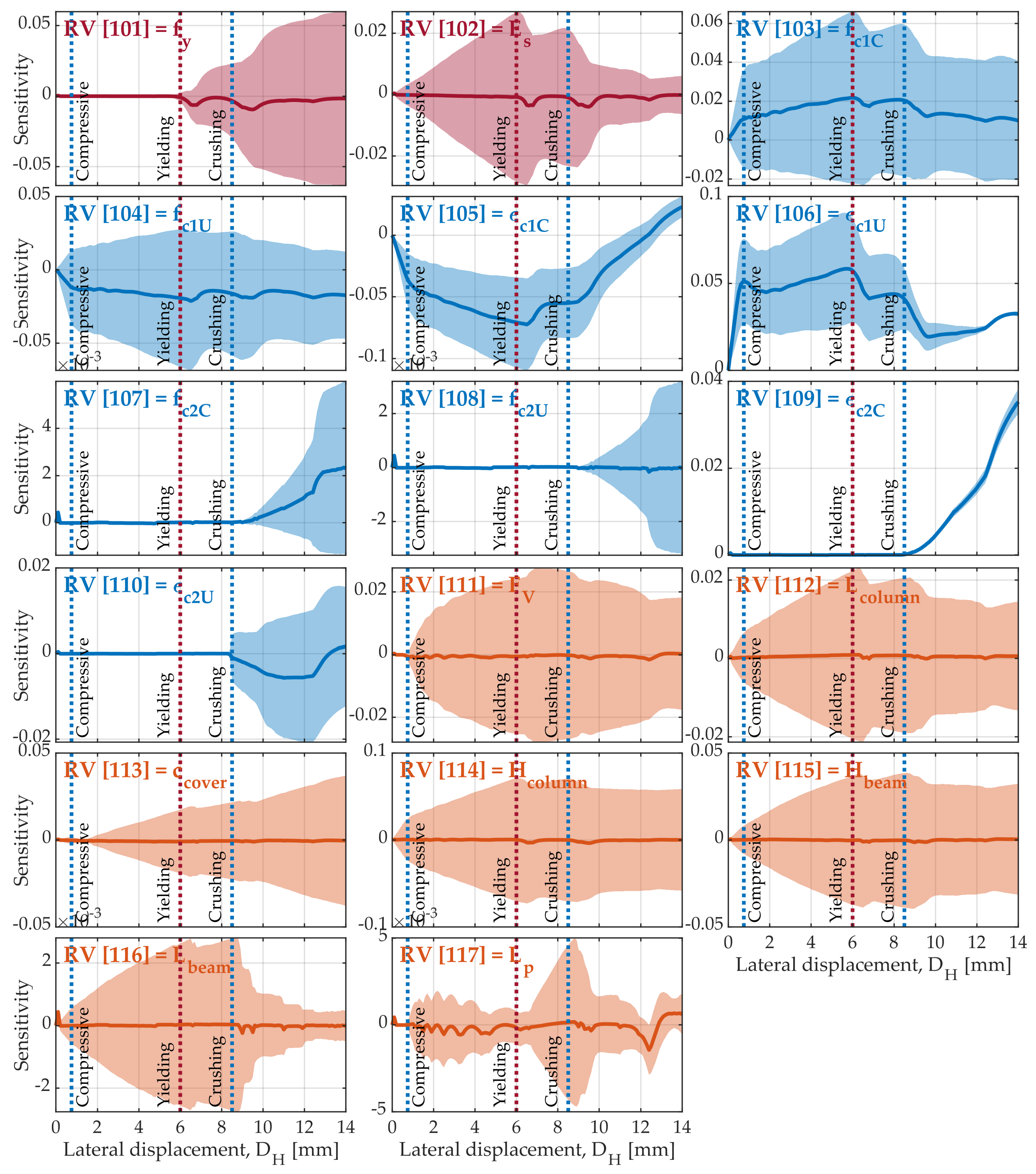
Figure 10.
Tornado diagrams for three LSFs, showing the contribution of individual variables to horizontal bearing capacity.
Figure 10.
Tornado diagrams for three LSFs, showing the contribution of individual variables to horizontal bearing capacity.

Table 1.
Summary of RVs with its mean values (), standard deviations () and coefficients of variation (COV).
Table 1.
Summary of RVs with its mean values (), standard deviations () and coefficients of variation (COV).
| RV | Param. | Mean, | St. Dev., | COV | Units | Distr. | References for COV |
|---|---|---|---|---|---|---|---|
| 101 | 550 | 44 | 0.08 | (MPa) | LN | Experiment + [30,31,32] | |
| 102 | 210,000 | 12,600 | 0.06 | (MPa) | LN | Experiment + [26,29,30] | |
| 103 | −65 | −9.75 | 0.15 | (MPa) | N | Experiment + [30,33,34,35,36] | |
| 104 | −0.005 | −0.0008 | 0.15 | (−) | N | Experiment + [30,33,34,35,36,37] | |
| 105 | −50 | −7.5 | 0.15 | (MPa) | N | Experiment + [30,33,35,36] | |
| 106 | −0.002 | −0.0003 | 0.15 | (−) | N | Experiment + [30,33,37] | |
| 107 | −11.5 | −2.3 | 0.20 | (MPa) | N | Experiment + [30,33,34,35,36] | |
| 108 | −0.0085 | −0.0017 | 0.20 | (−) | N | Experiment + [30,33,34,35,36,37] | |
| 109 | −10 | −2 | 0.20 | (MPa) | N | Experiment + [30,33,35,36] | |
| 110 | −0.0035 | −0.0007 | 0.20 | (−) | N | Experiment + [30,33,37] | |
| 111 | 365 | 36.5 | 0.10 | (kN) | N | Experiment + [32,34] | |
| 112 | 1400 | − | 0.01 | (mm) | N | [30,34,38] | |
| 113 | 15 | − | 0.25 | (mm) | N | [30,34,38] | |
| 114 | 200 | − | 0.05 | (mm) | N | [30,34,38] | |
| 115 | 200 | − | 0.05 | (mm) | N | [30,34,38] | |
| 116 | 2000 | − | 0.01 | (mm) | N | [30,34,38] | |
| 117 | 15 | − | 0.10 | (mm) | N | [30,34,38] |
Table 2.
The rank of RVs and parameters by importance vectors, obtained from the FORM analysis, according to the vector, i.e., considering the correlation between the defined RVs for the LSF .
Table 2.
The rank of RVs and parameters by importance vectors, obtained from the FORM analysis, according to the vector, i.e., considering the correlation between the defined RVs for the LSF .
| Param. | Units | Mean, | Design Point, | Importance, | Importance, | |
|---|---|---|---|---|---|---|
| RV 103 | (MPa) | |||||
| RV 114 | (mm) | |||||
| RV 104 | (MPa) | |||||
| RV 116 | (mm) | |||||
| RV 101 | (MPa) | |||||
| RV 113 | (mm) | |||||
| RV 115 | (mm) | |||||
| RV 109 | (−) | |||||
| RV 111 | (kN) | |||||
| RV 112 | (mm) | |||||
| RV 110 | (−) | |||||
| RV 102 | (MPa) | |||||
| RV 107 | (MPa) | |||||
| RV 108 | (MPa) | |||||
| RV 105 | (−) | |||||
| RV 117 | (mm) | |||||
| RV 106 | (−) |
Table 3.
The rank of RVs and parameters by importance vectors, obtained from the FORM analysis, according to the vector, i.e., not considering the correlation between the defined RVs for the LSF .
Table 3.
The rank of RVs and parameters by importance vectors, obtained from the FORM analysis, according to the vector, i.e., not considering the correlation between the defined RVs for the LSF .
| Param. | Units | Mean, | Design Point, | Importance, | Importance, | |
|---|---|---|---|---|---|---|
| RV 103 | (MPa) | |||||
| RV 114 | (mm) | |||||
| RV 101 | (MPa) | |||||
| RV 116 | (mm) | |||||
| RV 109 | (−) | |||||
| RV 113 | (mm) | |||||
| RV 115 | (mm) | |||||
| RV 111 | (kN) | |||||
| RV 112 | (mm) | |||||
| RV 102 | (MPa) | |||||
| RV 104 | (MPa) | |||||
| RV 107 | (MPa) | |||||
| RV 105 | (−) | |||||
| RV 110 | (−) | |||||
| RV 117 | (mm) | |||||
| RV 108 | (MPa) | |||||
| RV 106 | (−) |
Table 4.
Comparison of the reliability indexes (and its probabilities) for MVFOSM, FORM, SORM-FP and SORM-CF analysis for three different LSF.
Table 4.
Comparison of the reliability indexes (and its probabilities) for MVFOSM, FORM, SORM-FP and SORM-CF analysis for three different LSF.
| Analysis | Reliability Index, | LSF #1, mm | LSF #2, mm | LSF #3, mm |
|---|---|---|---|---|
| MVFOSM | () | 4.816 | 2.511 | 0.205 |
| FORM | () | 3.161 | 2.304 | 0.318 |
| SORM–FP | () | 3.161 | 2.304 | 0.318 |
| SORM–CF | () | 3.165 | 2.310 | 0.321 |
Table 5.
Comparison of the number of Monte Carlo Simulation (MCS-LC), together with the FORM analysis, on the exceedance probability of an LSF.
Table 5.
Comparison of the number of Monte Carlo Simulation (MCS-LC), together with the FORM analysis, on the exceedance probability of an LSF.
| Total MCS, | LSF #1, mm, | LSF #2, mm, | LSF #3, mm, | Running Time (h:m:s) |
|---|---|---|---|---|
| 50 | 0.0000 | 0.0000 | 0.2560 | 0:00:01 |
| 100 | 0.0000 | 0.0000 | 0.2720 | 0:00:02 |
| 250 | 0.0000 | 0.0032 | 0.3424 | 0:00:03 |
| 500 | 0.0016 | 0.0040 | 0.2896 | 0:00:04 |
| 1000 | 0.0008 | 0.0048 | 0.3288 | 0:00:06 |
| 2500 | 0.0016 | 0.0048 | 0.3072 | 0:00:11 |
| 5000 | 0.0013 | 0.0059 | 0.3102 | 0:00:22 |
| 10,000 | 0.0006 | 0.0064 | 0.3077 | 0:00:39 |
| 100,000 | 0.0008 | 0.0068 | 0.3058 | 0:06:23 |
| 500,000 | 0.0008 | 0.0072 | 0.3024 | 0:35:20 |
| 0.0000 | 0.0060 | 0.4186 | 0:00:01 | |
| 0.0008 | 0.0106 | 0.3751 | 0:00:03 | |
| 0.0008 | 0.0106 | 0.3751 | 0:00:06 | |
| 0.0008 | 0.0105 | 0.3741 | 0:00:19 |
© 2019 by the authors. Licensee MDPI, Basel, Switzerland. This article is an open access article distributed under the terms and conditions of the Creative Commons Attribution (CC BY) license (http://creativecommons.org/licenses/by/4.0/).
Share and Cite
MDPI and ACS Style
Grubišić, M.; Ivošević, J.; Grubišić, A. Reliability Analysis of Reinforced Concrete Frame by Finite Element Method with Implicit Limit State Functions. Buildings 2019, 9, 119. https://0-doi-org.brum.beds.ac.uk/10.3390/buildings9050119
AMA Style
Grubišić M, Ivošević J, Grubišić A. Reliability Analysis of Reinforced Concrete Frame by Finite Element Method with Implicit Limit State Functions. Buildings. 2019; 9(5):119. https://0-doi-org.brum.beds.ac.uk/10.3390/buildings9050119
Chicago/Turabian StyleGrubišić, Marin, Jelena Ivošević, and Ante Grubišić. 2019. "Reliability Analysis of Reinforced Concrete Frame by Finite Element Method with Implicit Limit State Functions" Buildings 9, no. 5: 119. https://0-doi-org.brum.beds.ac.uk/10.3390/buildings9050119
Note that from the first issue of 2016, this journal uses article numbers instead of page numbers. See further details here.