A Sliding Mode Control Strategy for an ElectroHydrostatic Actuator with Damping Variable Sliding Surface


1
Laboratory of Aerospace Servo Actuation and Transmission, Beihang University, Beijing 100191, China
2
School of Mechanical Engineering and Automation, Beihang University, Beijing 100191, China
3
School of Transportation Science and Engineering, Beihang University, Beijing 100191, China
4
School of Mechanical and Electrical Engineering, Lanzhou University of Technology, Lanzhou 730050, China
*
Author to whom correspondence should be addressed.
Actuators 2021, 10(1), 3; https://0-doi-org.brum.beds.ac.uk/10.3390/act10010003
Submission received: 16 November 2020
/
Revised: 19 December 2020
/
Accepted: 22 December 2020
/
Published: 25 December 2020
(This article belongs to the Section Actuators for Manufacturing Systems)
Abstract
:Electro-hydrostatic actuator (EHA) has significance in a variety of industrial tasks. For the purpose of elevating the working performance, we put forward a sliding mode control strategy for EHA operation with a damping variable sliding surface. To start with, a novel sliding mode controller and an extended state observer (ESO) are established to perform the proposed control strategy. Furthermore, based on the modeling of the EHA, simulations are carried out to analyze the working properties of the controller. More importantly, experiments are conducted for performance evaluation based on the simulation results. In comparison to the widely used control strategies, the experimental results establish strong evidence of both overshoot suppression and system rapidity.
1. Introduction
Electro-hydrostatic actuator (EHA) is considered a good solution in a wide range of industrial applications such as spacecraft [1], aircraft [2], robotics [3,4,5,6], vehicles [7], and heavy-duty suspension [8]. As a highly integrated power transmission system, EHA outperforms traditional hydraulic systems by decreasing the weight and increasing the working efficiency [9]. Typically, an electro-hydrostatic actuator (EHA) is a self-contained, pump-controlled system that is composed of a motor, a pump, a supercharged fuel tank, and a hydraulic cylinder (for simplification, the “hydraulic cylinder” is referred to as a “cylinder” in the rest of the paper) [10]. As such, by removing the hydraulic lines and servo valves, the system weight associated with the hydraulic tubing and the fluid is eliminated [11], while the system maintainability and reliability is improved [12]. As reported in [13], “The last level of individualization is the separate assignment of the EHA systems to each actuator. This configuration combines the best features of both hydraulic and electric technologies.”
Advances are ongoing to improve the working performance of hydraulic servo actuators. In the actuating domain, the nonlinearity and time variation of EHA have an impact on the dynamics as well as the servo control accuracy [14]. Research is still in progress to mitigate the deficiencies. Control strategy is one such field, with recent publications highlighting the significance of adaptive control (AC) [15], fuzzy control (FC) [16], feedback linearization control (FLC) [17], sliding mode control (SMC), and its improved extension, e.g., merging with proportion integration differentiation (PID) control [18,19], cascade control (CC) [20], etc.
In an effort to address dynamic properties, current controlling applications mainly focus on exploring the potential of resolving the system uncertainties [21]. Encouragingly, the sliding mode controller, due to its simple, robust, and accurate method of action, has attracted a great deal of interest as one of the best controllers. The integration of related algorithms, such the New Adaptive Reaching Law (NARL) [19] against chattering and the extended state observer (ESO) [22] for working condition estimation, is verified. State observers are commonly applied to control systems for the tasks of system uncertainties estimation and compensation [23,24,25]. In addition, Gao et al. constructed a two-stage sliding mode control to retain its rapidity and employed an improved Lyapunov function to reduce system chattering [26]. Ren and Zhou presented a sliding mode controller with a fuzzy logic reasoning strategy, which provides faster adjustment time and higher accuracy [27]. Notwithstanding, the problem of system overshoot caused by the large inertia arises in heavy-duty operating applications where the stable actuating of EHA under load has important performance implications. Specifically, the contradiction between system rapidity and overshooting, as the main concern, is most pronounced when establishing a control strategy [28]. Previous works used to take a smooth curve as an alternative of the step signal in SMC [19,22]. In other words, an intact step input will cause the signal jump in SMC, in which case a slow-settling output is formed to get a smaller overshoot [21].
For establishing an optimal control strategy for EHA operation, we propose a novel sliding mode control with damping variable sliding surface (DV-SMC) strategy. On the one hand, this control strategy aims at tackling the contradiction between settling time and the overshoot with high robustness. On the other hand, the tuning of sliding mode surface parameters for DV-SMC is put forward. Together with the controller, an extended state observer is also designed to estimate and compensate for the control strategy. In line with EHA controlling, our controller, as a competitive alternative, can give rise to even better working performance. The contributions of this paper are as follows:
- (1)
- To alleviate the conflict between the overshoot and rapidity of the EHA system, a control strategy based on SMC is proposed. Compared to the classical SMC method, the overshoot is suppressed without undermining the speed, which is in line with both simulative and experimental results.
- (2)
- For parameter adjustment, a parameter-tuning method for SMC is established. For the controller, damping-ratio-based parameter tuning is optimized, which further improves the industrial applications of our controller.
Following the introduction, this research introduces background knowledge on EHA in Section 2, describes the proposed DV-SMC strategy in Section 3, shows the modeling and simulating outcomes in Section 4, provides experimental results and analysis in Section 5, and finally presents conclusions and future research directions in Section 6.
2. Prerequisite
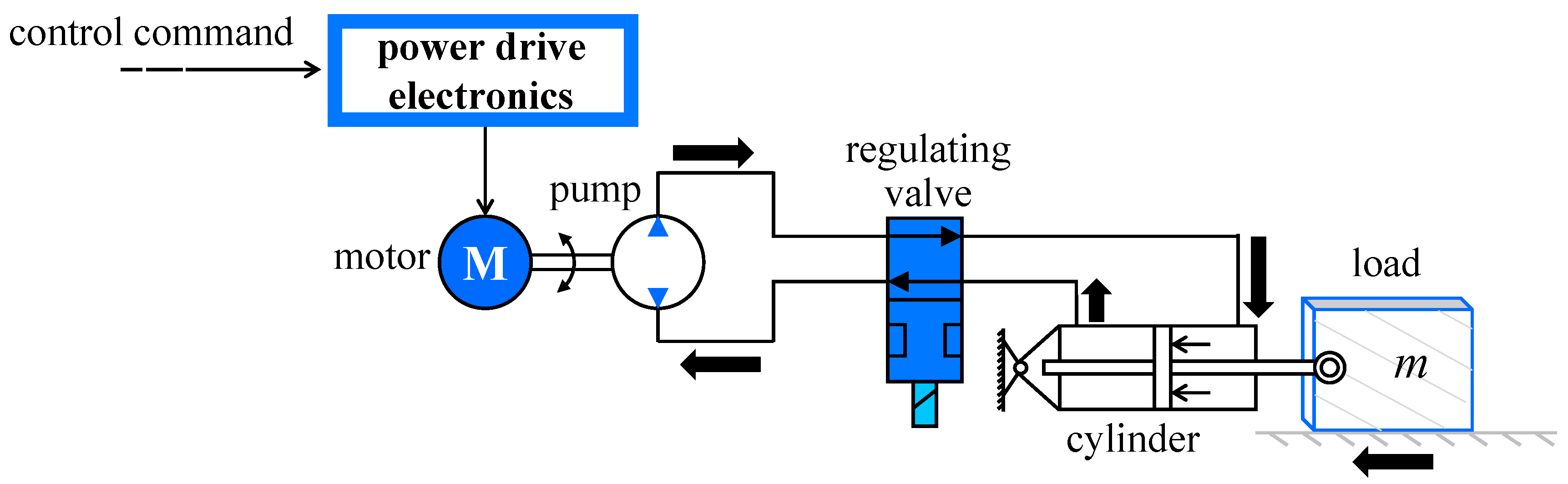
Figure 1 presents the working principle of the EHA. As mentioned above, the main components of an EHA are a motor, a bidirectional pump, and an oil cylinder connected by meter-in and meter-out valves. Specifically, a motor-driven pump without power transmission being hindered is employed; therefore, inefficient servo valves are eliminated [29]. As a rule, the EHA performs flow rate control by a pump coupled to a motor. In Figure 1, the bold arrows indicate the flow of hydraulic oil. The control command, which drives the motor to rotate forward, is sent via the power drive electronics. Thus, oil is pumped into the right chamber of the cylinder, which generates pressure and makes the cylinder move to the left. Likewise, the reverse rotation of the motor leads to the left-to-right movement of the cylinder. That is, the load is driven by the moving of the cylinder for manipulating an individual actuator. Accordingly, a closed control loop can be formed.
The modeling of the motor and the cylinder is presented as follows.
2.1. Brushless DC Motor (BLDCM) Model
We employ a brushless DC motor (BLDCM), which is of high reliability, to drive the pump in this research. Supposing the BLDCM is of Y-connection, the winding can be mathematically described as follows:
where U,L, and R represent the equivalent voltage, inductance, current, and resistance; Ke is the back-electromotive force (EMF) coefficient; Te is the corresponding electromagnetic torque of the motor; Jm is the moment of inertia of the motor; Tl is the equivalent external load; and Bm is the viscous friction coefficient.
2.2. Pump-Controlled Cylinder Model
Let Qi and Qo be the inlet and outlet flow of plunger pump. The working flow of the EHA can be modeled as follows:
where Dp is the pump displacement; Li and Lo represent the internal and external leakage coefficients; pi, po, and pa are the inlet pressure, outlet pressure, and back pressure of the oil tank pump; Vin and Vout are the equivalent inlet and outlet volume; and βe is the elastic modulus of the fluid.
Similarly, the dynamic model of the pump-controlled cylinder is denoted as follows:
where the subscripts l and r indicate the left- and right-hand sides of the cylinder chambers, respectively; A is the effective area of the piston rod; x is its displacement; and Lc stands for the internal leakage.
Due to the short flow passage inside the valve, the pressure loss within it is negligible. Notably, based on the flow continuity theorem, we have:
Thus, the model of the cylinder, by combining Equations (4) and (5), is defined as follows:
In Equation (5), Vo represents the effective volume of the chamber; La is proportional to the pressure difference Δp is the total leakage coefficient of the pump and the cylinder; Qa is the unconsidered flow loss; M stands for the total equivalent mass of the cylinder and the load; Bc is the viscous friction coefficient of the cylinder; Ks is the elastic load coefficient; Ff stands for the static friction; and FL is the load.
Based on Equations (1) and (5), is established to characterize the system state, from which the EHA model can be written as follows:
where Ja stands for the total rotational inertia of the motor and the pump.
2.3. Problem Formulation
According to Equation (6), x4 is a virtual control input with respect to the EHA model, based on which a three-order subsystem is formed by the first three equations. It can be observed that this high-order system contains both matched disturbances and mismatched disturbances. SMC is used to guarantee the robustness but is insensitive to mismatched disturbances [30,31]. Specifically, the control with mismatched disturbances is more challenging than that with only matched disturbances, and only a few related results have been proposed [32].
In this way, we now redefine the state variables as . Apparently, z1 z2 and z3 represent the position, velocity, and acceleration of the cylinder, respectively. Hence, the first three terms from Equation (6) can be elaborated on by Equation (7):
where
and
such that Qun stands for the flow loss that has not been considered.
3. Methodology
The proposed DV-SMC consists of two parts, i.e., a novel sliding mode controller design and an extended state observer design. A stability analysis is presented as well.
3.1. Sliding Mode Controller with Damping Variable Sliding Surface
Originally, SMC was an approach for nonlinear controlling [33,34]. As pointed out in Section 1, the basic SMC shows great robustness against parameter uncertainties despite its failure to deal with perturbations. Seeing as methods for attenuating the perturbations are both productive and effective, we employed the exponential approach law to remove the perturbations and invoke the robustness of SMC [35,36].
On this occasion, a molded sliding mode controller is developed first. The system errors together with the derivatives are:
Then, we choose the sliding surface σ as follows:
where c1 and c2 are positive, which meets the requirements of the Routh‒Hurwitz stability criterion [37]. The error e, as such, approaches 0 during the control process.
Moreover, the exponential approach law is applied, which leads to:
Furthermore, with u* representing the target value of the virtual control variable, we have
In Equations (12)–(14), the variation of c1 and c2 with respect to the controlling is restricted to c1, c2 > 0. Despite the range of c1 and c2 within a two-dimensional plane, the values of these two parameters will inevitably affect the dynamic performance.
At this stage, we set the right side of Equation (12) to 0 to construct a transfer function between x and xd, which is:
where s is the laplacian operator.
A typical evaluation is to trace a step signal. In this case, as long as Xd is nonderivable at the start time, and do not exist in theory. However, in reality, and will converge to the largest number instead of diverging to infinity. Furthermore, the enormous number can cause a saturation of control output (u* in Equation (14)) and a plunge of output following the step moment, which results in an impact. However, this impact is the source of a large overshoot or an oscillation during the system adjustment process. For this reason, the overshoot is limited by an artificial ceiling of and , as mentioned in Section 1.
Therefore, assuming that both and are 0 in the step response, the corresponding transfer function is:
Notably, the transfer function in Equation (16) denotes a standard second-order oscillation. Consequently, computation with c1 and c2 is facilitated by introducing the undamped natural frequency ωn and the damping ratio ξ, which are:
One of the key facts is that the smaller ξ is, the faster the system response and the larger the overshoot and oscillation that will be generated. Otherwise, the increase in ξ can restrain the oscillation at the cost of settling time. Considering the contradiction between rapidity and stability, the damping ratio of 0.707 is a solution to a certain extent. In contrast, if the damping ratio is a changeable parameter, i.e., a small ξ for establishing system rapidity during the initial sliding and a large one for suppressing the overshoot in the end, an even better response is possible.
Thus, we optimize the sliding surface presented in Equation (12):
where and represent the minimum and maximum damping ratio and is the sensitivity factor for damping ratio regulating.
Thereafter, we can rewrite the transfer function from Equation (16) as follows:
We have the system error e, starting with the sliding, as , and . In this way, the damping ratio for the initial control phase is , which indicates an underdamped state with fast response. With the controlling system approaching its equilibrium, we have , while the damping ratio increases and finally reaches .
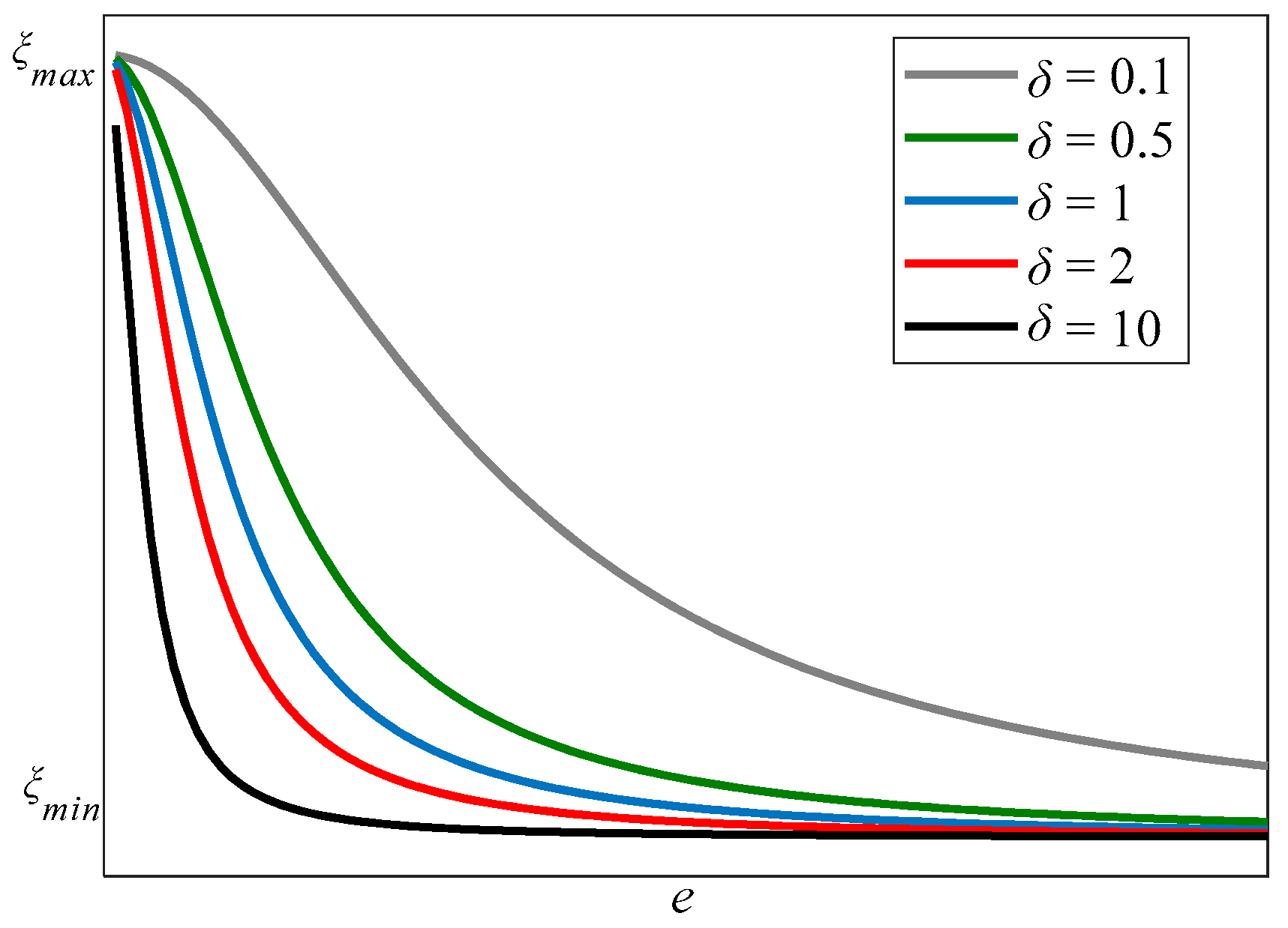
Accordingly, the adaptive regulation of ξ, within the interval , can cater to the needs of system rapidity and stability via an optimal damping ratio. The sensitivity factor is employed to determine the speed of the working damping ratio approaching its upper and lower limits. When increases, ξ moves toward , and otherwise to (see Figure 2).
Then, in relation to the system parameter variation, we can compute the control output based on the virtual control variable. From Equation (14), we can compute the control law as follows:
3.2. Extended State Observer (ESO)
State estimation requires knowledge of the plant, the control input, and the sensing signals [38]. As presented in Equation (7), the EHA model is equivalent to a pure integral series system. Specifically, the parameter z1 is measured by a displacement sensor, from which z2 and z3 are derived by using a differentiator. The noise generated by the differentiator will cause the distortion of z2 and z3. Moreover, let stand for the system disturbance, which is compensated for by the robust term in Equation (13). Nevertheless, this compensation is such an overcompensation that it can bring cause chattering in the steady phase of the servo system. For this reason, a fourth-order ESO, not only for estimating the system state, but also for revising the compensation via observing the system disturbance, is established in Equation (22):
where , while is the gain matrix of ESO and is Hurwitz.
The total disturbance observed by ESO is:
The estimation error formula of ESO can be obtained with Equations (22) and (7), and is
where stands for the estimation error and is bounded by .
3.3. Stability Analysis
This is an example of an equation: The stability analysis starts with taking the derivation of Equation (19):
Replacing the true values with the observed values, we have:
Basically, to investigate the system stability, a Lyapunov candidate [39] is considered:
together with
Substituting Equation (21) into Equation (25) gives:
and we define it as follows:
With such a definition, we can also rewrite Equation (34) as follows:
It is clear that and are polynomials with state variables and , where and .
Hence, from Equation (28), we have
Conforming to the convergence presented in Equation (30), the proposed observer has the following characteristics: the state variable can converge toward its true value . Sequentially, and will finally approach 0, which is also the condition for . As a result, when there is a sufficiently large , the result of can be obtained. Recall that in Equation (32) is not designed to fully compensate for the external disturbance . Notably, the here is far smaller than the in Equation (14). Similarly, the robust item in Equation (21) is far smaller than that in Equation (14). As expected, the sliding mode chattering can thereby be reduced.
The proof of control stability is complete. The DV-SM controller, together with the ESO, can respond to the demand of existence and reachability in line with the Lyapunov theory, which indicates that the proposed control strategy can be applied to the EHA operation.
4. Numerical Simulations
4.1. Model Establishing
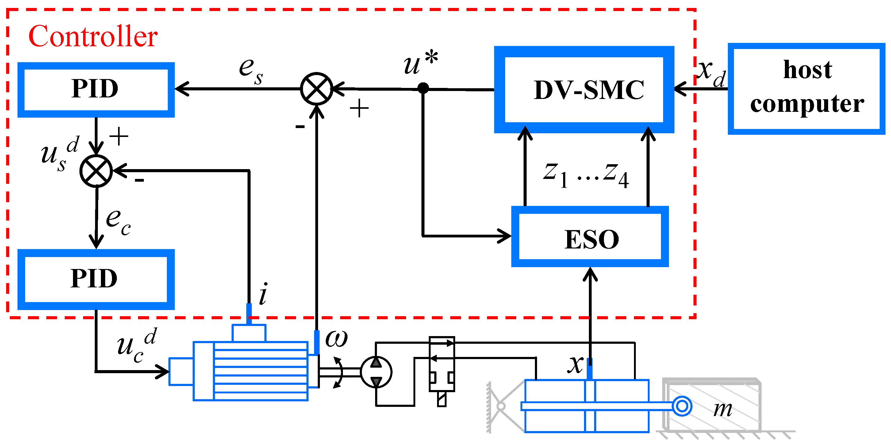
Numerical simulations are carried out to find suitable settings for the proposed DV-SMC strategy. In this research, a double-loop PID control scheme is taken as a representative example, which is implemented on the EHA together with the controller and its ESO. Specifically, a cascade control strategy is developed whereby the outer loop contains a DV-SM controller and the inner loop consists of a double-loop PID controller. The block diagram of the cascade controller is presented. As shown in Figure 3, the acquisition of sensors is in real time, e.g., position x and current i. After the controller receives xd from the host computer, DV-SMC collects the state variables, i.e., zi (i = 1,2,3,4), from ESO to generate the output u*. Consequently, the final output, which is exactly represented by ucd, is calculated by dual-PID.
Bounded by the model of EHA in Equation (6), a second-order system with the input of voltage and output of motor spindle speed is constructed, as is the case for the double-loop PID controller. We have:
where the subscripts s and c indicate the speed loop and the current loop, respectively; stands for the control output of the current loop; and is the error of that loop. For PID control, , , and are the proportional coefficient, integral coefficient, and differential coefficient, respectively.
The configuration of the proposed EHA for simulation is given in Table 1.
4.2. Model Simulation Results
In order to verify the superiority of the DV-SMC strategy, an EHA system is built and operated on MATLAB/Simulink software published by MathWorks. Inc. (Natick, MA, USA) with the same simulating input, different control strategies are conducted.
The control effect of three different strategies, i.e., three-loop PID control (labeled as “PID”), SMC with double-loop PID control (labeled “SMC”), and the proposed DV-SMC with double-loop PID control (labeled “DV-SMC”), is compared to the reference input. Specifically, the inner loop of all three controllers is the same, which is double-loop PID. For the simulation, step signals of 50 mm, 15 mm, and 5 mm are sent to the system as a reference for assessing the system tracking performance. As shown in Figure 4, the black solid line represents the reference control input, while the blue dotted line, red dotted line, and solid green line stand for the PID control, SMC, and DV-SMC, respectively.
In Figure 4, the conventional PID control fails to keep up with the various step signals. Through integration with the SMC and the DV-SMC, the tracking performance effect of the controller can be improved. The main reason for that is the system compensation as well as the robustness against disturbance. On evaluating the settling time and the overshoot, we compare SMC and DV-SMC in line with the same input. Clearly, comparable results are obtained in terms of the settling time for both controllers. In contrast, the DV-SM controller is a better alternative for overshoot suppression. Giving an optimal damping ratio of 0.707, the maximum overshoot of the SM controller is 12%, 6.7%, and 6.7% for the three reference inputs, respectively. On the other hand, there is no overshoot generated within DV-SMC under each condition. Notably, the optimal damping ratio corresponds to SMC and still results in an over 5% overshoot during the sliding phase. A possible explanation is that the impact when approaching the sliding surface in the initial stage will cause an overshoot in controlling. Since the proposed controller employs the adaptive regulation of damping ratio, it is reasonable to expect a better overshoot suppression effect. The overdamping, based on the adaptive regulation of the damping ratio, can significantly restrain the overshoot when the error approaches 0 during the sliding process.
4.3. Damping Ratio Selection
As pointed out in Section 3.1, the real damping ratio of the controller ranges from to . Corresponding simulations are carried out to figure out the values between and .
Let be the starting state to convey the deviation of e toward 0. Recall that the damping ratio close to 0 indicates a better working performance in the initial phase according to Equation (20). Thus, we have:
Equation (33) means that the actual damping ratio is determined not only by the sensitivity factor but also by the maximum value of the deviation e. We set as a constant and . Suppose we have at the sliding surface, with smaller than the effective stroke of EHA. During the sliding process, the value of increases rapidly, conforming to the drop in e.
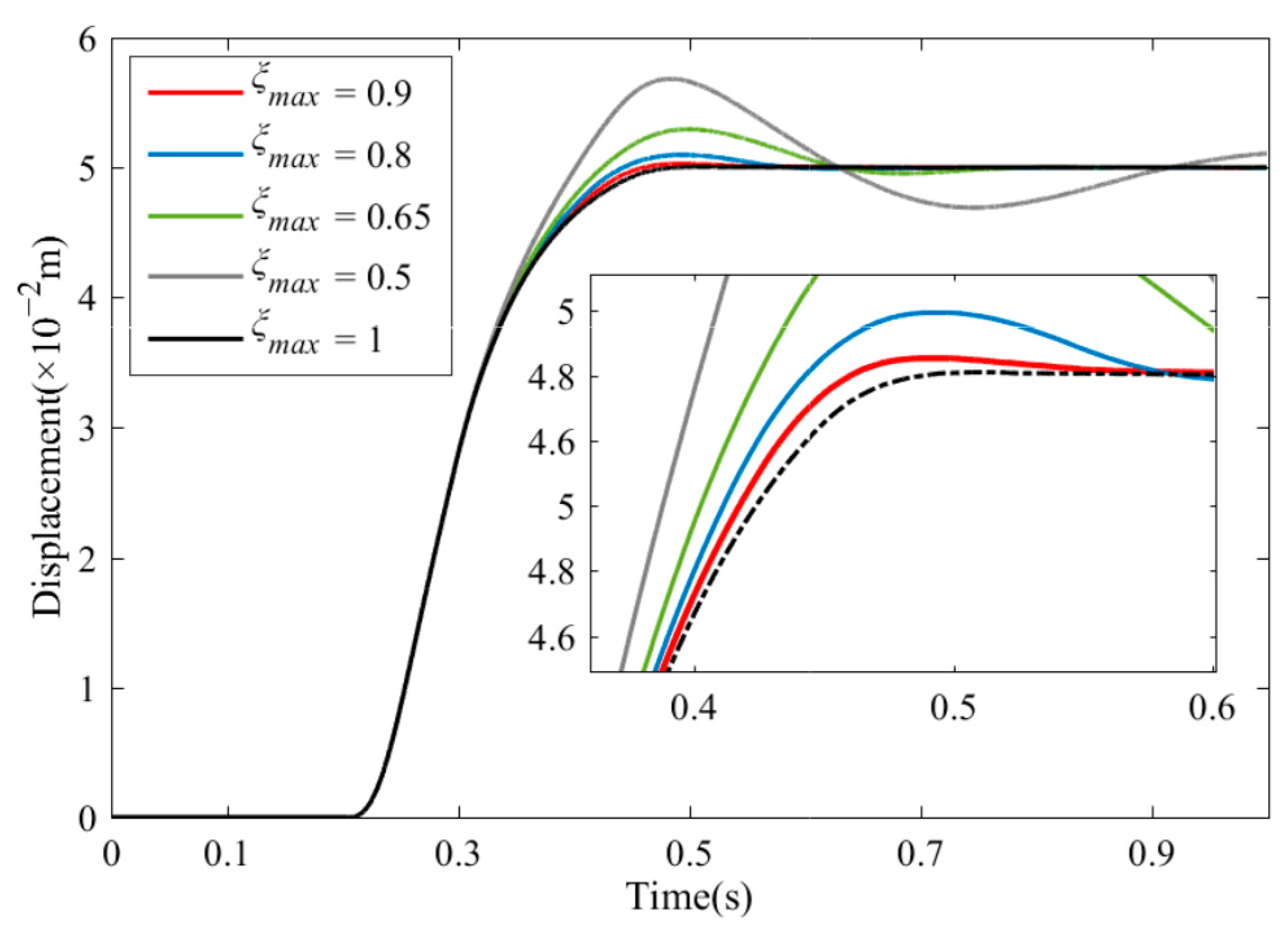
Likewise, identifies its significance in the response of the second half. The value of works on the effects of the system state approaching equilibrium point and the final suppression on overshoot. We set the values of to 0.5, 0.65, 0.8, 0.9, and 1. The step response of different is illustrated in Figure 5. The simulating outcomes show that the increasing damping ratio results in a decrease in the second-half overshoot and the adjustment time. We see that the settling time drops from 0.8 s to 0.3 s, with increasing from 0.5 to 1. Simultaneously, the overshoot is suppressed by about 20%. Based on performance comparison, the configuration of within the interval [0.8,1] can be applied for practical use. The of 0.8 can meet the demands of a steady response with a small amount of overshoot. For a system expecting a quick response without any overshoot, the value of is set to 1.
5. Experiments
5.1. Experimental Settings
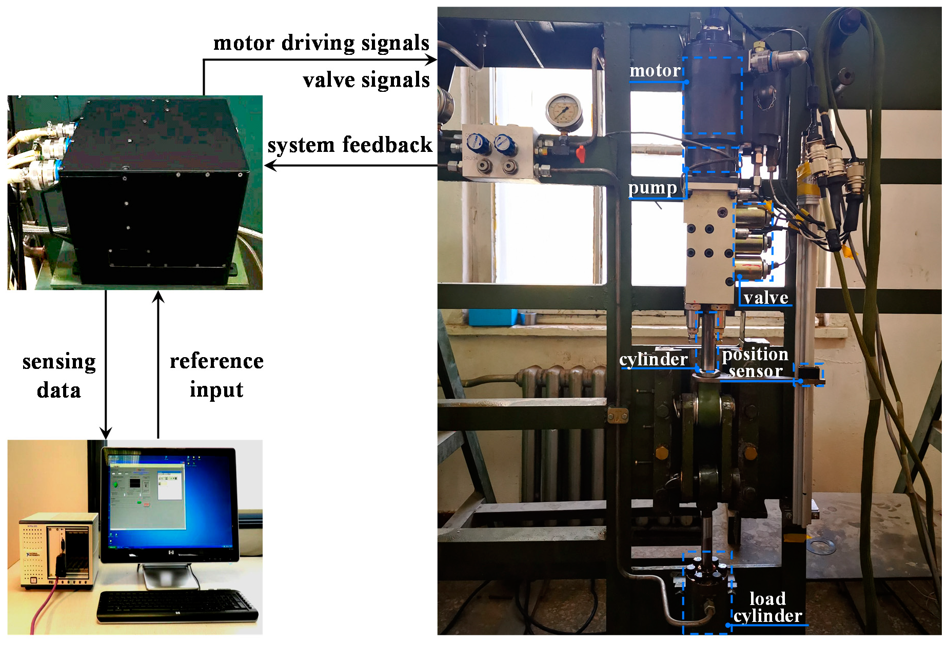
Aiming to verify the working performance of the proposed control strategy, we conduct the experiments with dedicatedly manufactured prototypes. Figure 6 shows the test rig. In this work, a prototype of the EHA is built for testing. The displacement of the actuator is detected by a position sensing element, while the sensing signals are transmitted to the controller via an encoder of SG37-2-09.52. Moreover, two pressure sensors are employed for monitoring the pressure of the two piston cylinder chambers. The regulating valves are carried out for working mode switching, together with other experimental apparatus for facilitate the testing (Figure 6). More details of the EHA are given in Table 2.
Control commands, with 200 Hz sampling frequency, are originally performed on a host computer as the reference input conforming to the computational simulation. Power electronics are established for signal exchanging and processing. The control command is delivered from the host computer to the power electronics and then to the EHA as the system inputs. Specifically, the inputs of EHA consist of motor driving signals and valve signals. The former is generated by integrating the control commands and the system feedback, while the latter switches the operation mode. The system feedback, containing the motor current and the cylinder displacement, is sent back to the host computer via the power electronics. In this experiment, the feedback data are derived from a second-order Butterworth filter with a 40 Hz cutoff frequency, which is five times the referenced bandwidth of the EHA.
5.2. Results
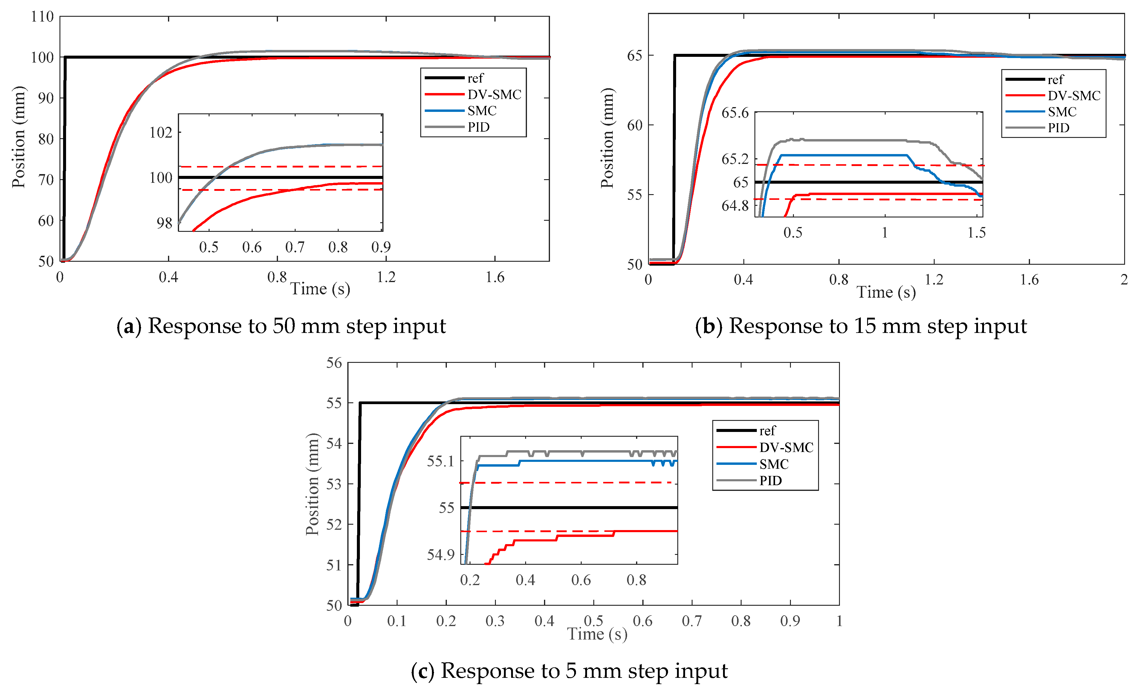
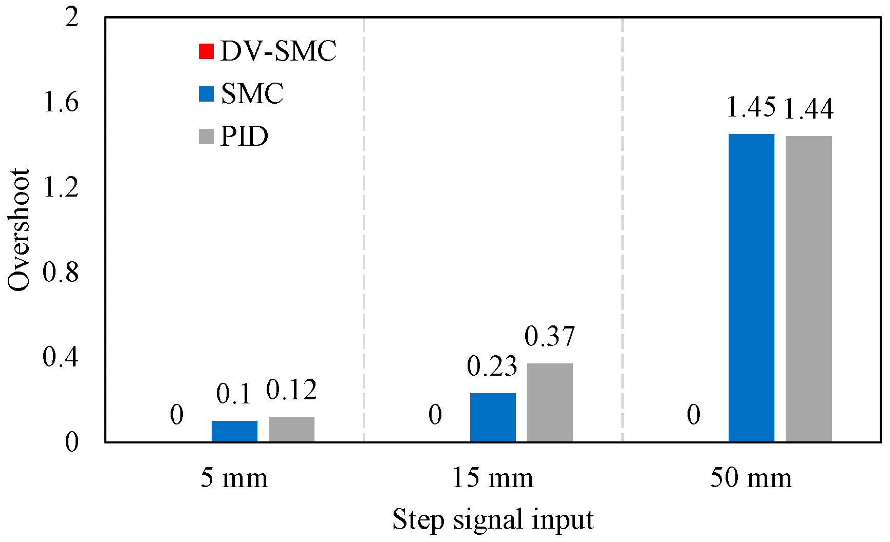
A 5000 N external load is applied to the cylinder of the EHA beforehand. Based on the simulating results, we refer to the control inputs as 5 mm, 15 mm, and 50 mm step signals and apply the reference inputs to the three controllers, i.e., the PID controller, the SM controller, and the DV-SM controller mentioned in Section 4.2. Figure 7 shows the results of the controlling tasks carried out using all reference inputs. In these figures, all the controllers obtain a trend consistent with the simulation outcomes. To further validate the working properties, the overshoot and settling time of different controllers are presented in Figure 8 and Figure 9.
The PID controller and SM controller achieved almost the same responses in both tests. In contrast, the proposed DV-SM controller outperformed other control strategies in all evaluation settings. There was no overshoot generated by the DV-SM controller. The minimum performance gap of 1.53% can be observed in Figure 8 against the SMC with a 15 mm step signal input (0.23 mm vs. 15 mm). In line with the simulation, is set to 1, while is 0. By regulating the damping ratio within this range, the system output oscillation is significantly weakened. Furthermore, the ESO also facilitates the controlling process. Thus, our controller is capable of eliminating overshoot. For this reason, the DV-SMC strategy is the best approach in terms of suppressing the system overshoot.
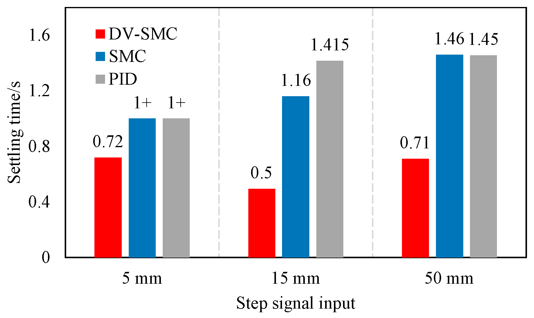
Consistent results are obtained for the settling time comparison. For system rapidity description, we define a settling time as the first time to stabilize within the range of reference input. In Figure 9, one can see that the proposed DV-SMC is still the best-performing resolution among the three controllers. The explanation for this issue is quite similar to that of the simulation results. The overshoot occurs because of saturated output of SMC and PID as well as the inertia of the workload. In contrast, the DV-SMC strategy maintains its output when it first reaches the controlling accuracy range. As shown in Figure 9, in terms of settling time, the proposed DV-SMC still exceeds the performance of the other methods.
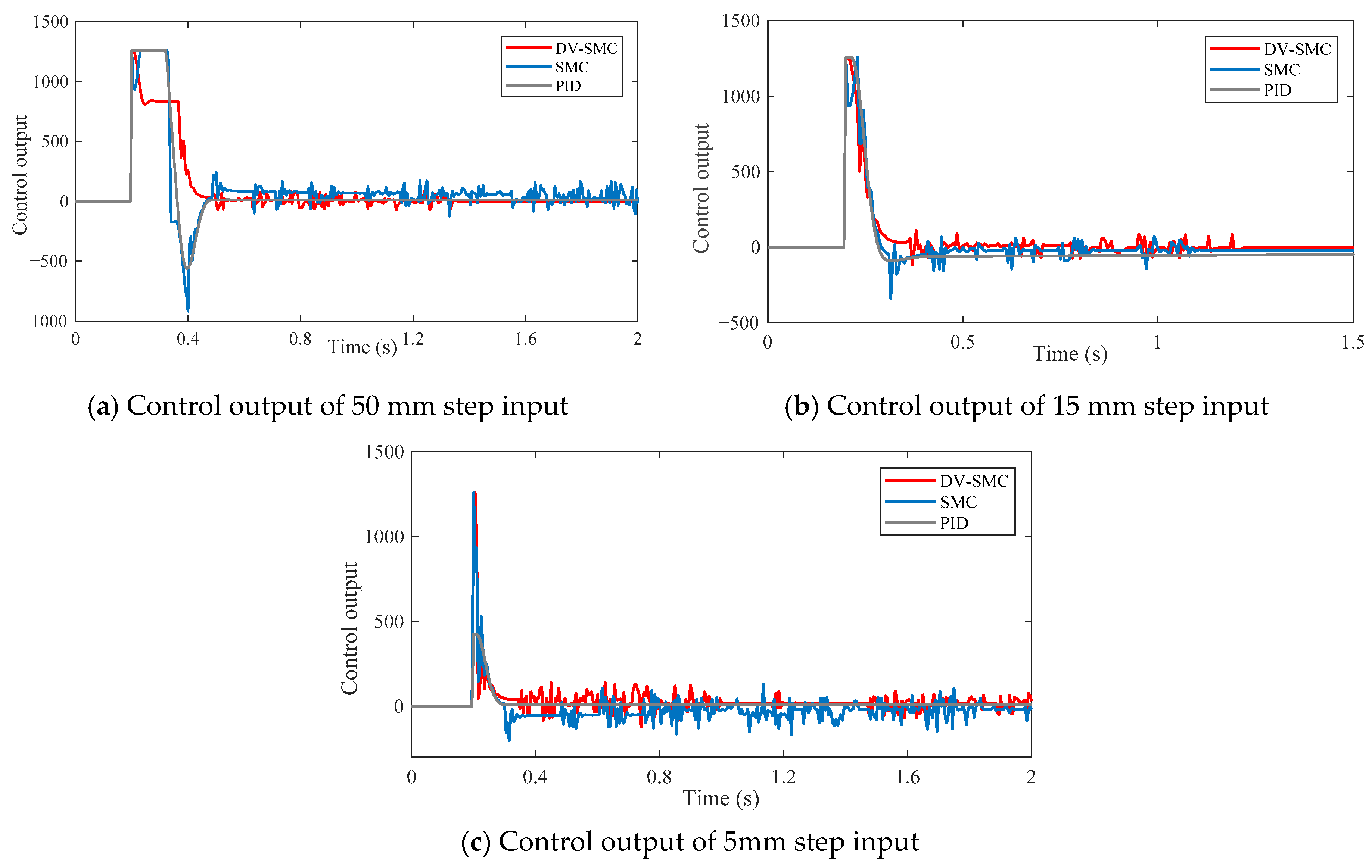
Regarding the controlling outputs, results show the stability of the three controllers; see Figure 10. Generally, DV-SMC withdraws the output saturation and reaches the stabilization within a short time. Corresponding to the system response, our method is superior in overshoot suppression and reverse output preclusion. During the steady-state phase, the sign function pre-proposed in (26) is replaced by a saturation function in Equation (34). It is worth noticing that the system oscillation is significantly restrained, with the control output fluctuating slightly.
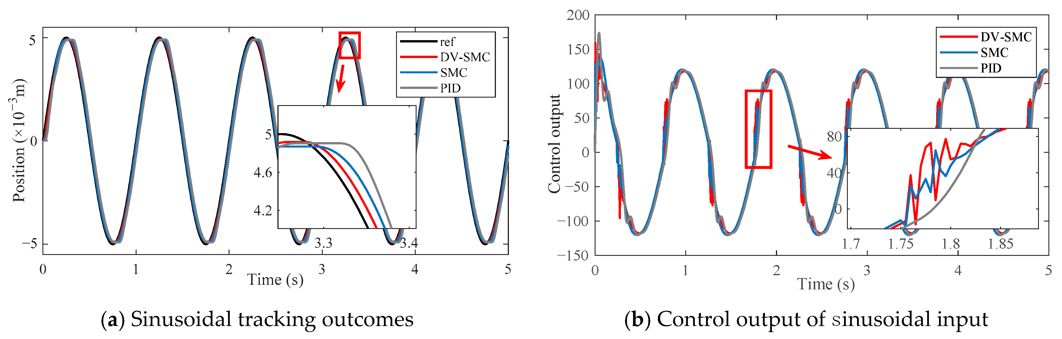
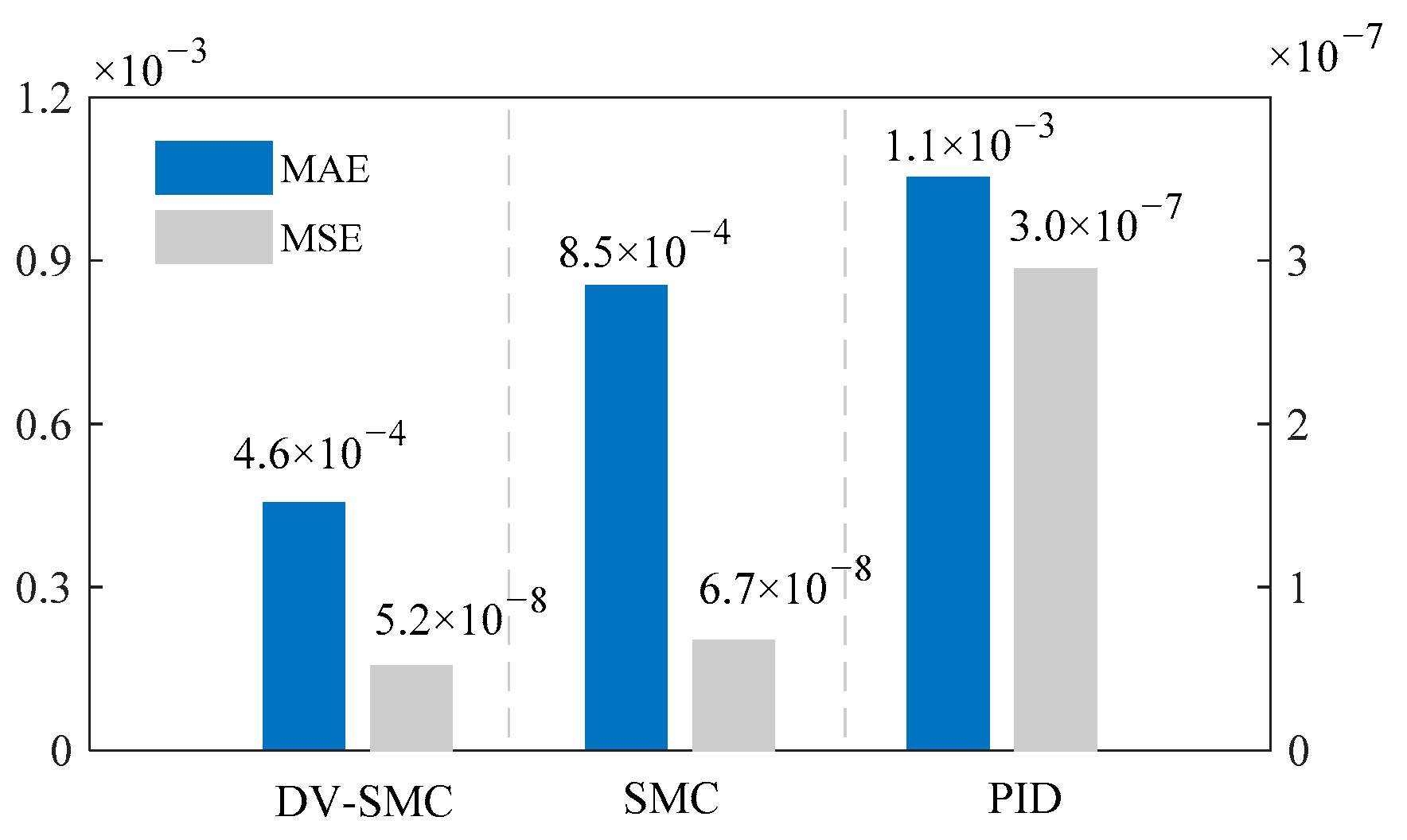
Additionally, Figure 11 shows the outcomes of the sinusoidal tracking test. The SM controller, due to its nonlinear robust compensation, is able to overcome the impact of the dead zone without topping phenomenon. At the point of , the output rise on the SM controller can result in a more stable state of EHA. By contrast, there is a dead-time effect on the PID control output. In spite of the feedforward compensation of and , the DV-SM controller exploits the compensation effect of ESO. According to Figure 11, compared to the SM controller, our model obtains a better tracking result. The maximum absolute errors (MAE), as well as the mean square errors (MSE) of the models, are presented in Figure 12, which confirms the stability of our controller in sinusoidal tracking tasks. The effectiveness of the variable damping strategy, in terms of suppressing overshoot, leads us to conclude that DV-SMC has a more stable step response.
6. Conclusions
In this research, a novel sliding mode control strategy with a damping variable sliding surface, composed of a damping variable sliding mode controller and an extended state observer, was designed and deployed for EHA controlling. Computational modeling and simulations were established to preliminarily analyze the properties of the DV-SMC. In line with the simulation, experimental results revealed that the proposed DV-SMC with double-loop PID control outperformed the other control strategies in the evaluation of both overshoot suppression and settling time. As a result, we came to the following conclusions.
Firstly, in EHA operations, the frequency and damping ratio from the second-order oscillation are assessed on the sliding mode surface of SMC. The parameters of the DV-SMC for EHA controlling were defined, which also paved the way for parameter tuning of SMC.
Secondly, the control strategy simulation verified the system response in comparison to a three-loop PID controller and SMC with double-loop PID controller. Simulation outcomes indicated the effectiveness of the variable damping sliding mode surface in restraining overshoot and oscillation. Moreover, the optimal value range of the damping ratio was determined.
Lastly, we performed an experiment showing the capability of the proposed DV-SMC with double-loop PID control via an EHA working system. Even better working performance in overshoot suppression and settling time was achieved. Our controller can be an optimal approach for catering to the demands of EHA controlling.
Author Contributions
Conceptualization, M.W., Y.F. and D.Z.; methodology, M.W., Y.W. and R.Y.; software, M.W.; validation, Y.W.; formal analysis, Y.F.; investigation, R.Y.; resources, D.Z.; data curation, Y.F. and D.Z.; writing—original draft preparation, M.W.; writing—review and editing, M.W., Y.W., R.Y., Y.F. and D.Z.; visualization, M.W. and R.Y.; supervision, Y.F., D.Z.; project administration, Y.F. All authors have read and agreed to the published version of the manuscript.
Funding
This research is a general project supported by the National Natural Science Foundation of China (No. 61520106010) and the Chinese Civil Aircraft Project (MJ-2017-S49).
Acknowledgments
The authors acknowledge the English review process conducted by MDPI services.
Conflicts of Interest
The authors declare no conflict of interest.
References
- Sarigiannidis, A.G.; Beniakar, M.E.; Kakosimos, P.E.; Kladas, A.G.; Papini, L.; Gerada, C. Fault tolerant design of fractional slot winding permanent magnet aerospace actuator. IEEE Trans. Transport. Electrific. 2016, 2, 380–390. [Google Scholar] [CrossRef]
- Qiao, G.; Liu, G.; Shi, Z.; Wang, Y.; Ma, S.; Lim, T.C. A review of electromechanical actuators for More/All Electric aircraft systems. J. Mech. Eng. Sci. 2018, 232, 4128–4151. [Google Scholar] [CrossRef] [Green Version]
- Staman, K.; Veale, A.J.; Kooij, H. The PREHydrA: A Passive Return, High Force Density, Electro-Hydrostatic Actuator Concept for Wearable Robotics. IEEE Rob. Autom. Lett. 2018, 3, 3569–3574. [Google Scholar] [CrossRef]
- Lee, T.; Lee, D.; Song, B.; Baek, Y.S. Design and Control of a Polycentric Knee ExoskeletonUsing an Electro-Hydraulic Actuator. Sensors 2020, 20, 211. [Google Scholar] [CrossRef] [PubMed] [Green Version]
- Lee, D.; Song, B.; Park, S.Y.; Baek, Y.S. Development and Control of an Electro-Hydraulic Actuator System for an Exoskeleton Robot. Appl. Sci. 2019, 9, 4295. [Google Scholar] [CrossRef] [Green Version]
- Nguyen, H.T.; Trinh, V.C.; Le, T.D. An Adaptive Fast Terminal Sliding Mode Controller of Exercise-Assisted Robotic Arm for Elbow Joint Rehabilitation Featuring Pneumatic Artificial Muscle Actuator. Acutators 2020, 9, 118. [Google Scholar] [CrossRef]
- Miller, T.B. Preliminary Investigation on Battery Sizing Investigation for Thrust Vector Control on Ares I and Ares V Launch Vehicles. February 2011. Available online: https://ntrs.nasa.gov/api/citations/20110007153/downloads/20110007153 (accessed on 22 December 2020).
- Sun, W.; Gao, H.; Yao, B. Adaptive Robust Vibration Control of Full-Car Active Suspensions With Electrohydraulic Actuators. IEEE Trans. Control Syst. Technol. 2013, 21, 2417–2422. [Google Scholar] [CrossRef]
- Shang, Y.; Li, X.; Qian, H.; Wu, S.; Pan, Q.; Huang, L.; Jiao, Z. A Novel Electro Hydrostatic Actuator System with Energy Recovery Module for More Electric Aircraft. IEEE Trans. Ind. Electron. 2020, 67, 2991–2999. [Google Scholar] [CrossRef]
- Ren, G.; Esfandiari, M.; Song, J.; Sepehri, N. Position Control of an Electrohydrostatic Actuator with Tolerance to Internal Leakage. IEEE Trans. Control Syst. Technol. 2016, 24, 2224–2232. [Google Scholar] [CrossRef]
- Maré, J.-C.; Fu, J. Review on signal-by-wire and power-by-wire actuation for more electric aircraft. Chin. J. Aeronaut. 2017, 30, 857–870. [Google Scholar] [CrossRef]
- Guo, Q.; Zhang, Y.; Celler, B.G.; Su, S.W. State-constrained control of single-rod electrohydraulic actuator with parametric uncertainty and load disturbance. IEEE Trans. Control Syst. Technol. 2018, 26, 2242–2249. [Google Scholar] [CrossRef]
- Lee, W.; Li, S.; Han, D.; Sarlioglu, B.; Minav, T.A.; Pietola, M. A Review of Integrated Motor Drive and Wide-Bandgap Power Electronics for High-Performance Electro-Hydrostatic Actuators. IEEE Trans. Transp. Electrification. 2018, 4, 684–693. [Google Scholar] [CrossRef]
- Yao, J.; Yang, G.; Ma, D. Internal Leakage Fault Detection and Tolerant Control of Single-Rod Hydraulic Actuators. Math. Prob. Eng. 2014, 2014, 1–14. [Google Scholar] [CrossRef] [Green Version]
- Yao, Z.; Yao, J.; Yao, F.; Xu, Q.; Xu, M.; Deng, W. Model reference adaptive tracking control for hydraulic servo systems with nonlinear neural-networks. ISA Trans. 2020, 100, 396–404. [Google Scholar] [CrossRef] [PubMed]
- Vassilyev, S.N.; Kudinov, Y.I.; Pashchenko, F.F.; Durgaryan, I.S.; Kelina, A.Y.; Kudinov, I.Y.; Pashchenko, A.F. Intelligent Control Systems and Fuzzy Controllers. II. Trained Fuzzy Controllers, Fuzzy PID Controllers. Autom. Remote Control 2020, 81, 922–934. [Google Scholar] [CrossRef]
- Huang, J.; An, H.; Ma, H.; Wei, Q.; Wang, J. Electro-hydraulic Servo Force Control of Foot Robot Based on Feedback Linearization Sliding Mode Control. In Proceedings of the 13th World Congress on Intelligent Control and Automation (WCICA), Changsha, China, 4–8 July 2018; pp. 1441–1445. [Google Scholar]
- Zhou, M.; Mao, D.; Zhang, M.; Guo, L.; Gong, M. A Hybrid Control with PID–Improved Sliding Mode for Flat-Top of Missile Electromechanical Actuator Systems. Sensors 2018, 18, 4449. [Google Scholar] [CrossRef] [Green Version]
- Yang, R.; Fu, Y.; Zhang, L.; Qi, H.; Han, X.; Fu, J. A Novel Sliding Mode Control Framework for Electrohydrostatic Position Actuation System. Math. Prob. Eng. 2018, 2018, 1–22. [Google Scholar] [CrossRef]
- Cukla, A.R.; Izquierdo, R.C.; Borges, F.A.; Perondi, E.A.; Lorini, F.J. Optimum Cascade Control Tuning of a Hydraulic Actuator Based on Firefly Metaheuristic Algorithm. IEEE Lat. Am. Trans. 2018, 16, 384–390. [Google Scholar] [CrossRef]
- Soon, C.C.; Ghazali, R.; Jaafar, H.I.; Hussien, S.Y.S. Sliding Mode Controller Design with Optimized PID Sliding Surface Using Particle Swarm Algorithm. Procedia Comput. Sci. 2017, 105, 235–239. [Google Scholar] [CrossRef]
- Alemu, A.E.; Fu, Y. Sliding Mode Control of Electro-Hydrostatic Actuator Based on Extended State Observer. In Proceedings of the 29th Chinese Control And Decision Conference (CCDC), Chongqing, China, 28–30 May 2017; pp. 758–763. [Google Scholar]
- Bernardes, T.; Montagner, V.F.; Gründling, H.A.; Pinheiro, H. Discrete-Time Sliding Mode Observer for Sensorless Vector Control of Permanent Magnet Synchronous Machine. IEEE Trans. Ind. Electron. 2014, 61, 1679–1691. [Google Scholar] [CrossRef]
- Li, C.; Kang, Z. Synchronization Control of Complex Network Based on Extended Observer and Sliding Mode Control. IEEE Access 2020, 8, 77336–77344. [Google Scholar]
- Nguyen, V.-C.; Vo, A.-T.; Kang, H.-J. A Non-Singular Fast Terminal Sliding Mode Control Based on Third-Order Sliding Mode Observer for a Class of Second-Order Uncertain Nonlinear Systems and Its Application to Robot Manipulators. IEEE Access 2020, 8, 78109–78120. [Google Scholar] [CrossRef]
- Gao, X.; Ren, Z.; Zhai, L.; Jia, Q.; Liu, H. Two-Stage Switching Hybrid Control Method Based on Improved PSO for Planar Three-Link Under-Actuated Manipulator. IEEE Access 2019, 7, 76263–76273. [Google Scholar] [CrossRef]
- Ren, H.-P.; Zhou, R. Fuzzy Sliding Mode Tracking Control for DC Motor Servo System without Uncertainty Information. In Proceedings of the 12th IEEE Conference on Industrial Electronics and Applications (ICIEA), Siem Reap, Cambodia, 18–20 June 2017; pp. 1511–1521. [Google Scholar]
- Parseihian, G.; Gondre, C.; Aramaki, M.; Ystad, S.; Kronland-Martinet, R. Comparison and Evaluation of Sonification Strategies for Guidance Tasks. IEEE Trans. Multimedia 2016, 18, 674–686. [Google Scholar] [CrossRef] [Green Version]
- Kota, I.; Umeda, K.; Tsuda, K.; Sakaino, S.; Tsuji, T. Force Control of Electro-Hydrostatic Actuator Using Pressure Control Considering Torque Efficiency. In Proceedings of the IEEE 15th International Workshop on Advanced Motion Control (AMC), Tokyo, Japan, 9–11 March 2018; pp. 385–390. [Google Scholar]
- Zhang, J.; Liu, X.; Xia, Y.; Zuo, Z.; Wang, Y. Disturbance observer-based integral sliding-mode control for systems with mismatched disturbances. IEEE Trans. Ind. Electron. 2016, 63, 7041–7047. [Google Scholar] [CrossRef]
- Zhou, L.; Che, Z.; Yang, C. Disturbance Observer-Based Integral Sliding Mode Control for Singularly Perturbed Systems with Mismatched Disturbances. IEEE Access 2018, 6, 9854–9861. [Google Scholar] [CrossRef]
- Wang, X.; Li, S.; Yu, X.; Yang, J. Distributed Active Anti-Disturbance Consensus for Leader-Follower Higher-Order Multi-Agent Systems with Mismatched Disturbances. IEEE Trans. Autom. Control 2017, 62, 5795–5801. [Google Scholar] [CrossRef]
- Utkin, V. Variable structure systems with sliding modes. IEEE Trans. Autom. Control 1977, 22, 212–222. [Google Scholar] [CrossRef]
- Din, S.U.; Khan, Q.; Fazal, U.-R.; Akmeliawanti, R. A comparative experimental study of robust sliding mode control strategies for underactuated systems. IEEE Access 2017, 5, 10068–10080. [Google Scholar] [CrossRef]
- Castanos, F.; Fridman, L. Analysis and design of integral sliding manifolds for systems with unmatched perturbations. IEEE Trans. Autom. Control 2006, 51, 853–858. [Google Scholar] [CrossRef] [Green Version]
- Estrada, A.; Fridman, L. Quasi-continuous hosm control for systems with unmatched perturbations. Automatica 2010, 46, 1916–1919. [Google Scholar] [CrossRef]
- Stojic, M.; Siljak, D. Generalization of Hurwitz, Nyquist, and Mikhailov stability criteria. IEEE Trans. Autom. Control 2003, 10, 250–254. [Google Scholar] [CrossRef]
- Mujumdar, A.; Tamhane, B.; Kurode, S. Observer-Based Sliding Mode Control for a Class of Noncommensurate Fractional-Order Systems. IEEE/ASME Trans. Mechatron. 2015, 20, 2504–2512. [Google Scholar] [CrossRef]
- Wimatra, A.; Sunardi; Margolang, J.; Sutrisno, E.; Nasution, D.; Suherman; Turnip, A. Active suspension system based on Lyapunov method and ground-hook reference model. In Proceedings of the 2015 International Conference on Automation, Cognitive Science, Optics, Micro Electro-Mechanical System, and Information Technology (ICACOMIT), Bandung, Indonesia, 29–30 October 2015; pp. 101–105. [Google Scholar]
Figure 1.
Schematic diagram of an electro-hydrostatic actuator (EHA).

Figure 2.
Damping ratio changing along with error and sensitivity factor.

Figure 3.
Block diagram of cascade control structure.

Figure 4.
Simulation response to different reference inputs.

Figure 5.
System response with different .

Figure 6.
Schematic of test rig.

Figure 7.
Response to different reference input.

Figure 8.
Overshoot of different control strategies.

Figure 9.
Settling time of different control strategies. 1+ in Figure 9 represents that the settling time of SMC and PID on the 5 mm step input is longer than the signal collecting time (1s).
Figure 9.
Settling time of different control strategies. 1+ in Figure 9 represents that the settling time of SMC and PID on the 5 mm step input is longer than the signal collecting time (1s).

Figure 10.
Control output of different reference inputs.

Figure 11.
Sinusoidal tracking outcomes.

Figure 12.
Tracking error of different controllers.


Table 1.
Specifications for simulation initialization.
| Parameter | Value |
|---|---|
| Piston effective area | |
| Effective stroke | |
| Leakage coefficient | |
| Fluid elastic modulus | |
| Hydraulic cylinder volume | |
| Cylinder viscous friction | |
| Mass of cylinder and load | |
| Pump displacement | |
| Motor viscous friction | |
| Phase resistance | |
| Phase inductance | |
| Motor spindle moment of inertia | |
| Torque coefficient | |
| Back EMF coefficient | |
| Elastic load coefficient | |
| Bus voltage |
Table 2.
Specifications of EHA.
| Parameter | Value |
|---|---|
| Rated pressure | |
| Rated speed | |
| Rated force | |
| Effective displacement | |
| Rated power supply | |
| Bandwidth |
Publisher’s Note: MDPI stays neutral with regard to jurisdictional claims in published maps and institutional affiliations. |
© 2020 by the authors. Licensee MDPI, Basel, Switzerland. This article is an open access article distributed under the terms and conditions of the Creative Commons Attribution (CC BY) license (http://creativecommons.org/licenses/by/4.0/).
Share and Cite
MDPI and ACS Style
Wang, M.; Wang, Y.; Yang, R.; Fu, Y.; Zhu, D. A Sliding Mode Control Strategy for an ElectroHydrostatic Actuator with Damping Variable Sliding Surface. Actuators 2021, 10, 3. https://0-doi-org.brum.beds.ac.uk/10.3390/act10010003
AMA Style
Wang M, Wang Y, Yang R, Fu Y, Zhu D. A Sliding Mode Control Strategy for an ElectroHydrostatic Actuator with Damping Variable Sliding Surface. Actuators. 2021; 10(1):3. https://0-doi-org.brum.beds.ac.uk/10.3390/act10010003
Chicago/Turabian StyleWang, Mingkang, Yan Wang, Rongrong Yang, Yongling Fu, and Deming Zhu. 2021. "A Sliding Mode Control Strategy for an ElectroHydrostatic Actuator with Damping Variable Sliding Surface" Actuators 10, no. 1: 3. https://0-doi-org.brum.beds.ac.uk/10.3390/act10010003
Note that from the first issue of 2016, this journal uses article numbers instead of page numbers. See further details here.