The Novel Singular-Perturbation-Based Adaptive Control with σ-Modification for Cable Driven System


1
School of Automation Science and Electrical Engineering, Beihang University, Beijing 100191, China
2
Ningbo Institute of Technology, Beihang University, Ningbo 315800, China
3
Department of Electrical and Electronic Engineering, University of Nottingham, Nottingham NG7 2RD, UK
*
Author to whom correspondence should be addressed.
Actuators 2021, 10(3), 45; https://0-doi-org.brum.beds.ac.uk/10.3390/act10030045
Submission received: 1 February 2021
/
Revised: 9 February 2021
/
Accepted: 11 February 2021
/
Published: 28 February 2021
(This article belongs to the Section Precision Actuators)
Abstract
:Due to their large working space and fast response, cable driven systems have been widely applied in manufacturing, robotics and motion simulators, etc. However, the cable is flexible and tends to resonate at high frequencies, which raises challenges for the motion control of the cable driven system. To solve this problem, this paper proposes a singular-perturbation-based adaptive control method with -modification. Taking advantage of the multi-time scale characteristics, the flexible system is approximately decomposed into two subsystems, and then the damping compensation is designed in the boundary layer subsystem to enhance the tension stability. In addition, estimated parameters drift may occur for the reduced-order system. Thus, the -modification is proposed to ensure that the tracking and estimation errors converge to a bounded residual set. The Lyapunov stability theorem proves that the closed-loop system is stable and errors are ultimately uniformly bounded. A research prototype of a twin-motor cable driven system is developed, and experimental investigation is conducted on it. The experimental results show that the proposed control method can effectively suppress cable resonance at high frequencies. Compared with the conventional adaptive control method, it can significantly increase the system bandwidth.
1. Introduction
Cable driven systems have been widely used in lifting [1,2], telescopes [3], robotics [4,5], motion simulators [6,7] and other fields [8,9]. Different from a rigid transmission system, it has two inherent properties [5,10]: (1) the cable can only be pulled but not pressed, so redundant actuation must be adopted to make the end effector fully controllable; (2) the cable is elastic. At high frequencies, resonance often occurs, which severely affects the performance and stability of the system and brings great challenges to the system control. In existing literature, internal tension compensation is used to solve the problem of unidirectional force, and the motion control is achieved by treating the cable driven system as a rigid system [11,12,13]. Typical methods include the computed torque control method [14,15,16] and robust adaptive control method [17,18,19,20,21,22,23].
Inspired by the feedback linearization theory, Alp et al. [24] proposed a computed torque method based on the nominal model for the position control of a suspended robot, and proved the stability of the system. However, due to the parameter uncertainty in the system, the control performance is greatly compromised. To solve this problem, robust adaptive control is one good solution. To reduce the negative effect of dynamic parameters uncertainty, Li et al. [18] proposed a robust adaptive control, by adding online estimation of dynamic parameters. Wang et al. [19] proposed a time-delay estimation method, and combined it with terminal sliding mode control to achieve an adaptive integral terminal sliding mode control for cable-driven manipulators. Moreover, Wang et al. [20] introduced the super-twisting algorithm into the adaptive control scheme to ensure that the system can reach the sliding mode surface in limited time. Shang et al. [17] also conducted an in-depth study on the sliding mode control of the cable driven system. They combined the second-order sliding mode control with the synchronization control, and proposed a compound robust control with high precision and robustness. To further improve the control accuracy, Shang et al. [25] introduced the cross-coupled control and parameters adaptive compensation to the synchronization control, and then proposed an adaptive cross-coupled control scheme. Lamaury et al. [26] further extended the adaptive control to the workspace and joint space, and proposed a dual-space adaptive control strategy. The above studies are mainly on the motion control of systems in low dynamics. Because the high frequency characteristics of the cable are filtered, these control methods based on the rigid model can also perform well for the flexible systems.
However, for systems in high dynamic motion, the filtering effect weakens significantly. Thus, it is not equivalent to a rigid system anymore. Specifically, by considering the cable flexibility, the system is converted to a series-connected dual-mass system from a single-mass system. The controller based on a rigid model cannot guarantee the full state stability of a flexible system, especially the cable tension that easily becomes unstable due to insufficient cable damping. This problem has aroused the attention of researchers [27]. Khosravi et al. proposed the cascade control method to keep the tension stable by employing the internal tension control of the cable to avoid tension drift [28,29,30]. Theoretically, this method is feasible. However, it is difficult to collect high-quality tension signals, which affects the tension control. Furthermore, the dual closed loops in the cascade control is quite challenging. This method is poor to implement, especially for high-dynamics motion, a simpler controller is better, and cascade control contradicts this requirement. To solve this problem, the singular perturbation control was proposed [31,32]. The multi-time scales of the flexible system are employed to decompose the system into two subsystems, i.e., the boundary layer and the reduced-order system, and the damping compensation is designed in the boundary layer to keep the tension stable. Compared with the cascade controller, this method is simpler and more practical, and force sensors are not required in the system design.
However, so far the control algorithms of cable driven systems have not considered the drift of estimation parameters, which unavoidably compromises the motion control performance especially in high dynamics. Therefore, this paper proposed a singular-perturbation-based adaptive control with -modification to avoid the parameter drift instability, and to give the sufficient conditions for the system stability.
The main contributions of the paper are as follows.
- (1)
- Based on the singular perturbation theory, an adaptive control method with -modified adaptive law is proposed.
- (2)
- The stability of the flexible system is proved theoretically, and sufficient conditions for system stability are given.
- (3)
- This method is the first time to be used for the control of a flexible system with high-frequency motion.
- (4)
- The effectiveness of the proposed method is validated by experiments.
The rest is organized as follows. In Section 2, the schematic structure of the twin-motor cable driven system, a typical cable driven parallel mechanism, is introduced, and kinematics and dynamics models are formulated analytically. In Section 3, based on the singular perturbation theory, an adaptive composite control with -modification is proposed. In Section 4, the stability of the closed-loop system is proved, and sufficient conditions for the flexible system are given. In Section 5, the developed twin-motor cable driven system is presented, and an experiments are conducted. The experimental results are utilized to validate the proposed control method. Finally, the research work is concluded in Section 5.
2. Analysis of Flexible System Kinematics and Dynamics
2.1. System Architecture
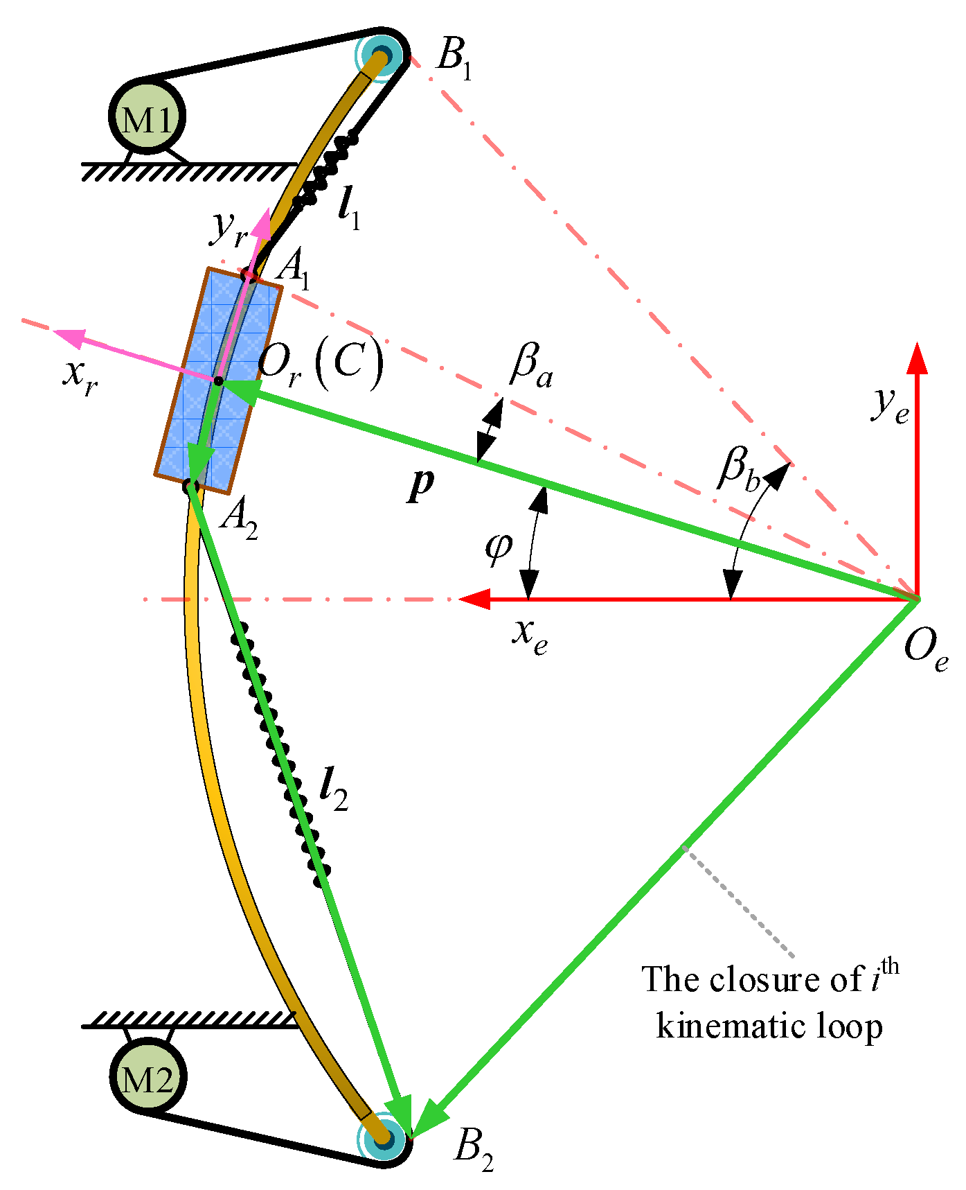
The studied twin-motor cable driven system is shown in Figure 1. It is composed of motors, an arc guide rail, flexible cable, pulleys and the moving platform. Affected by the unidirectional force property of the flexible cable, the moving platform can only reciprocate along the arc guide under the cooperative traction of the motors on both sides. This system is a typical redundant actuation system. To facilitate subsequent discussion, the fixed coordinate system E: () on the base frame and the reference coordinate system R: () on the moving platform are set, and their origins and are coincident with the arc center and the centroid of the moving platform, respectively.
2.2. Analysis of System Kinematics
The vector of the ith cable is represented as
where denotes the cable length between points and , the unit vector of cable tension, the position vector of point , the position vector of point , the position vector of the origin and the rotation matrix of frame with respect to frame .
From (1), the velocity mapping between the cable length and the end effector is
where , denotes the angle between and the positive , and
denotes the radius of the guide rail, the angle between the cable tension and the positive and the structure parameter as shown in Figure 1.
It is worth noting that, affected by the elasticity of the cable, the speeds of the two ends of the same cable are different, and they meet the following conditions
where denotes the cable velocity at points , the cable velocity at motor connection, , the motor rotation angle and the radius of the winch,
2.3. Analysis of System Dynamics
2.3.1. Dynamics Model
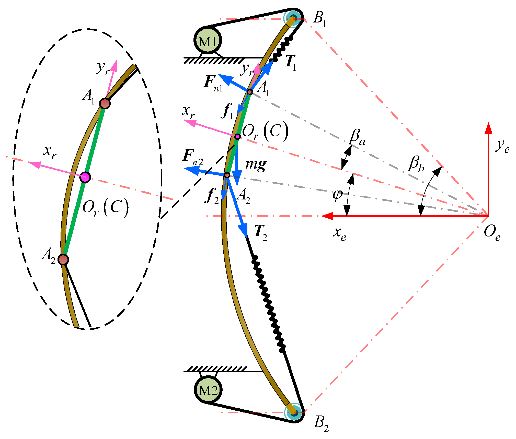
The force is shown in Figure 2. According to the theorem of momentum, the dynamics of the moving platform is
where denotes the vector of the centroid of platform, m the platform mass, the acceleration vector of the center of mass, the moment of inertia of the platform about the centroid of mass, the rotational acceleration, the position vector of point , the tension vector, the gravity acceleration, and the friction vector
is the viscosity coefficient and is the coulomb friction.
In (7), the cable tensions are
where denotes the cable stiffness, and the movement displacement of cables at motor and points , respectively. The dynamics of motors is
where denotes the inertia matrix, the radius of the winch, the motor torque.
2.3.2. Dynamics Model Analysis
In (11) and (12), the stiffness is much larger than other parameters. To facilitate analysis, define
where is a small positive parameter, is on the order of 1 and is the unit matrix. Substituting (9) and (14) into (12), the dynamics of the motor can be rewritten as
Since is much smaller than other parameters, the changing rate of tension in (15) far exceeds that of q in (11). On the time scale, the variables and q can be divided into two types: fast and slow. When the fast variable changes, the slow variable q can be considered frozen. Therefore, in (15), the transfer function from the torque to the cable tension can be approximated as a second-order system. At low frequencies, due to the filtering of the system itself, the high-frequency part of the system response is filtered, and the flexible system is equivalent to a rigid one. As the frequency increases, the system’s ability to filter high-frequency response decreases, and the impact of the flexible cable on the system gradually increases. When a certain frequency is reached, the impact of the flexible cable cannot be ignored, and even damage the system stability. To solve this problem, a composite adaptive control scheme based on singular perturbation is proposed.
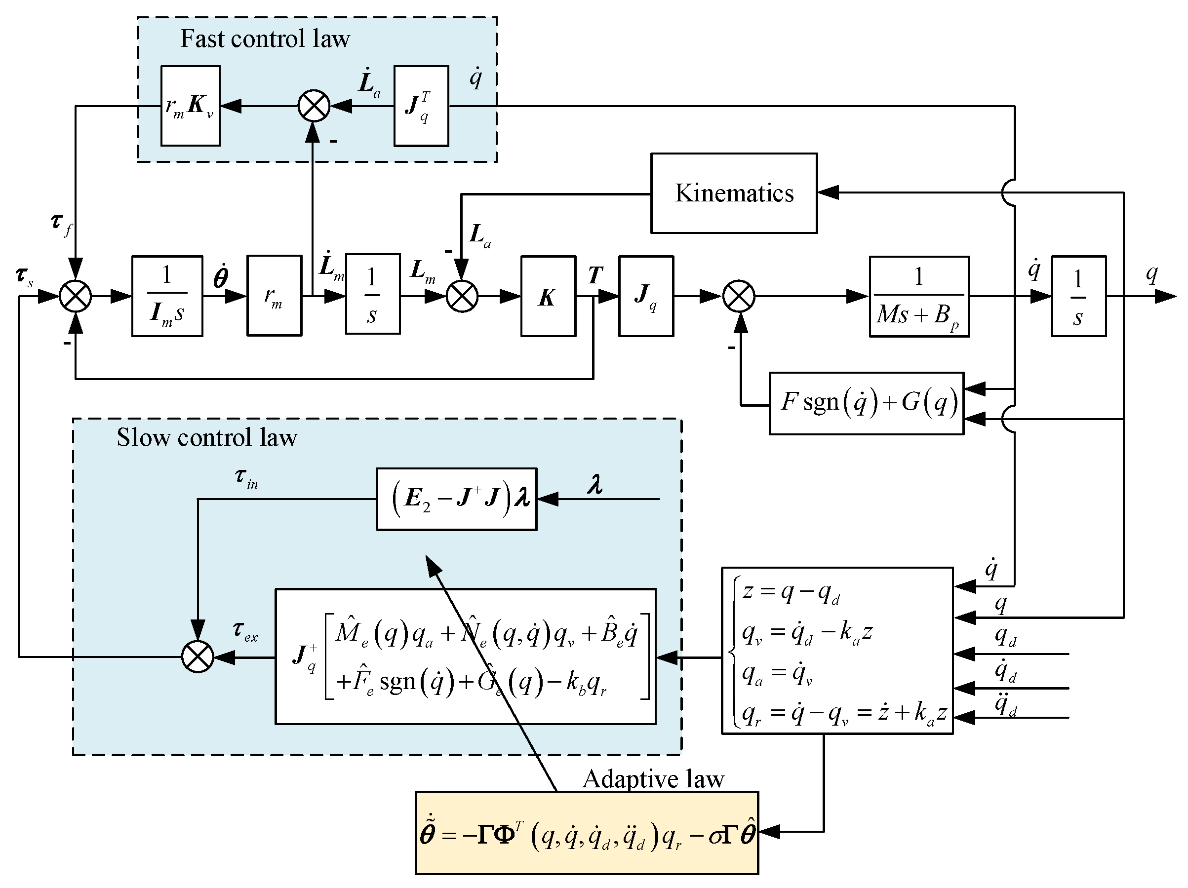
3. Composite Control Scheme
Since the system has multiple time scales, the system can be divided into fast (boundary layer) and slow (reduced-order) subsystems, and then the control laws are designed for each subsystem to form the composite control law, i.e.,
where denotes the slow control law, the fast control law and the feedback gains. Define
where is on the order of 1. Substituting (16) into (15), the system can be written as
Moreover, from (19), it can be seen that the stability of the fast variable can be improved by the compensation of fast control law without any impact on the reduced-order system. When , both (15) and (19) can be degenerated into the same reduced-order model as the rigid model.
where
Therefore, the control schemes for the rigid system still work for the reduced-order system. Considering the uncertainty of dynamic parameters, the slow control law is designed as
where and denote the effective force and internal force, respectively, the estimated parameter, the pseudo-inverse and any 2-dimensional column vector,
is the desired trajectory, and are the adjustable gains. Then combining (20) and (22)–(25) gives the closed-loop dynamics of the reduced-order system
where
To prevent the estimated parameters from drifting, the adaptive law is designed as
where is the gain matrix, a positive constant. According to the above, the designed composite adaptive controller is shown in Figure 3.
4. Stability Analysis
Based on the singular perturbation theory and Lyapunov’s stability theorem, the stability of a close-loop system is analyzed. It includes four parts: singular perturbation standardization, boundary layer stability analysis, reduced-order system stability analysis, and overall system stability analysis.
4.1. Singular Perturbation Standardization
Define the slow, fast and intermediate variables as
Then from (11) and (19), the standard singular perturbation model of the closed loop is
where
See Appendix A for the detailed derivation. When , the isolated root of is
where is the quasi-steady state of . However, due to the difference of the initial conditions and perturbation of , deviates from the actual . The deviation is defined as
Substituting (37) into (33) and (34), and combining with (29), the standard singular perturbation model is rewritten as
where .
4.2. Boundary Layer and Stability Analysis
Define the fast-time scale , then (38)-3 can be represented as
From the above formula, the boundary layer is
where is a Hurwitz matrix that can be achieved by adjusting the gains and . Then for any given positive definite matrix , there exists a unique positive definite matrix that satisfies
Then for the boundary layer, choose the Lyapunov function candidate as
Along the boundary layer system , the fast-time derivative of is
where denotes the smallest eigenvalue of matrix . Hence, as presented in (42) and (43), for all , and , i.e., when , and the boundary layer is asymptotically stable.
4.3. Reduced-Order System and Stability Analysis
From (38), the reduced-order model of flexible system is obtained as
Then for the reduced-order system, choose the Lyapunov function candidate as
where . Along the reduced-order system , the time derivative of is
where ,
can be kept positive definite by adjustment of and . Define the sets:
Hence, as presented in (45) and (46), for all , and , i.e., will convergence to the residual set , and the reduced-order system is stable.
4.4. Stability Analysis of the Flexible System
According to the above two Lyapunov functions, the following composite Lyapunov function candidate for the flexible system is chosen as
where d is constant parameter. Then along the original flexible system S, the time derivate of V is
Note that the first two terms in (51) are the time derivatives of and with respect to the reduced-order system and the boundary layer, respectively. From (43) and (46) we know that they are stable. The remaining two items are the interconnection between the slow/fast subsystem and the original system. Combining (38), (44) and (45) gives
where . Combining (38), (40) and (42) gives
where is defined in (41).
Theorem 1.
For continuous and bounded , there exists positive constants and positive function satisfying
Proof of Theorem 1.
See Appendix B. □
Substituting (54) into (53), we get
where, , , , . Hence, substituting (43), (46), (52) and (55) into (51), we get
where,
When
is a positive definite matrix, which can be easily achieved by adjusting d in this system. Then define the following sets
where , .
Therefore, according to (56), for all , can be positive or negative, but for all , definitely. It means that for all , they either converge or diverge, but once they exceed the set , will remove towards the origin and converge to the set again. The singular-perturbation-based adaptive control with -modification method avoids the drift of estimated parameters, and enables all errors to converge to a residual set. The closed-loop of the flexible system is stable.
5. Experimental Validation
5.1. Experimental Setup
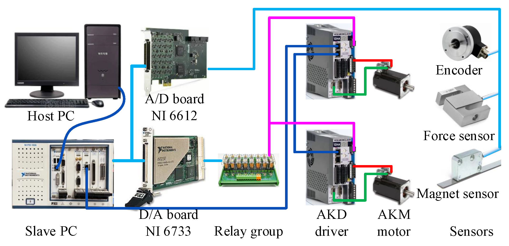
One research prototype of the twin-motor cable driven system is developed as shown in Figure 4. It is mainly composed of two parts: the transmission system and the control system. The transmission system includes motors, cables, an arranging mechanism, a guide rail and sensors. Cables are connected between the motors and the moving platform. To prevent cables from winding irregularly, the cable arrangement mechanism is also designed and installed on each motor, so that the cables can be arranged on the rotating shaft regularly.
The measurement and control system is shown in Figure 5, the hardware includes the host and slave computers, A/D and D/A boards, drivers, motors and sensors. Based on the Labview software, the control program is designed with functions of command input, status detection, data processing and storage. All data in the slave computer will be processed within 1 ms. Therefore, the applicability of the control method should be considered.
Experiments are conducted on the test bed to validate the proposed composite adaptive control with -modification (-CAC), and compare with the traditional adaptive control algorithm (TAC). Specifically, it is to verify that the proposed method helps to improve the bandwidth of the cable driven system. The parameters of the two controllers are listed in Table 1.
5.2. Experimental Results and Discussion
The tracking command is
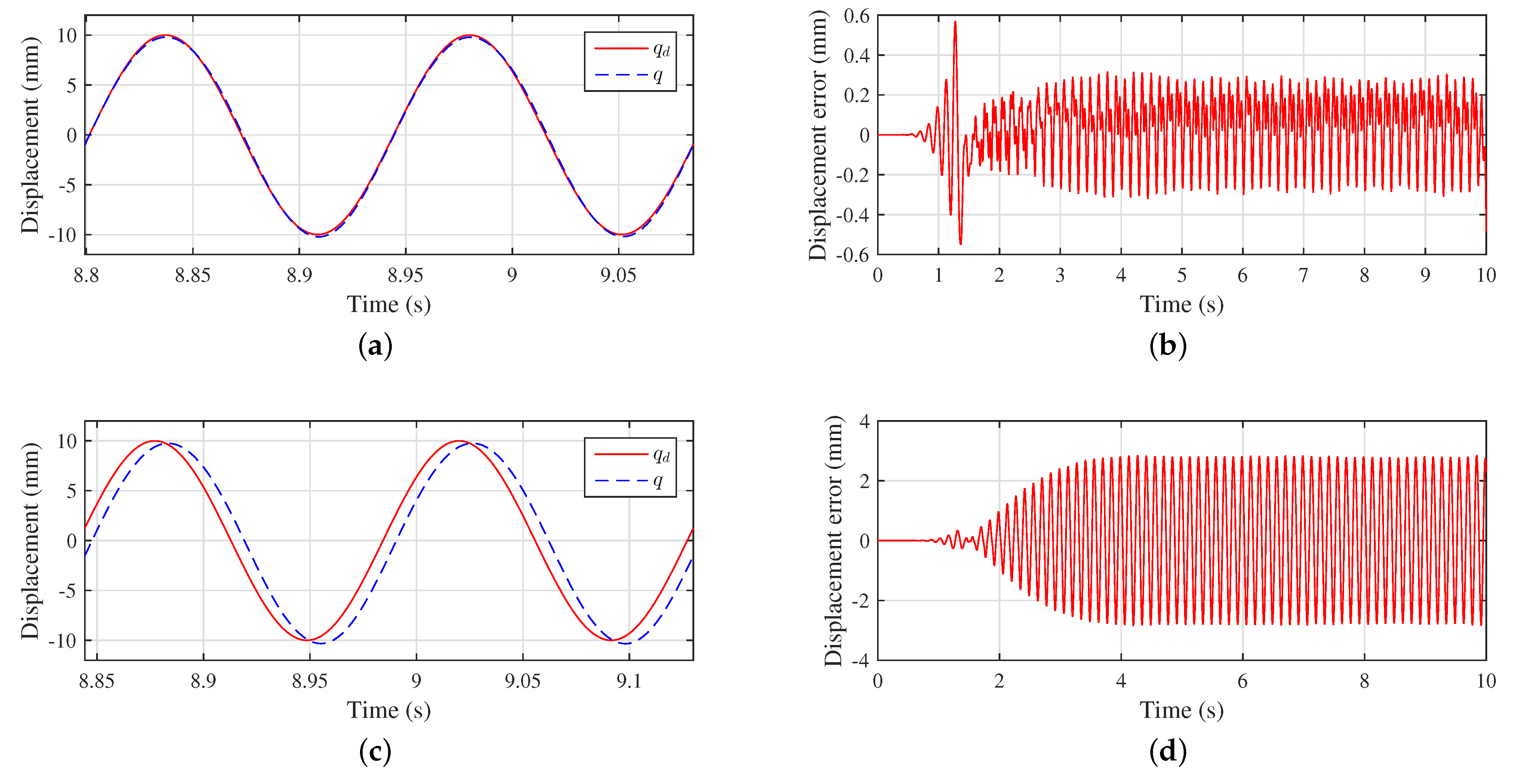
where denotes the amplitude, and the frequency. The amplitude is fixed at 10 mm, and experiments with frequencies of 2∼9 Hz have been done, respectively. As shown in Figure 6, both TAC and -CAC perform well at 3 Hz, except for the start-up phase. They both can keep the tracking error within ±1mm. However, because of the compensation of the fast control law in the -TCT, it has a stronger control effect and further reduces the error within ±0.5 mm. The high-frequency characteristics of the flexible cable show little effect at 3 Hz.
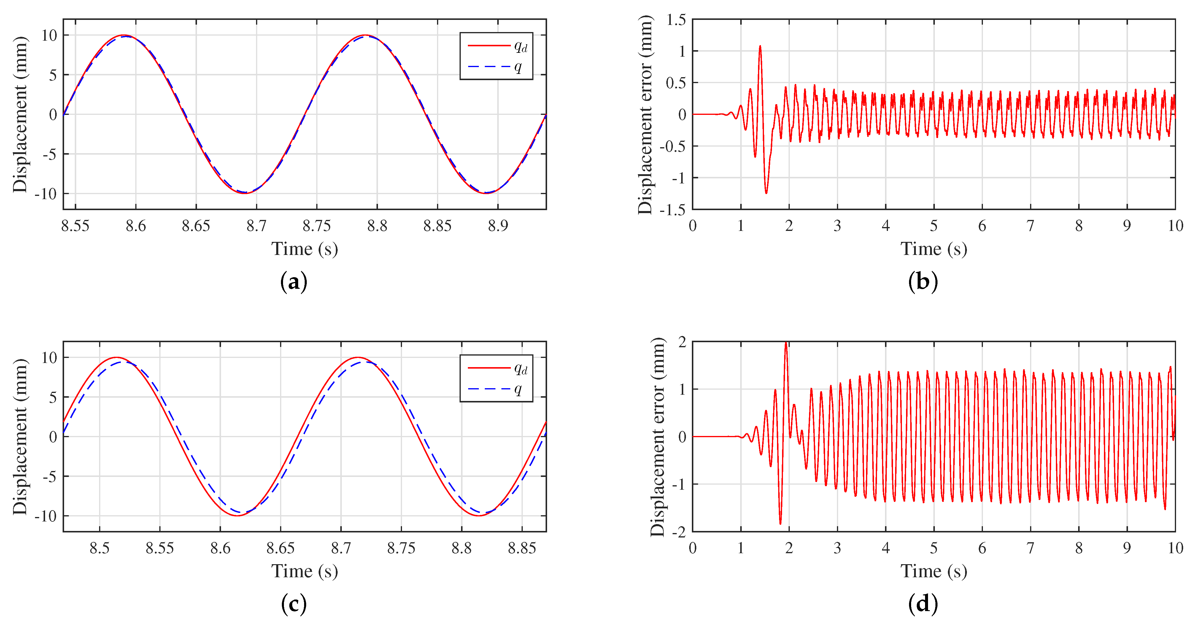
The frequency is further increased to 5 Hz, as shown in Figure 7. Compared with 3 Hz, the performance of the TAC deteriorates. Specifically, the tracking error increases from ±1 to ±1.5 mm, and the phase lags obviously. While the -CAC continues to maintain high accuracy, its error is kept within ±0.5 mm, and phase follows closely. The -CAC shows advantage at 5 Hz.
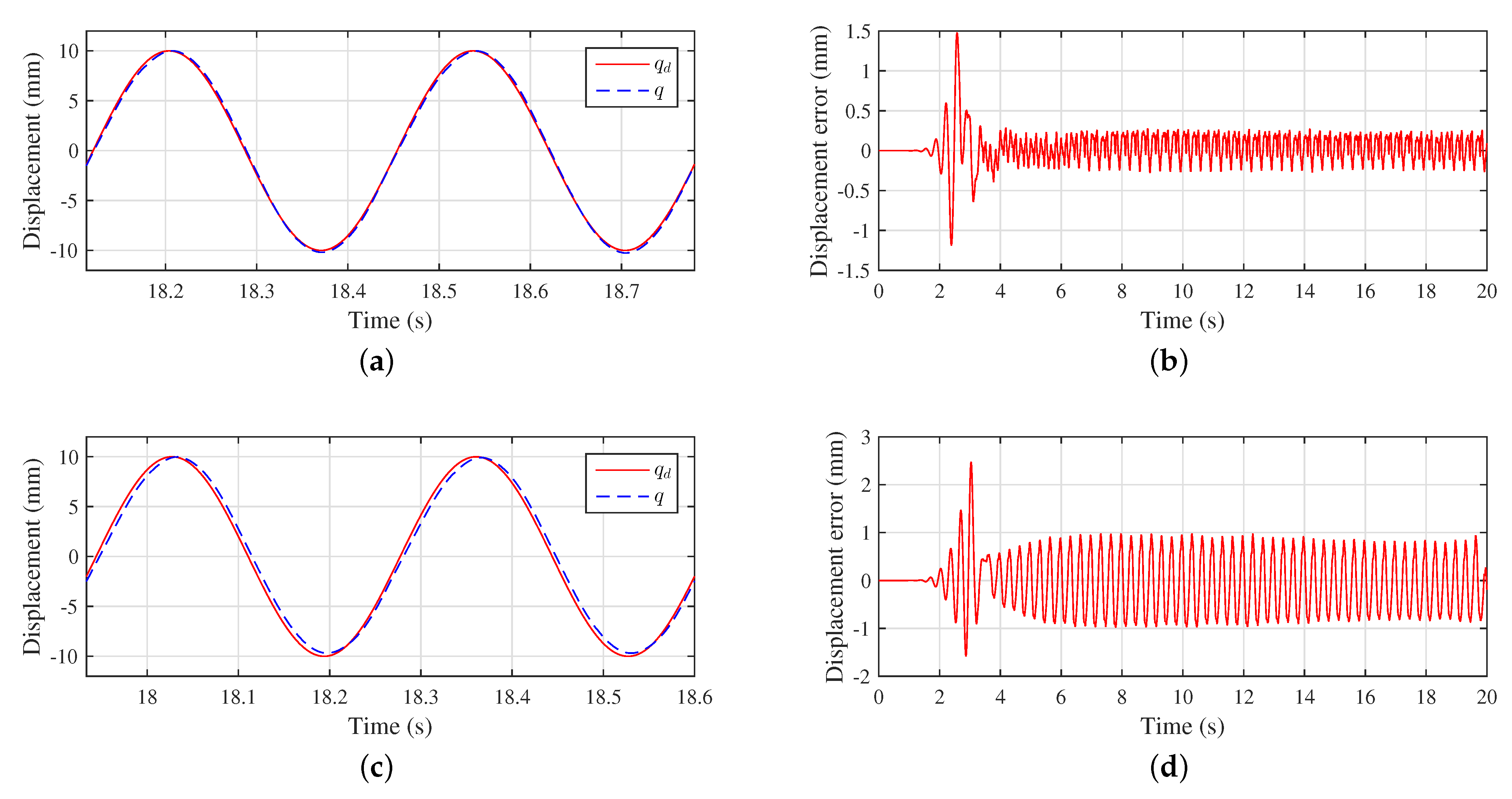
The frequency is increased to 7 Hz again, as shown in Figure 8. Compared with 3 and 5 Hz, the performance of the TAC gets worse as the frequency increases. The tracking error increases from the initial ±1 to ±3 mm, and there is a serious phase lag. The -CAC showed consistency in 3, 5, and 7 Hz experiments. This consistency is the evidence that the -CAC can make the flexible system more stable. Compared with TAC, the -CAC significantly improves the performance at 7 Hz.
The detailed comparison results of the two controllers in the frequency domain are recorded in Table 2. It shows that as the frequency increases, their performance deteriorates. However, the deterioration rate of the -CAC is much slower than the TAC. At 9 Hz, the -CAC can still ensure that the phase lag of system is less than 10 degrees and the amplitude error does not exceed 10%, while, the TAC is already worse than this performance at 6 Hz. The -CAC successfully increases the system bandwidth from 5 to 9 Hz. As shown in Figure 9, at 9 Hz, the -CAC can still work stably, and the phase lag is about −9.2 degrees.
The above comparative results consistently show that with the increase of the frequency, the influence of the flexible characteristics of the cable on the system control increases. At low frequencies that far away from the cable characteristics, TAC and -CAC both perform well. However, at high frequencies, the TAC performs poorly for the cable flexibility. While, the -CAC, due to the fast control law compensation, can effectively weaken the flexible cable influence. Hence, the -CAC shows obvious advantages in the high-frequency experiments. Figure 6, Figure 7 and Figure 8 and Table 2 directly show that the -CAC is significantly effective for increasing the bandwidth of the flexible system.
6. Conclusions
Based on the singular perturbation theory, a -modified adaptive control algorithm has been proposed to solve the control of a twin-motor cable driven system. The special feature of this method is that it uses the multi-time scale characteristics of the system to design a composite control law, which can be divided into fast and slow parts. In addition, to prevent instability of estimated parameters drift, a -modification was applied to the adaptive law. Then, stability was proved by the Lyapunov stability theorem. Results show that the closed-loop of the flexible system is stable, and all errors converge into a residual set. One research prototype of the twin-motor cable driven system has been developed, and experimental investigation was conducted on both the proposed -modified adaptive control method and conventional adaptive control method. The comparison of experimental results show that the proposed -modified adaptive control method can improve the tracking performance well, especially for high-frequency motion control, the fast control law compensation effectively reduces the risk of internal tension instability and enables the system to be stable with large control gains. The proposed -modified adaptive control algorithm successfully increases the system bandwidth from 5 Hz in the traditional adaptive control algorithm to 9 Hz.
Author Contributions
Conceptualization, B.L. and L.Y.; methodology, B.L. and L.Y.; software, B.L.; validation, B.L. and L.Y.; formal analysis, B.L.; investigation, B.L.; resources, B.L.; data curation, B.L.; writing—original draft preparation, B.L.; writing—review and editing, B.L., L.Y. and C.G.; visualization, B.L.; supervision, L.Y.; project administration, L.Y.; funding acquisition, L.Y. All authors have read and agreed to the published version of the manuscript.
Funding
This research was funded by the National Natural Science Foundation of China (NSFC) under grant 51875013, the Major Project of Ningbo Science and Technology Innovation 2025 Program under grant 2019B10071, the Major Project of the New Generation of Artificial Intelligence under grant 2018AAA0102900, the National Key R&D Program of China under grant 2017YFB1300400, and Fundamental Research Funds for the Central Universities.
Institutional Review Board Statement
Not applicable.
Informed Consent Statement
Not applicable.
Data Availability Statement
Data available on request due to restrictions eg privacy or ethical.
Acknowledgments
The authors are thankful for the support of the Science and Technology on Aircraft Control Laboratory and Research Institute for Frontier Science, Beihang University, Beijing 100191, China.
Conflicts of Interest
The authors declare no conflict of interest.
Abbreviations
The following abbreviations are used in this manuscript:
| -CAC | composite adaptive control with -modification |
| TAC | traditional adaptive control |
Appendix A
Appendix B
Recall the defined in (32) and expand it as
Combining (11) and (A8) gives
Then define
Equation (A9) can be rewritten as
Substituting the slow control law (22) into (A11) gives
that is,
Hence the time derivative of is
where
Combining (A14) with (38) gives
From (A16), there exist corollaries satisfying
- Corollary 1
- Corollary 2
- Corollary 3
References
- Shiang, W.J.; Cannon, D.; Gorman, J. Dynamic analysis of the cable array robotic crane. In Proceedings of the 1999 IEEE International Conference on Robotics and Automation, Detroit, MI, USA, 10–15 May 1999; pp. 2495–2500. [Google Scholar] [CrossRef]
- Vrabel, R. Design of the state feedback-based feed-forward controller asymptotically stabilizing the double-pendulum-type overhead cranes with time-varying hoisting rope length. Int. J. Nonlinear Sci. Numer. Simul. 2020, 1–12. [Google Scholar] [CrossRef]
- Nan, R.; Li, D.; Jin, C.; Wang, Q.; Zhu, L.; Zhu, W.; Zhang, H.; Yue, Y.; Qian, L. The five-hundred-meter aperture spherical radio telescope (FAST) project. Int. J. Mod. Phys. D 2011, 20, 989–1024. [Google Scholar] [CrossRef] [Green Version]
- Pott, A.; Mütherich, H.; Kraus, W.; Schmidt, V.; Miermeister, P.; Verl, A. IPAnema: A family of Cable-Driven Parallel Robots for Industrial Applications. In Cable-Driven Parallel Robots, 1st ed.; Bruckmann, T., Pott, A., Eds.; Springer: Berlin/Heidelberg, Germany, 2013; Volume 12, pp. 119–134. [Google Scholar]
- Wang, Y.; Song, C.; Zheng, T.; Lau, D.; Yang, K.; Yang, G. Cable Routing Design and Performance Evaluation for Multi-link Cable-Driven Robots with Minimal Number of Actuating Cables. IEEE Access 2019, 7, 135790–135800. [Google Scholar] [CrossRef]
- Lachele, P.M.; Boss, R. The cablerobot simulator large scale motion platform based on cable robot technology. In Proceedings of the 2016 IEEE/RSJ International Conference on Intelligent Robots and Systems (IROS), Daejeon, Korea, 9–14 October 2016; pp. 3024–3029. [Google Scholar] [CrossRef]
- Tadokoro, S.; Murao, Y.; Hiller, M.; Murata, R.; Matsushima, T. A motion base with 6-DOF by parallel cable drive architecture. IEEE-ASME Trans. Mechatron. 2002, 7, 115–123. [Google Scholar] [CrossRef]
- Lee, T.; Kim, I.; Baek, Y.S. Design of a 2DoF Ankle Exoskeleton with a Polycentric Structure and a Bi-Directional Tendon-Driven Actuator Controlled Using a PID Neural Network. Actuators 2021, 10, 9. [Google Scholar] [CrossRef]
- Xiao, Y.; Lin, Q.; Zheng, Y.; Liang, B. Model Aerodynamic Tests with a Wire-driven Parallel Suspension System in Low-speed Wind Tunnel. Chin. J. Aeronaut. 2010, 23, 393–400. [Google Scholar] [CrossRef] [Green Version]
- Qian, S.; Zi, B.; Wang, D.; Li, Y. Development of Modular Cable-Driven Parallel Robotic Systems. IEEE Access 2018, 7, 5541–5553. [Google Scholar] [CrossRef]
- Xiong, H.; Diao, X. Cable tension control of cable-driven parallel manipulators with position-controlling actuators. In Proceedings of the 2017 IEEE International Conference on Robotics and Biomimetics (ROBIO), Macau, China, 5–8 December 2017; pp. 1763–1768. [Google Scholar] [CrossRef]
- Caverly, R.J.; Forbes, J.R. Flexible Cable-Driven Parallel Manipulator Control: Maintaining Positive Cable Tensions. IEEE Trans. Control Syst. Technol. 2018, 26, 1874–1883. [Google Scholar] [CrossRef]
- Oh, S.R.; Agrawal, S.K. Cable suspended planar robots with redundant cables: Controllers with positive tensions. IEEE Trans. Robot. 2005, 21, 457–465. [Google Scholar] [CrossRef]
- Shang, W.; Cong, S. Nonlinear computed torque control for a high-speed planar parallel manipulator. Mechatronics 2009, 19, 987–992. [Google Scholar] [CrossRef]
- Shang, W.; Zhang, B.; Fei, Z.; Shuang, C. Synchronization Control in the Cable Space for Cable-Driven Parallel Robots. IEEE Trans. Ind. Electron. 2019, 66, 4544–4554. [Google Scholar] [CrossRef]
- Najafi, F.; Bakhshizadeh, M. Development a fuzzy PID controller for a parallel cable robot with flexible cables. In Proceedings of the 2016 4th International Conference on Robotics and Mechatronics (ICROM), Tehran, Iran, 26–28 October 2016; pp. 90–97. [Google Scholar] [CrossRef]
- Jia, H.; Shang, W.; Xie, F.; Zhang, B.; Cong, S. Second-Order Sliding-Mode-Based Synchronization Control of Cable-Driven Parallel Robots. IEEE-ASME Trans. Mechatron. 2019, 25, 383–394. [Google Scholar] [CrossRef]
- Li, B.; Yan, L.; Zhang, L.; Gerada, C. Adaptive Robust Control of the Cable Driven System for Position Tracking. In Proceedings of the 15th IEEE Conference on Industrial Electronics and Applications (ICIEA), Kristiansand, Norway, 9–13 November 2020; pp. 253–257. [Google Scholar] [CrossRef]
- Wang, Y.; Yan, F.; Zhu, K.; Chen, B.; Wu, H. Practical Adaptive Integral Terminal Sliding Mode Control for Cable-Driven Manipulators. IEEE Access 2020, 6, 78575–78586. [Google Scholar] [CrossRef]
- Wang, Y.; Yan, F.; Chen, J.; Chen, B. Continuous Nonsingular Fast Terminal Sliding Mode Control of Cable-Driven Manipulators with Super-Twisting Algorithm. IEEE Access 2018, 6, 49626–49636. [Google Scholar] [CrossRef]
- El-Ghazaly, G.; Gouttefarde, M.; Creuze, V. Adaptive Terminal Sliding Mode Control of a Redundantly-Actuated Cable-Driven Parallel Manipulator: CoGiRo. In Cable-Driven Parallel Robots, 1st ed.; Bruckmann, T., Pott, A., Eds.; Springer: Berlin/Heidelberg, Germany, 2015; Volume 32, pp. 179–200. [Google Scholar]
- Kino, H.; Yahiro, T.; Takemura, F.; Morizono, T. Robust PD Control Using Adaptive Compensation for Completely Restrained Parallel-Wire Driven Robots: Translational Systems Using the Minimum Number of Wires Under Zero-Gravity Condition. IEEE Trans. Robot. 2007, 23, 803–812. [Google Scholar] [CrossRef]
- Jabbari Asl, H.; Yoon, J. Robust trajectory tracking control of cable-driven parallel robots. Nonlinear Dyn. 2017, 89, 2769–2784. [Google Scholar] [CrossRef]
- Alp, A.B.; Alp, S.K. Cable suspended robots: Feedback controllers with positive inputs. In Proceedings of the 2002 American Control Conference, Anchorage, AK, USA, 8–10 May 2002; pp. 815–820. [Google Scholar] [CrossRef]
- Shang, W.; Xie, F.; Zhang, H.; Cong, S.; Li, Z. Adaptive Cross-Coupled Control of Cable-Driven Parallel Robots with Model Uncertainties. IEEE Robot. Autom. Lett. 2020, 5, 4110–4117. [Google Scholar] [CrossRef]
- Lamaury, J.; Gouttefarde, M.; Chemori, A.; Herve, P.-E. Dual-space adaptive control of redundantly actuated cable-driven parallel robots. In Proceedings of the IEEE/RSJ International Conference on Intelligent Robots and Systems, Tokyo, Japan, 3–7 November 2013; pp. 4879–4886. [Google Scholar] [CrossRef] [Green Version]
- Caverly, R.J.; Forbes, J.R. Dynamic Modeling and Noncollocated Control of a Flexible Planar Cable-Driven Manipulator. IEEE Trans. Robot. 2014, 30, 1386–1397. [Google Scholar] [CrossRef]
- Khosravi, M.A.; Taghirad, H.D. Robust PID control of fully-constrained cable driven parallel robots. Mechatronics 2013, 25, 87–97. [Google Scholar] [CrossRef]
- Khosravi, M.A.; Taghirad, H.D. Experimental performance of robust PID controller on a planar cable robot. In Cable-Driven Parallel Robots, 1st ed.; Bruckmann, T., Pott, A., Eds.; Springer: Berlin/Heidelberg, Germany, 2013; Volume 12, pp. 337–352. [Google Scholar]
- Babaghasabha, R.; Khosravi, M.A.; Taghirad, H.D. Adaptive robust control of fully-constrained cable driven parallel robots. Mechatronics 2015, 25, 27–36. [Google Scholar] [CrossRef]
- Khosravi, M.A.; Taghirad, H.D. Dynamic modeling and control of parallel robots with elastic cables: Singular perturbation approach. IEEE Trans. Robot. 2014, 30, 694–704. [Google Scholar] [CrossRef]
- Vafaei, A.; Khosravi, M.A.; Taghirad, H.D. Modeling and Control of Cable Driven Parallel Manipulators with Elastic Cables: Singular Perturbation Theory. In Proceedings of the 4th International Intelligent Robotics and Applications, Aachen, Germany, 6–8 December 2011; pp. 455–464. [Google Scholar]
Figure 1.
The schematics of the twin-motor cable driven system.

Figure 2.
Force exerted on the moving platform of the twin-motor cable driven system.

Figure 3.
Control diagram of the composite adaptive controller.

Figure 4.
Component of the flexible cable driven system.

Figure 5.
Framework of the control system.

Figure 6.
Comparison results at 3 Hz. (a) Trajectory tracking of -CAC; (b) position error of -CAC; (c) trajectory tracking of TAC; (d) position error of traditional adaptive control (TAC).
Figure 6.
Comparison results at 3 Hz. (a) Trajectory tracking of -CAC; (b) position error of -CAC; (c) trajectory tracking of TAC; (d) position error of traditional adaptive control (TAC).

Figure 7.
Comparison results at 5 Hz. (a) Trajectory tracking of -CAC; (b) position error of -CAC; (c) trajectory tracking of TAC; (d) position error of TAC.
Figure 7.
Comparison results at 5 Hz. (a) Trajectory tracking of -CAC; (b) position error of -CAC; (c) trajectory tracking of TAC; (d) position error of TAC.

Figure 8.
Comparison results at 7 Hz. (a) Trajectory tracking of -CAC; (b) position error of -CAC; (c) trajectory tracking of TAC; (d) position error of TAC.
Figure 8.
Comparison results at 7 Hz. (a) Trajectory tracking of -CAC; (b) position error of -CAC; (c) trajectory tracking of TAC; (d) position error of TAC.

Figure 9.
Results of -CAC at 9 Hz. (a) Trajectory tracking of -CAC; (b) position error of -CAC.


Table 1.
Parameters of two controllers.
| Symbol | Specification | σ-CAC | TAC |
|---|---|---|---|
| Initial Value of | 20 kg | 20 kg | |
| Initial Value of | 10 N/m/s | 10 N/m/s | |
| Initial Value of | 100 N | 100 N | |
| Initial Value of | 200 N | 200 N | |
| Gain of | 0.2 | 0.2 | |
| Gain of | 1 | 1 | |
| Gain of | 0.4 | 0.4 | |
| Gain of | 0.2 | 0.2 | |
| Feedback gain | 15 | 15 | |
| Feedback gain | 100 | 100 | |
| Coefficient | 10 | – | |
| Coefficient | 10 | – | |
| Constant positive value | 0.1 | – |
Table 2.
Comparison results of the two control methods.
| Frequency (Hz) | -CAC | TAC | ||
|---|---|---|---|---|
| Magnitude | Phase (deg) | Magnitude | Phase (deg) | |
| 2 | 3.65% | −2.4 | −0.72% | 3.6 |
| 3 | 0.39% | −3.24 | −1.38% | −4.32 |
| 4 | −2.09% | −1.44 | 1.09% | −6.91 |
| 5 | −1.39% | −2.16 | −6.54% | −9.1 |
| 6 | −0.99% | 0.864 | −4.64% | −12.96 |
| 7 | −1.17% | −1.8 | −2.55% | −16.13 |
| 8 | −2.58% | −5.78 | - | - |
| 9 | −2.01% | −9.2 | - | - |
Publisher’s Note: MDPI stays neutral with regard to jurisdictional claims in published maps and institutional affiliations. |
© 2021 by the authors. Licensee MDPI, Basel, Switzerland. This article is an open access article distributed under the terms and conditions of the Creative Commons Attribution (CC BY) license (http://creativecommons.org/licenses/by/4.0/).
Share and Cite
MDPI and ACS Style
Li, B.; Yan, L.; Gerada, C. The Novel Singular-Perturbation-Based Adaptive Control with σ-Modification for Cable Driven System. Actuators 2021, 10, 45. https://0-doi-org.brum.beds.ac.uk/10.3390/act10030045
AMA Style
Li B, Yan L, Gerada C. The Novel Singular-Perturbation-Based Adaptive Control with σ-Modification for Cable Driven System. Actuators. 2021; 10(3):45. https://0-doi-org.brum.beds.ac.uk/10.3390/act10030045
Chicago/Turabian StyleLi, Bin, Liang Yan, and Chris Gerada. 2021. "The Novel Singular-Perturbation-Based Adaptive Control with σ-Modification for Cable Driven System" Actuators 10, no. 3: 45. https://0-doi-org.brum.beds.ac.uk/10.3390/act10030045
Note that from the first issue of 2016, this journal uses article numbers instead of page numbers. See further details here.