A Representation Generation Approach of Transmission Gear Based on Conditional Generative Adversarial Network

Abstract

Gear reliability assessment of vehicle transmission has been a challenging issue of determining vehicle safety in the transmission industry due to a significant amount of classification errors with high-coupling gear parameters and insufficient high-density data. In terms of the preprocessing of gear reliability assessment, this paper presents a representation generation approach based on generative adversarial networks (GAN) to advance the performance of reliability evaluation as a classification problem. First, with no need for complex modeling and massive calculations, a conditional generative adversarial net (CGAN) based model is established to generate gear representations through discovering inherent mapping between features with gear parameters and gear reliability. Instead of producing intact samples like other GAN techniques, the CGAN based model is designed to learn features of gear data. In this model, to raise the diversity of produced features, a mini-batch strategy of randomly sampling from the combination of raw and generated representations is used in the discriminator, instead of using all of the data features. Second, in order to overcome the unlabeled ability of CGAN, a Wasserstein labeling (WL) scheme is proposed to tag the created representations from our model for classification. Lastly, original and produced representations are fused to train classifiers. Experiments on real-world gear data from the industry indicate that the proposed approach outperforms other techniques on operational metrics.

1. Introduction

Given the significant increase in the number of vehicles in recent years, there has been an increase in attention paid towards the safety evaluation of vehicles in both the industrial sector as well as in academia. The transmission is a core component of vehicles, providing power transfer and direction change. It is also a major source of vehicle failure and noise. In transmission, gears are the main parts and are significant factors in transmission safety. As a result, gear reliability assessment is a significant and direct indicator in terms of vehicle safety.

Regarding vehicle transmission gears, the data acquisition process is complicated and expensive, resulting in insufficient gear data collection, which increases the difficulty in evaluating gear reliability [1]. Traditionally, the solutions of gear reliability assessment can be categorized into two parts: model-driven and data-driven techniques. For the former, gear reliability cannot be calculated directly; however, it can be estimated by two gear safety factors—bending and contact safety factors [2]. To address both of these factors, the mechanical structure and operation process of transmission gears are both modeled to calculate gear safety factors [3,4,5,6,7,8]. Obviously, the accuracy of gear reliability assessment is determined by the precision of modeling. A lot of assumed conditions are required in the modeling process to guarantee solvability and availability. However, these conditions, with regard to theoretical physical equations, do not reflect transmission gears under realistic operating conditions, leading to objective deviations [9]. For instance, the autoregressive model (AR) [10] evaluates data using the autocorrelation function, but is vulnerable to data noise. The moving average (MA) [11] model assesses data according to the weighted summation of present and past inputs, which is necessary to ensure the difference stationarity of data. However, gear data are unable to converge everywhere. The autoregressive moving average (ARMA) [12] model uses the least square method to appraise current data. ARMA requires linear data, yet gear data are usually nonlinear; therefore, model-driven methods are not effective in gear reliability assessment.

For the latter, instead of assumed conditions, intrinsic relations between gear reliability and monitored parameters are learned from collected data. Data-driven techniques are motivated by implicit and explicit characteristics of collected data without constraint conditions and specific models, which are widely used to evaluate gear reliability. For example, a hybrid data-driven method combined by support vector data description and extreme learning machine is proposed to monitor the unhealthy status of wind turbines gears [13]. Meanwhile, a deep structure of a denoising autoencoder is designed to assess wind turbines gears through analyzing the monitored vibration data [14,15], and an adaptive signal resampling model is established for the fault diagnosis of wind turbine gears with current signals [16,17]. A time series-histogram method is presented to predict the remaining useful life of aero-engine gears by extracting features of event data [18]. In these methods, sample generation is the key; however, on the one hand, oversampling methods that are widely used to produce sufficient samples by learning the location relationship of the original data [19], like random oversampling [20] and synthetic minority over-sampling technique [21], generate samples inside the ranges of the original data without consideration of the correlations among dimensions of the original data and instead deemed as independent. On the other hand, because the initial values of gear parameters in a test rig are empirically based on an engineer’s experience, collected real-world gear data are highly dense. Furthermore, one gear parameter has a high coupling relationship with other parameters [22,23]. The distance between any two samples in the gear data of vehicle transmission has lost correlation with their corresponding reliability, which indicates that general distance measurement (e.g., Euclidean distance and cosine distance) in oversampling methods cannot work on gear data effectively [24]. Thus, oversampling methods are unable to produce reliable gear data for vehicle transmission.

Rather than producing samples based on location calculations of the original data in oversampling methods, another type of generative technique learns the inherent distribution from the original data and creates new samples under the estimated distributions. GAN [25] is an attractive deep generative architecture that estimates the probability density or mass functions in a minimax game. A generator and a discriminator in the game confront each other. The generator tries to forge samples as real as the original data to confuse the discriminator. At the same time, the discriminator aims to distinguish the produced samples from the original data. With the estimated distribution, new samples from the generator are produced over the whole data space and are not constrained in the ranges of the original data.

Nevertheless, there exist three issues for expanding gear data using GAN to improve the effectiveness of gear reliability assessment. First, the training process of a traditional GAN in estimating the distribution without considering any class information may cause an over-generation of one class and an under-generation of other classes. This could cause imbalance issues and decrease the precision of reliability assessment [26]. Second, according to the high density and coupling of collected gear data, GAN collapses easily and produces samples with close properties [27]. Finally, produced samples from GAN and its variations have no label and cannot be used in reliability evaluation operation.

To address these issues, a novel approach is presented to acquire sufficient data for transmission gears, which improves the classification accuracy of gear reliability. In the model, we establish a CGAN-based model by implementing label information to produce representations with high diversity. According to this model, we can transform the unsupervised training process into a supervised training process by adding the label information of the sample, which will greatly improve the generation ability of the network, and not only learn the mapping between collected gear data and the degree of gear reliability, but also reflect the real situation of the gearbox under actual working conditions through the generated samples. Additionally, we propose a Wasserstein labeling scheme to label generated representations according to the characters of gear data. This labeling method based on Wasserstein distance can avoid the situation that there is no duplication between different categories of generated samples. By measuring the probability density relationship between the generated sample set and the real sample set, the generated sample can be correctly classified, thereby producing better label information. The main contributions of this paper are summarized as follows.

1.

A novel approach is proposed as a pretreatment for the gear reliability assessment of vehicle transmissions. With an estimated global distribution, this approach produces credible transmission gear representations to expand existing space and raises the efficiency of the gear reliability assessment.

2.

In the CGAN-based model, label information gains access to the distribution estimation to generate representations guided by label distribution. Furthermore, we introduce a mini-batch strategy to randomly sample original and forged representations from the generator and send these representations into the discriminator for differentiation, strengthening the diversity of generated representations.

3.

The proposed WL scheme names the generated representations based on the measurement between these representations and Wasserstein barycenter of gear reliability degrees. This scheme offsets the unlabeled ability of GAN and provides available labels for classifiers.

The rest of this paper is organized as follows. In Section 2, a brief view of GAN and gear reliability is introduced. In Section 3, we describe the proposed approach in detail. Experimental results are presented and discussed in Section 4. Finally, in Section 5, we conclude the paper, detailing the advantages of the proposed approach.

2. Background and Related Works

2.1. Transmission Gear Reliability

In the production process of vehicle transmissions, one of the main reasons for gear tooth failure is excessive bending stress at the tooth root fillet of the loaded gear. These stresses often shorten the overall life of the gear, and under the action of peak load, the gear teeth suddenly break, causing engineering accidents. The reliability of gears is conventionally mainly determined through gear reliability tests to obtain the probability statistical distribution law of gear bending fatigue life and strength. However, in engineering applications, conventional gear fatigue life tests often require a lot of manpower, material and financial resources. They take a long time and often involve commercial secrets; therefore, there are no public datasets related to gear tooth data. It was announced that most of the research on gear teeth is based on simulation systems such as automatic dynamic analysis of mechanical systems (ADAMS).

Meanwhile, after collecting the consent of relevant companies and the data of gear teeth in the production process of vehicle transmissions, we analyzed these data. According to the actual situation, the reliability of the gear teeth is determined by two safety factors: bending safety factor and contact safety factor, and divided into four levels (i.e., higher, high, standard and low reliability). The relations between gear reliability and safety factors are shown in Figure 1. In each degree of gear reliability, the minimum values of gear reliability and safety factors are both defined, and one safety factor having a smaller value than another other safety factor means that the degree is higher. We preprocessed the existing gear data with four degrees of gear reliability as class 1 to 4 in the simulation.

2.2. Generative Adversarial Networks

GANs are unsupervised and semi-supervised learning techniques used as a means of producing generative models. The purpose of a generative model is to explore the statistical distribution of training/testing data, and forge samples from this distribution. The distribution of training data (i.e., real data) is denoted as $p_r$, and the distribution of produced data is denoted as $p_g$. The advantage of GAN compared to common generative models, e.g., variational autoencoder (VAE) and PixelRNN, is that $p_r$ and $p_g$ in GAN are not required to be explicit descriptions. Instead, GANs can obtain the distribution implicitly by training two networks in competition [28].

These two networks are the discriminator $\mathcal{D}$ and the generator $\mathcal{G}$. $\mathcal{G}$ aims to learn the representation of real data $x\sim p_r$ by discovering a mapping from a noise variable $z\sim p\left(z\right)$ to real data, where $p\left(z\right)$ is the distribution of the noise and usually initialized as simple distributions (e.g., Gaussian and uniform distribution). Meanwhile, $\mathcal{D}$ tries to distinguish real data x and produced data $x^{\prime }\sim p_g$ after receiving them simultaneously. Many learning objectives have been proposed for adversarial training, such as those based on F-divergences [29,30]. For the standard cross-entropy GAN, the critic outputs a probability of a data-point being real and optimizes the following objective:

$${\mathcal{G}}^{\ast }=arg\underset{\mathcal{G}}{min}\underset{\mathcal{D}}{max}v(\mathcal{D},\mathcal{G})$$

$$\begin{array}{cc}\hfill v(\mathcal{D},\mathcal{G})& =E_{x\sim p_r}\left[log\mathcal{D}\left(x\right)\right]+E_{z\sim p_z}[log(1-\mathcal{D}\left(\mathcal{G}\left(z\right)\right)]\hfill \\ \hfill & =E_{x\sim p_r}\left[log\mathcal{D}\left(x\right)\right]+E_{x\sim p_g}\left[log(1-\mathcal{D}\left(x\right))\right]\hfill \end{array}$$

(1)

The generator and the critic are both parameterized by deep neural networks and trained via alternating gradient updates. Because adversarial training only requires samples from the generative model, it can be used to train generative models with intractable or ill-defined likelihoods [31]. Hence, adversarial training is likelihood-free and in practice, it gives excellent performance for tasks that require data generation. However, these models are hard to train due to the alternating minimax optimization and suffer from issues such as mode collapse [32].

3. Materials and Methods

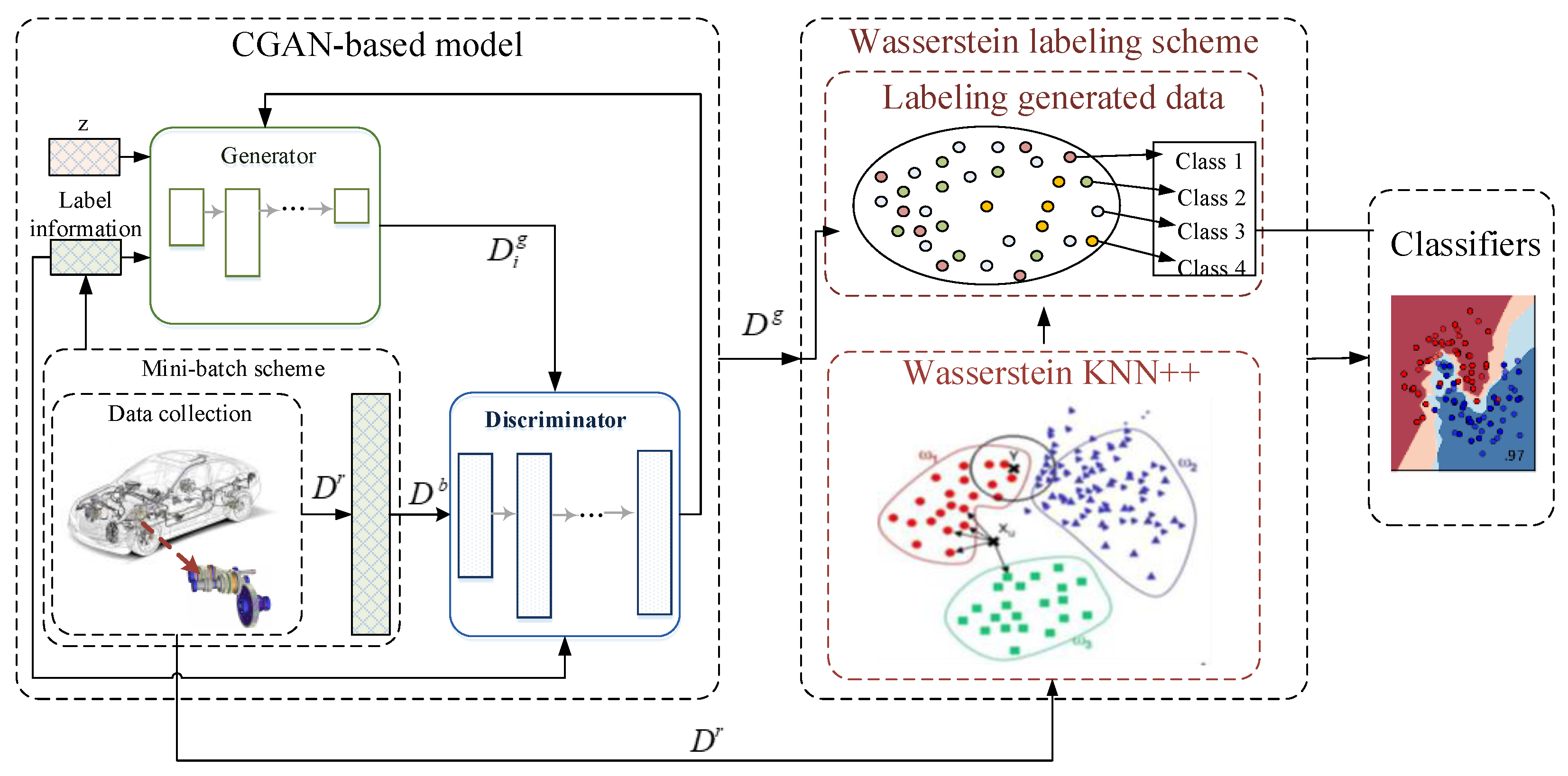
To address reliability assessment of vehicle transmission gears without mechanic modeling and particular conditions, the proposed approach contains two components to prepare for the evaluation of gear reliability with existing gear data (illustrated as in Figure 2).

First, we need to process the gear data collected from the factory. When this kind of highly dimensional and small amount of data are directly put into the generator for generation, it will often cause non-convergence of the generation model. Therefore, this step is indispensable. In this step, our input is the original dataset with the same feature dimensions but different amounts of data under different categories. After data processing, the amount of data in different categories will remain balanced to reduce the imbalance between the data. It is convenient for the generation model.

Afterwords, we input low-dimensional noise with label information into the generator of our CGAN-based model. After the convolutional layer mapping, we get the generated data with the same dimension as the original dataset, then put them together into the discriminator. With the help of back propagation, the weight of the convolutional layers will be updated. In order to raise the diversity of generated representations in accordance with the characteristics of the gear data for the vehicle transmission, the mini-batch scheme is designed to sample certain amounts of original data and produced representations instead of training the discrimination with all representations. When the training is completed, our CGAN-based model will generate data with label information. We take out the generated data and remove the labels.

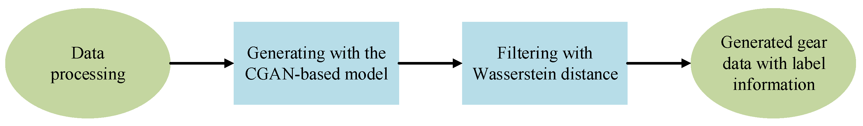
Finally, we input the generated data without label information into the k-nearest neighbor (KNN) model for classification based on Wasserstein distance. Through this model, we can make reasonable annotations for generated data, regardless of whether they coincide in different categories. The flow-process diagram of our proposed method is shown in Figure 3. In addition, the definition of symbols in our article is scattered. We have listed those central and confusing symbols in

Table 1. Symbols used in this section and their interpretation.

Symbol	Description
$P_i$	samples in the real dataset
$Q_i$	feature dimensions of samples in the real dataset
$S_c$	class of samples in the real dataset
$X_i$	$P_i$ after data processing
$A_j$	feature dimensions of $X_i$
$l_c$	class information of $X_i$
$z_i$	noise information into the generator
$D^r$	classification result of the discriminator on $P_i$
$D^g$	discriminator’s classification result of the generated data
$\varpi$	frequency of samples
$J^{\mathcal{D}}$	loss function of the discriminator
$L_t^1$	learning rate of the discriminator
$J^{\mathcal{D}}$	loss function of the discriminator

.

3.1. CGAN-Based Model

3.1.1. Data Processing

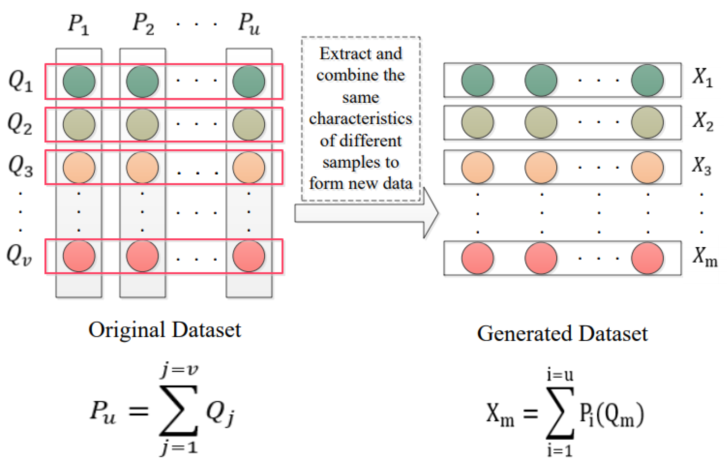
Compared with image data, structured data are close to orthogonal between the various features contained in the data; therefore, for the CGAN-based model, the discriminator cannot pass the gradient back to the generator according to the result of the generator for the iterative update in the processor. Before data generation, we extract and integrate the same features of all data to form a new dataset, as shown in Figure 4, and after our model generates new features, we will merge these features to form new data again; as a result, we obtain an original dataset, with its objects $\left\{P_i\right|i=1,2,\dots ,u\}$, its number of instances u, with its attribute set $\left\{Q_j\right|j=1,2,\dots ,v\}$, its number of attributes v, with its categories $\left\{S_c\right|c=1,2,\dots ,w\}$ and its number of categories w. For the input of the network, a new dataset is constructed, and use D to represent this dataset, with its objects $\left\{X_i\right|i=1,2,\dots ,m\}$, its number of instances m equal to v, with its attribute set $\left\{A_j\right|j=1,2,\dots ,d\}$, its number of attributes d equal to u, with its categories $\left\{l_c\right|c=1,2,\dots ,l\}$ and its number of categories l equal to v; $D^r(m^r,l,d)$ addresses real gear data and $D^g(m^g,l,d)$ represents produced data from our trained generator.

3.1.2. Model Structure

Due to the discrete nature of gear tooth data, when a single GAN is used to generate gear tooth data, the boundaries between different types of generated data are often blurred according to unconditional constraints, especially when similar to gear wheels. The gear data forms a dataset with a small gap between classes, so our generative model uses CGAN with conditional information.

$\mathcal{G}$ and $\mathcal{D}$ in our CGAN-based model are both a neural network with multiple hidden layers. The minimax game is denoted as:   

$$\begin{array}{cc}\hfill \underset{\mathcal{G}}{min}\underset{\mathcal{D}}{max}v(\mathcal{D},\mathcal{G})& =E_{x\sim p_r\left(x\right)}\left[log\mathcal{D}(x,l)\right]\hfill \\ \hfill & +E_{z\sim p_z\left(z\right)}[log(1-\mathcal{D}\left(\mathcal{G}(z,l)\right)]\hfill \end{array}$$

(2)

Mathematically, the solution of this game is to learn the joint probability function other than the probability function in GAN.

In terms of $\mathcal{G}$, noise variables z and label information l are inputs and forged data $D_t^g$ are outputs. t is the iteration time. In the process of generating CGAN, the noise is used as an input for the purpose of making the network random, which can generate very complex distributions. The goal is to make it close to the distribution generated by real data. For the gear data we used, although we have combined these discrete data into a continuous distribution, the randomly added noise will not purposefully make our data distribution more in line with the real data distribution. When the dimension of the input noise is smaller than the amount of data contained in a single gear dataset, this noise will make our data more confusing. Therefore, in the process of CGAN generation, we placed a restriction on the noise according to the characteristics of the data, that is, the dimension of the noise must not be lower than the amount of data contained in a single gear dataset. For $\mathcal{D}$, gear samples x from $D^r$ and $D^g$ are inputs, and the computation result of objective function (Equation (3)) is an output.

$$\begin{array}{cc}\hfill J^{\mathcal{D}}=& -{\displaystyle \frac{1}{2m}}(\sum _{i=1}^{m}log\mathcal{D}(x_i,l_i)+\sum _{i=1}^{m}log(1-\mathcal{D}(\mathcal{G}(z_i,l_i),l_i))\hfill \\ \hfill & s.t.Dimension\left(z\right)>v\hfill \end{array}$$

(3)

The details of our CGAN-based model are in Algorithm 1.

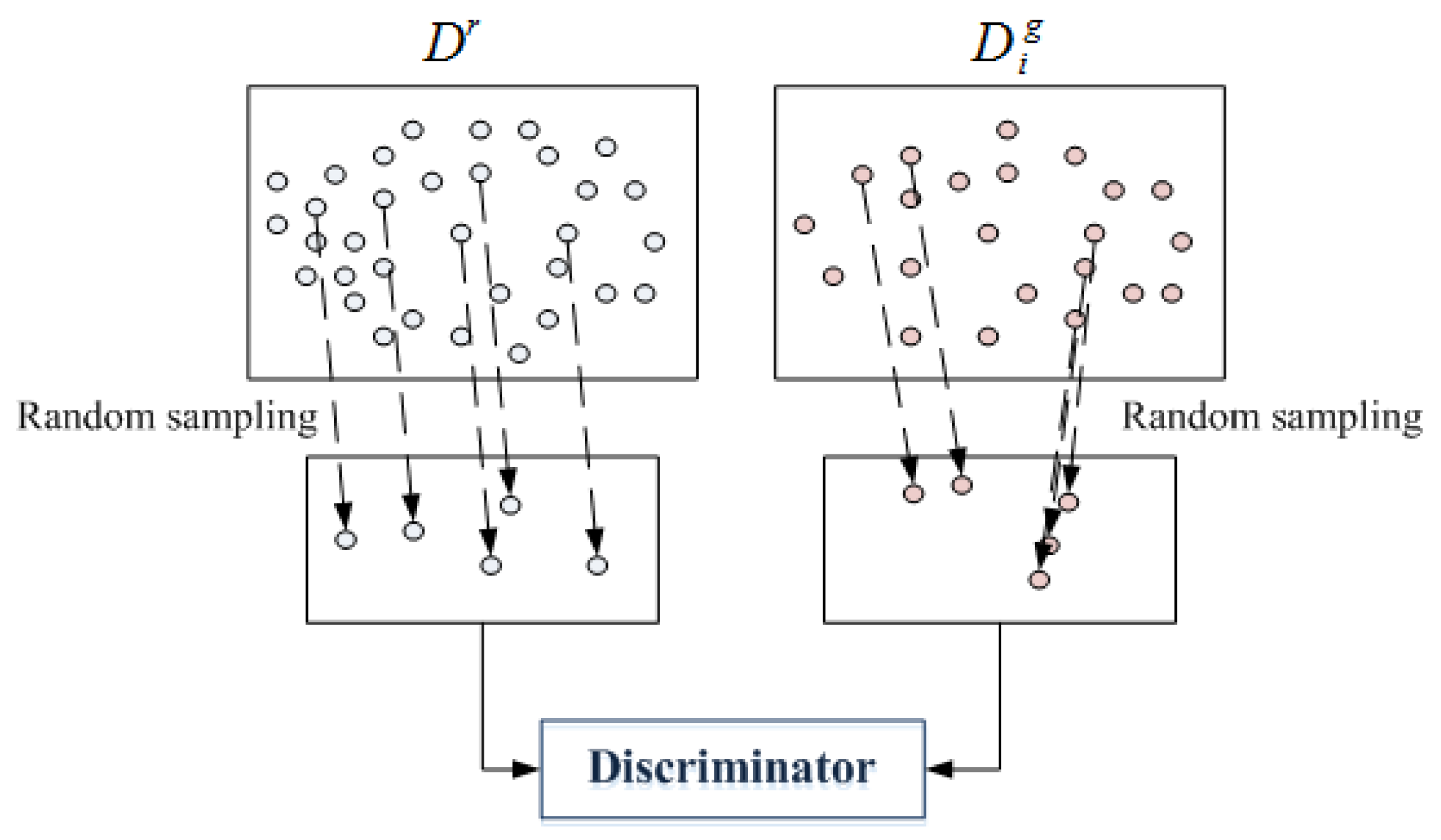
3.1.3. Mini-Batch Scheme

Typically, $\mathcal{G}$ would collapse due to the parameter settings, leading to the production of representations in one model. Thereby, to guarantee the diversity of generated representations, we adopt the mini-batch strategy on $\mathcal{D}$ as shown in Figure 5.

Suppose that b is the mini-batch size, we stochastically sample b representations from $D^r$ as $D^b(m^b,l,d)$ and $D^g$. Instead of accessing the entire $D^r$ and $D^g$, we load $D^b$ into $\mathcal{D}$ to compare with part of generated representations $D^g$.

$$D^b=\left\{x_i\right|x_1,x_2,\dots ,x_b;x_i\in D^r\},m^b<m^r$$

(4)

where $m^b$ and $m^r$ are the number of representations in $D^b$ and $D^r$.

The advantage of this strategy is that $D^g$ is confronted with different real representations in every iteration. The generated representations at each iteration is compared with a portion of real representations, which enhances the diversity of generated representations.    

Algorithm 1: CGAN-based model for extracting the generated representations without label information

3.1.4. Network Optimization

Due to the high density and small amount of gear data, the generated representations are easily trapped into a group of a similar sample to the original. Although the mini-batch scheme is designed to deal with the overfitting issue, one category of gear data has an extremely small size, which aggravates the non-convergence problem. Therefore, instead of gradient descent method for ${\nabla }_{\Phi \left(\mathcal{G}\right)}$ and ${\nabla }_{\Phi \left(\mathcal{D}\right)}$ in GAN, we implement the Adamax optimizer to train both $\mathcal{G}$ and $\mathcal{D}$, which computes exponential moving averages of gradients $\{{\nabla }_{\Phi \left(\mathcal{G}\right)},{\nabla }_{\Phi \left(\mathcal{D}\right)}\}$ and Hessian matrices $\{H_{\Phi \left(\mathcal{G}\right)},H_{\Phi \left(\mathcal{D}\right)}\}$ and provides a simpler range for the upper limit of the learning rate. Exponential decay rates are controlled by coefficients $\{{\eta }_{11},{\eta }_{12},{\eta }_{21},{\eta }_{22}\}\in [0,1)$, which are updated at each iteration. $L_t^1$ and $L_t^2$ represent the learning rates of the gradient with first order, and Hessian matrices are defined as:

$$|L_t^1|\le L_d$$

(5)

$$|L_t^2|\le L_g$$

(6)

where $L_g$ and $L_d$ are initial learning rates of $\mathcal{G}$ and $\mathcal{D}$, respectively. The estimations of the first moment gradient and Hessian matrices at iteration t are given as:   

$$\left\{\begin{array}{c}E{\left({\nabla }_{\Phi \left(\mathcal{D}\right)}\right)}_t={\eta }_{11}·E{\left({\nabla }_{\Phi \left(\mathcal{D}\right)}\right)}_{t-1}+(1-{\eta }_{11})·{\varrho }_t^{\mathcal{D}}\hfill \\ E{\left({\nabla }_{\Phi \left(\mathcal{G}\right)}\right)}_t={\eta }_{21}·E{\left({\nabla }_{\Phi \left(\mathcal{G}\right)}\right)}_{t-1}+(1-{\eta }_{21})·{\varrho }_t^{\mathcal{G}}\hfill \\ E{\left(H_{\Phi \left(\mathcal{D}\right)}\right)}_t=max({\eta }_{12}·E{\left(H_{\Phi \left(\mathcal{D}\right)}\right)}_{t-1},|{\varrho }_t^{\mathcal{D}}\left|\right)\hfill \\ E{\left(H_{\Phi \left(\mathcal{G}\right)}\right)}_t=max({\eta }_{22}·E{\left(H_{\Phi \left(\mathcal{G}\right)}\right)}_{t-1},|{\varrho }_t^{\mathcal{G}}\left|\right)\hfill \end{array}\right.$$

(7)

where ${\varrho }_t^{\mathcal{D}}$ and ${\varrho }_t^{\mathcal{G}}$ are gradients, computed with the following formulas:

$$\left\{\begin{array}{c}{\varrho }_t^{\mathcal{G}}={\nabla }_{\Phi \left(\mathcal{G}\right)}{f}_t(\Phi {\left(\mathcal{G}\right)}_{t-1})\hfill \\ {\varrho }_t^{\mathcal{D}}={\nabla }_{\Phi \left(\mathcal{D}\right)}{f}_t(\Phi {\left(\mathcal{D}\right)}_{t-1})\hfill \end{array}\right.$$

(8)

$\Phi \left(\mathcal{D}\right)$ and $\Phi \left(\mathcal{G}\right)$ are updated as follows.

$$\left\{\begin{array}{c}\Phi {\left(\mathcal{D}\right)}_t=\Phi {\left(\mathcal{D}\right)}_{t-1}-({\displaystyle \frac{L(\Phi (\mathcal{D}\left)\right)}{1-{\eta }_{11}^t}})·{\displaystyle \frac{E{\left({\nabla }_{\Phi \left(\mathcal{D}\right)}\right)}_t}{E{\left(H_{\Phi \left(\mathcal{D}\right)}\right)}_t}}\hfill \\ \Phi {\left(\mathcal{G}\right)}_t=\Phi {\left(\mathcal{G}\right)}_{t-1}-({\displaystyle \frac{L(\Phi (\mathcal{G}\left)\right)}{1-{\eta }_{21}^t}})·{\displaystyle \frac{E{\left({\nabla }_{\Phi \left(\mathcal{G}\right)}\right)}_t}{E{\left(H_{\Phi \left(\mathcal{G}\right)}\right)}_t}}\hfill \end{array}\right.$$

(9)

The ${\eta }_{11},{\eta }_{12},{\eta }_{21},{\eta }_{22}$ and $\epsilon$ are hyperparameters initialized with empirical evidence in the simulation. In the training process of the network, the reason why we use Adamax instead of the Adam that comes with CGAN is because Adam’s ability to adjust the learning rate changes based on a simpler range for the upper limit of the learning rate, as shown in (9). The definition of this range allows our network to process discrete data without modifying the initialization deviation, and has a more flexible adjustment method and a smaller magnitude of change.

3.2. Wasserstein Labeling Scheme

Considering that $D^g$ from our CGAN-based model has no labels, it is necessary to tag the generated representations for classification. With regards to one specific property of gear data [22], general distance measurement (e.g., Euclidean and cosine distance) cannot display well on transmission gear data. To label generated gear representations, the Wasserstein labeling scheme is proposed with a three-step process. First, a Wasserstein barycenter for gear data in each category of gear reliability is discovered by the k-nearest neighbor Wasserstein clustering algorithm. Then, the Wasserstein distance between each sample in the generated data and each Wasserstein barycenter is estimated by the Wasserstein critic. The details are shown in Algorithm 2.

3.2.1. Wasserstein Barycenter

We use $\Pi (D^r,D^g)$ to represent all possible joint distribution combinations of $D^r$ and $D^g$ distribution combinations for each joint distribution $\gamma$ that can be sampled, and the distance between the samples can be calculated. Under the joint distribution $\gamma$, the expected value $E_{(x,y)\sim \gamma }\left[\right||x-y\left|\right|]$ of the sample to the distance is obtained. At this time, we can define the earth-mover (EM) distance between the two samples as the lower bound of the expected value, as shown in the following formula.

$$EM(x,y)=in{f}_{\gamma \sim \pi (D^r,D^g)E_{(x,y)\sim \gamma }\left[\right||x-y\left|\right|]}$$

(10)

Algorithm 2: Wasserstein labeling scheme for assigning labels to the generated representations

The solution of finding the Wasserstein barycenter is transformed into optimizing the following formula:

$$arg\underset{W_B}{min}{\displaystyle \frac{1}{m}}\sum _{i=1}^m{W}_p{(W_B,p_r)}^p$$

(11)

where p is the order of the Wasserstein distance, and is initialized as $p=1$. Thus, $W_p$ is termed as W in this paper. Let $\Omega$ be the transmission matrix in EM distance and $Dist$ be the distance matrix,

$$Dist={\left[EM{(x_i,x_j)}^p\right]}_{ij}$$

(12)

Integrate Equation (12) into Equation (11), the optimal problem is changed into:

$$arg\underset{W_B}{min}\sum _{i=1}^{m}tr\left(Dist(W_B,p_r){\Omega }_i^T\right)$$

(13)

Suppose $f(x,\varpi )$ as discrete description of a distribution, x is the value of samples and $\varpi$ is the frequency of samples. Real gear data in each reliability are denoted as $\{D_1^r,D_2^r,D_3^r,D_4^r\}$, respectively. To resolve Equation (13), the Sinkhorn iteration is designed to obtain $\Omega$ of $D_k^r$:

$${\Omega }_i=Sinkhorn({\varpi }_i,{\varpi }_{D_k^r})$$

(14)

Then, the location of the Wasserstein barycenter in $D_k^r$ is solved as:

$$x_k^{WB}={\displaystyle \frac{1}{n}}(\sum _{i=1}^{m_k^r}{x}_i{\left({\Omega }_i\right)}^T)diag({\displaystyle \frac{1}{{\varpi }_i}})$$

(15)

Accordingly, a set of Wasserstein barycenters for gear reliability evaluation with existing gear data is obtained as $\left\{x_k^{WB}\right|k=\{1,2,3,4\}\}$.

3.2.2. Labeling Generated Data

Wasserstein distance between two datasets, take $D^r$ and $D^g$ for example, is given by

$$\begin{array}{cc}\hfill \widehat{W}(p_r,p_g)=& trace\left(Dist{(diag\left(v\right)·\varrho ·diag\left(u\right))}^T\right)\hfill \\ \hfill & s.t.u={\displaystyle \frac{b}{{\varrho }^{T}v}}andv={\displaystyle \frac{a}{\varrho u}}\hfill \end{array}$$

(16)

where $\varrho$ = $exp(-\beta ·Dist(x_i,x_j))$, $x_i\in D^r$ and $x_j\in D^g$; v is a $1\ast n_r$ matrix with all values of 1.

Suppose $x_i$ as ith sample in $D^g$, the Wasserstein distance between x and Wasserstein barycenter $x_k^{WB}$ of kth reliability of transmission gear is denoted as:

$$\begin{array}{cc}\hfill \widehat{W}(x_i,x_k^{WB})=& trace\left(Dist{(diag\left(x_i^T{x}_i\right)·\varrho ·diag\left({\left(x_k^{WB}\right)}^T{x}_k^{WB}\right))}^T\right)\hfill \\ \hfill & s.t.u={\displaystyle \frac{b}{{\varrho }^{T}v}}andv={\displaystyle \frac{a}{\varrho u}}\hfill \\ \hfill & s.t.k=\{1,2,3,4\}\hfill \end{array}$$

(17)

After estimating the distance from each generated sample and each Wasserstein barycenter, the reliability with the minimum distance is used to tag the generated sample.

$$l^{\ast }=arg\underset{k}{min}\widehat{W}(x_i,x_k^{WB})$$

(18)

where $l^{\ast }$ is the label of the generated sample $x_i$.

3.3. Discussion

3.3.1. The Necessity of Data Processing

When analyzing unbalanced data, we use a set of gear data for specific analysis. In this dataset, occurrences of each reliability is 40/44/97/31 from class 1 to 4 and the dimension of each sample is 85. It can be seen that high reliability having the maximum samples is the most common operating condition. Although the number of samples between different categories is quite different, we can find that all samples have the same dimensional characteristics. The difference between gear data and other data is that the same dimensions represent the same characteristics. Therefore, we reorganize data in the same category according to feature dimensions. We also select them through the mini-batch scheme and form four categories with the same number of samples. For example, the samples in the first category are 85 and each has 40 dimensional features. Samples in the second class are also 85 and each has 40 dimensional features. We will discard the extra samples and repeat part of the data. In this method, CGAN improves performance in generating different classes of samples.

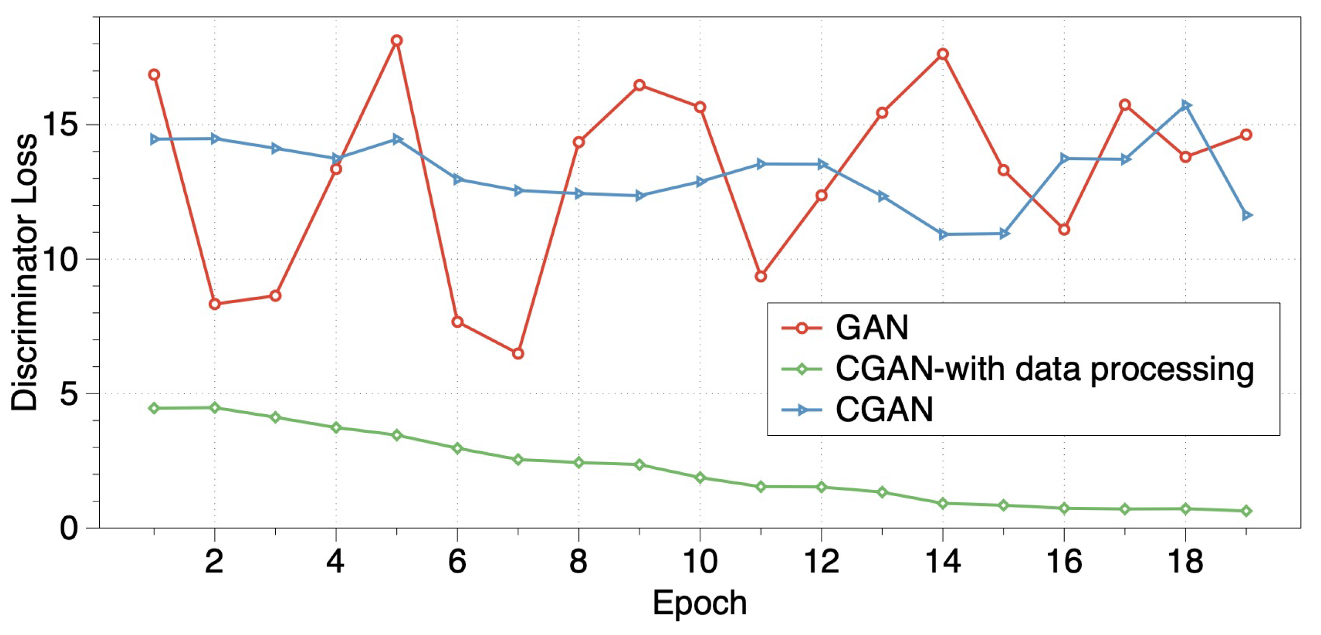
In order to analyze the performance of data processing, we observe the values of loss functions by using both our CGAN-based model and traditional GAN for transmission gear data. The results are shown in Figure 6. When data processing is not used in the training process, loss values fluctuate with training epochs, which means that GAN and CGAN are unable to learn the right mapping relationship directly from the transmission gear data. After data processing is used in CGAN, the loss values are steadily declining with training epochs, which shows that the imbalance class issues are lightened.

3.3.2. Algorithm Performance

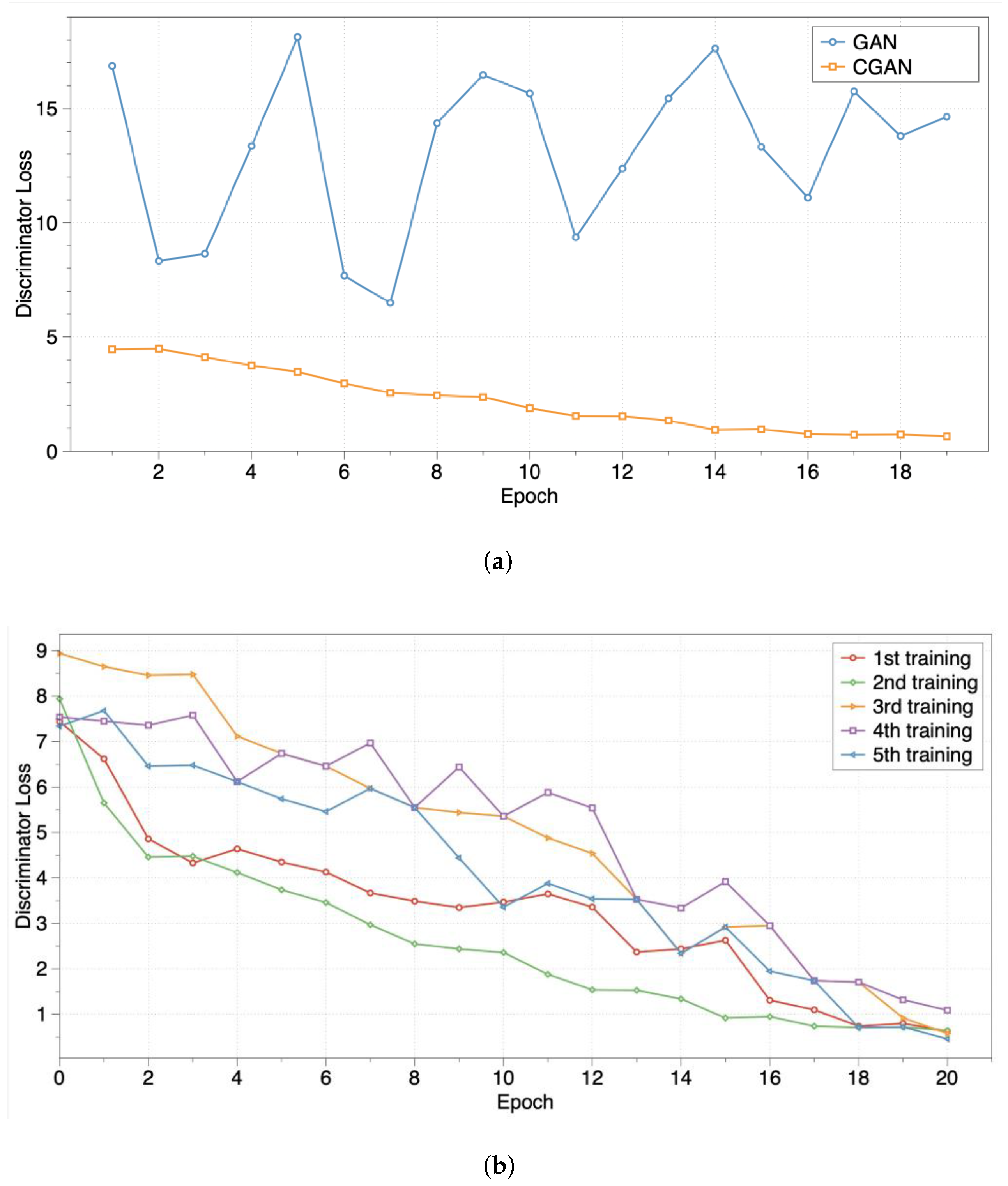
The method consists of Algorithms 1 and 2. In the CGAN-based model in Algorithm 1, we can generate new samples without label information in different class spaces. Then, generated data are filtered according to the Wasserstein distance in Algorithm. In order to explore the stability and convergence of these two algorithms, we observe the values of loss functions [33] by using both our CGAN-based model and traditional GAN for transmission gear data. From Figure 7a, discriminator loss values in Algorithm 1 are gradually decreasing with a consistent trend, whereas those values of the traditional GAN have uncertain fluctuations. This indicates that the convergence of our CGAN-based model is more stable on gear data than the traditional GAN. Furthermore, to avoid training randomness, we trained our CGAN-based model five times. Loss function curves of discriminator loss (as illustrated in Figure 7b) have parallel trends. The loss values are decreasing with training epochs, which shows that our model has effective stability and required convergence for transmission gear data.

4. Results

4.1. Simulation Settings

Experimental gear data are provided by a transmission company named Qingshan industry, and is a real-world gear dataset including 212 items. In the dataset, the occurrences of each reliability is $40/44/97/31$ from class 1 to 4 and the dimension of each sample is 85. It can be seen that high reliability having the maximum samples is the most common operating conditions.

The CGAN-based model in our approach was simulated on a single NVIDIA TITAN Xp GPU. All simulations ran on an Intel i7-6800K CPU. The output layer of the generator and the input layer of the discriminator both contain 212 neurons, manipulated by the size of the gear parameters. Other sizes of the generator are $\{128,1024,256\}$ and that of the discriminator are $\{256,1024,128\}$. The input of the CGAN generator is a random noise and its dimension is 212. Through the convolution layers of the generator, random noise was mapped into higher dimensions and judged by discriminator. After noise passes through generator convolutional layers, which are $\{128,1024,256\}$, noise becomes a $256\ast 1$ feature vector. The convolutional layers that are designed as $\{256,1024,128\}$ are used for feature extraction. At the end, it passes through a softMax layer for classification.

Moreover, weight initialization in these two networks follows the distribution $U[-\sqrt{3}/\sqrt{32},\sqrt{3}/\sqrt{32}]$. The learning of parameters in the training process is optimized based on the gradient descent algorithm. This algorithm needs to assign an initial value at the beginning of training. In our experiment, one of the problems was how to choose the way of random initialization. Considering the softMax layer in our network, we decide to use uniform distribution initialization. Hence, there is a good distinction between neurons in different layers [34].

4.2. Model Parameter Analysis

We investigate the effect of a hyperparameter, i.e., mini-batch size $m^b$, described in the mini-batch strategy of our CGAN-based model. For a clear mathematical description, $\zeta =m^b/m^r$ is sampled from $\{60\%,70\%,80\%,90\%,100\%\}$. The number of generated samples in each degree is obtained with different $\zeta$. Simulation results are shown in Figure 8, in which the diversity is preferable when $\zeta =80\%$. While the value of $\zeta$ is small, the training dataset contains less samples in the smallest group of reliability degree (e.g., Degree 4), leading to the inadequate learning of this degree and the generation of infrequent samples in Degree 4. Interestingly, when the value of $\zeta$ increased to $90\%$ and $100\%$, the imbalance among the number of all degrees becomes greater, which suffers from mode collapse in GAN. As such, in this paper, to ensure the diversity of generated data from our approach, $\zeta$ is set to $80\%$.

4.3. Comparisons of Different Labeling Strategy

To validate the effectiveness of proposed WL scheme, we compared the approach with other labeling strategies: a labeling scheme based on cosine and Euclidean distance. Two different classifiers (i.e., decision tree and multilayer perceptron) and four indicators (i.e., precise, recall, F-measure and G-mean) were implemented to evaluate the performance of expanded data. The results are shown in Figure 9, where red lines are averaged results within 10 runs and blue boxes are performance intervals of these 10 runs.

Note that the proposed CGAN-WL plays effectively on gear data in all indicators even while using different classifiers. This discovery provides further verification on the theory that gear parameters have strong coupled relations between each others while general distance measurements (e.g., Euclidean distance) cannot display effectively on gear data.

4.4. Comparisons of Different Generation Methods

To observe the credibility of generated samples from our approach, we compared our approach to six other techniques for expanding gear data. Five compared techniques were sourced from the imbalanced-learn API toolbox [35]: random oversampling (ROS), synthetic minority oversampling technique (SMOTE), adaptive synthetic sampling (ADASYN), synthetic minority oversampling technique-edited nearest neighborhood (SMOTEENN) and synthetic minority oversampling technique-Tomek link (SMOTETomek). Furthermore, we make the contrast of giving labels to produced samples from GAN using WL (GAN-WL). In the simulation, m (representing the number of nearest neighbors that identify if minority samples are on the spot) is set to 15, and k (addressing the number of nearest neighbors that are synthetic samples) is initialized as 10.

Both simple metrics (i.e., recall (R) and precise (P)) and comprehensive metrics (i.e., G-mean (G-M) and F-measure (F-M)) are used to score the results of gear reliability assessment. Higher values of these indicators imply better performance. These metrics are denoted with the given Equation (19), where $FP$ is the amount of negative instances that are misclassified; $TP$ is the amount of positive instances that are classified properly; $FN$ is the amount of positive instances that are misclassified; $TN$ is the amount of negative instances that are classified properly.

$$\begin{array}{cc}\hfill & R={\displaystyle \frac{TP}{TP+FN}}P={\displaystyle \frac{TP}{TP+FP}}\hfill \\ \hfill & G-M=\sqrt{{\displaystyle \frac{TN}{TN+FP}}·R}\hfill \\ \hfill & F-M={\displaystyle \frac{2·R·P}{R+P}}\hfill \end{array}$$

(19)

Considering the specifications of various classifiers, we implement three kinds of classifiers in the scikit-learn toolbox [36] to discover the performance of gear reliability evaluation using different classification techniques: decision tree (DT), random forest (RF) and multilayer perceptron (MLP). Four-fold cross-validation is used where real-world gear data are stochastically segmented into four folds. One fold is used for testing and the remaining three folds are used for training. In order to decrease the influence of sampling randomness in the training–testing process, we ran all classifiers 10 times, and all metric values were averaged over these 10 runs.

Table 2. Averages of metrics by different methods using different classifiers. The bold characters are highlighted as best performances.

Metrics	P	R	F-M	G-M
Algorithm: DT [36]
ROS [35]	0.791${}_{\pm 0.01}$	0.796${}_{\pm 0.01}$	0.790${}_{\pm 0.01}$	0.843${}_{\pm 0.01}$
SMOTE [21]	0.769${}_{\pm 0.03}$	0.762${}_{\pm 0.03}$	0.762${}_{\pm 0.03}$	0.813${}_{\pm 0.02}$
ADASYN [39]	0.792${}_{\pm 0.03}$	0.796${}_{\pm 0.03}$	0.790${}_{\pm 0.03}$	0.842${}_{\pm 0.02}$
SMOTETomek [35]	0.767${}_{\pm 0.03}$	0.777${}_{\pm 0.03}$	0.763${}_{\pm 0.03}$	0.816${}_{\pm 0.02}$
SMOTEENN [35]	0.674${}_{\pm 0.06}$	0.654${}_{\pm 0.05}$	0.637${}_{\pm 0.04}$	0.746${}_{\pm 0.05}$
GAN-WL	0.802${}_{\pm 0.01}$	0.804${}_{\pm 0.01}$	0.799${}_{\pm 0.01}$	0.832${}_{\pm 0.01}$
CGAN-WL(ours)	0.854${}_{\pm 0.03}$	0.858${}_{\pm 0.3}$	0.852${}_{\pm 0.02}$	0.889${}_{\pm 0.02}$
Algorithm: RF [40]
ROS	0.759${}_{\pm 0.07}$	0.754${}_{\pm 0.01}$	0.749${}_{\pm 0.06}$	0.806${}_{\pm 0.05}$
SMOTE	0.774${}_{\pm 0.05}$	0.769${}_{\pm 0.06}$	0.767${}_{\pm 0.06}$	0.819${}_{\pm 0.04}$
ADASYN	0.788${}_{\pm 0.03}$	0.781${}_{\pm 0.03}$	0.777${}_{\pm 0.03}$	0.828${}_{\pm 0.03}$
SMOTETomek	0.766${}_{\pm 0.03}$	0.758${}_{\pm 0.03}$	0.754${}_{\pm 0.04}$	0.814${}_{\pm 0.02}$
SMOTEENN	0.682${}_{\pm 0.09}$	0.615${}_{\pm 0.09}$	0.613${}_{\pm 0.11}$	0.721${}_{\pm 0.07}$
GAN-WL	0.744${}_{\pm 0.07}$	0.740${}_{\pm 0.07}$	0.735${}_{\pm 0.05}$	0.800${}_{\pm 0.03}$
CGAN-WL(ours)	0.815${}_{\pm 0.01}$	0.815${}_{\pm 0.01}$	0.810${}_{\pm 0.01}$	0.848${}_{\pm 0.01}$
Algorithm: MLP [36]
ROS	0.701${}_{\pm 0.04}$	0.683${}_{\pm 0.05}$	0.678${}_{\pm 0.05}$	0.751${}_{\pm 0.03}$
SMOTE	0.686${}_{\pm 0.05}$	0.671${}_{\pm 0.06}$	0.670${}_{\pm 0.06}$	0.741${}_{\pm 0.04}$
ADASYN	0.709${}_{\pm 0.04}$	0.696${}_{\pm 0.04}$	0.694${}_{\pm 0.04}$	0.760${}_{\pm 0.03}$
SMOTETomek	0.698${}_{\pm 0.03}$	0.675${}_{\pm 0.04}$	0.677${}_{\pm 0.03}$	0.758${}_{\pm 0.02}$
SMOTEENN	0.625${}_{\pm 0.06}$	0.539${}_{\pm 0.06}$	0.503${}_{\pm 0.05}$	0.652${}_{\pm 0.08}$
GAN-WL	0.593${}_{\pm 0.04}$	0.596${}_{\pm 0.04}$	0.589${}_{\pm 0.04}$	0.688${}_{\pm 0.04}$
CGAN-WL(ours)	0.756${}_{\pm 0.02}$	0.762${}_{\pm 0.03}$	0.749${}_{\pm 0.02}$	0.798${}_{\pm 0.02}$

examines the performance of classification with various generative techniques. Clearly, the proposed CGAN-WL outperforms other compared techniques both using the three classifiers. It can be seen that other compared techniques display unstably with different classifiers. Take GAN-WL for example, it operates well with DT but works bad with MLP. SMOTE and its variations (i.e., ADASYN, SMOTETomek and SMOTEENN) based on Euclidean distance measurement are not capable to discovery the relation between gear data and its reliability. To further prove the enhancement in statistical ways, we implement both Welch’s T-test [37] and Mann–Whitney U test [38] to assess the significance of the improvement. Comparisons between the proposed approach and compared techniques are observed with three classifiers. With a significance level at 0.05, test results of all metrics are illustrated in

Table 3. Summary of Welch’s T-test with significance level at 0.05 using three classifiers.

	Method	DT [36]	RF [40]	MLP [36]
P	ROS [35]	$5.353\times {10}^{-5}$	$4.437\times {10}^{-4}$	$6.674\times {10}^{-7}$
	SMOTE [21]	$2.067\times {10}^{-5}$	$2.680\times {10}^{-3}$	$2.917\times {10}^{-8}$
	ADASYN [39]	$3.466\times {10}^{-4}$	$3.629\times {10}^{-4}$	$3.739\times {10}^{-6}$
	SMOTETomek [35]	$6.601\times {10}^{-5}$	$7.669\times {10}^{-5}$	$2.118\times {10}^{-13}$
	SMOTEENN [35]	$1.084\times {10}^{-5}$	$2.424\times {10}^{-9}$	$4.430\times {10}^{-15}$
	CGAN-WL(ours)	$1.766\times {10}^{-5}$	$8.123\times {10}^{-7}$	$8.883\times {10}^{-7}$
R	ROS	$2.382\times {10}^{-5}$	$1.700\times {10}^{-3}$	$5.925\times {10}^{-7}$
	SMOTE	$3.188\times {10}^{-4}$	$1.531\times {10}^{-4}$	$5.015\times {10}^{-7}$
	ADASYN	$1.106\times {10}^{-4}$	$1.600\times {10}^{-3}$	$4.597\times {10}^{-7}$
	SMOTETomek	$4.265\times {10}^{-5}$	$3.049\times {10}^{-5}$	$2.775\times {10}^{-14}$
	SMOTEENN	$3.345\times {10}^{-7}$	$3.403\times {10}^{-13}$	$8.132\times {10}^{-20}$
	CGAN-WL(ours)	$2.637\times {10}^{-5}$	$1.812\times {10}^{-5}$	$1.384\times {10}^{-8}$
F-M	ROS	$3.656\times {10}^{-4}$	$2.200\times {10}^{-3}$	$1.581\times {10}^{-5}$
	SMOTE	$3.556\times {10}^{-5}$	$3.730\times {10}^{-4}$	$6.694\times {10}^{-7}$
	ADASYN	$2.244\times {10}^{-5}$	$9.400\times {10}^{-3}$	$3.845\times {10}^{-7}$
	SMOTETomek	$3.970\times {10}^{-5}$	$1.863\times {10}^{-5}$	$7.607\times {10}^{-14}$
	SMOTEENN	$9.065\times {10}^{-7}$	$1.778\times {10}^{-12}$	$4.114\times {10}^{-20}$
	CGAN-WL(ours)	$6.657\times {10}^{-6}$	$9.514\times {10}^{-7}$	$9.085\times {10}^{-8}$
G-M	ROS	$2.795\times {10}^{-5}$	$3.609\times {10}^{-4}$	$4.798\times {10}^{-8}$
	SMOTE	$2.507\times {10}^{-5}$	$4.300\times {10}^{-3}$	$2.273\times {10}^{-7}$
	ADASYN	$9.941\times {10}^{-4}$	$3.000\times {10}^{-3}$	$1.192\times {10}^{-5}$
	SMOTETomek	$1.495\times {10}^{-5}$	$1.408\times {10}^{-4}$	$2.705\times {10}^{-12}$
	SMOTEENN	$1.147\times {10}^{-6}$	$3.376\times {10}^{-11}$	$4.279\times {10}^{-17}$
	CGAN-WL(ours)	$6.771\times {10}^{-6}$	$2.335\times {10}^{-6}$	$5.426\times {10}^{-6}$

. The values of all metrics are all lower than 0.5, which indicates the proposed approach observably outperforms the compared methods.

In order to verify the effectiveness of our method more effectively, we ran our test on a standard dataset from UCI (called refractive errors dataset (RED)) [41]. The aim of this dataset is to study the impact of personal lifestyle and genetics on eye refractive errors. This dataset is gathered from forms filled out by 467 individuals. The first sheet contains the information of 210 people suffering from eye refractive errors and the second sheet contains information of the remaining 257 participants, which had a healthy eye condition. This discrete data are similar to our gear dataset, and the test results are shown in

Table 4. Averages of metrics by different methods using different classifiers on the Refractive errors DataSet [41]. The bold characters are highlighted as the best performances.

Metrics	P	R	F-M	G-M
Algorithm: DT [36]
ROS [35]	0.753${}_{\pm 0.03}$	0.757${}_{\pm 0.02}$	0.751${}_{\pm 0.01}$	0.802${}_{\pm 0.01}$
SMOTE [21]	0.725${}_{\pm 0.02}$	0.727${}_{\pm 0.02}$	0.729${}_{\pm 0.01}$	0.776${}_{\pm 0.03}$
ADASYN [39]	0.758${}_{\pm 0.05}$	0.754${}_{\pm 0.01}$	0.756${}_{\pm 0.03}$	0.801${}_{\pm 0.02}$
SMOTETomek [35]	0.725${}_{\pm 0.02}$	0.727${}_{\pm 0.04}$	0.720${}_{\pm 0.04}$	0.771${}_{\pm 0.01}$
SMOTEENN [35]	0.638${}_{\pm 0.05}$	0.616${}_{\pm 0.04}$	0.599${}_{\pm 0.03}$	0.704${}_{\pm 0.06}$
GAN-WL	0.766${}_{\pm 0.02}$	0.760${}_{\pm 0.02}$	0.759${}_{\pm 0.01}$	0.801${}_{\pm 0.02}$
CGAN-WL(ours)	0.811${}_{\pm 0.02}$	0.817${}_{\pm 0.1}$	0.817${}_{\pm 0.03}$	0.846${}_{\pm 0.02}$
Algorithm: RF [40]
ROS	0.715${}_{\pm 0.07}$	0.717${}_{\pm 0.01}$	0.706${}_{\pm 0.06}$	0.766${}_{\pm 0.05}$
SMOTE	0.737${}_{\pm 0.05}$	0.725${}_{\pm 0.06}$	0.728${}_{\pm 0.06}$	0.775${}_{\pm 0.04}$
ADASYN	0.746${}_{\pm 0.03}$	0.745${}_{\pm 0.03}$	0.737${}_{\pm 0.03}$	0.781${}_{\pm 0.03}$
SMOTETomek	0.723${}_{\pm 0.03}$	0.719${}_{\pm 0.03}$	0.711${}_{\pm 0.04}$	0.776${}_{\pm 0.02}$
SMOTEENN	0.642${}_{\pm 0.09}$	0.585${}_{\pm 0.09}$	0.583${}_{\pm 0.11}$	0.687${}_{\pm 0.07}$
GAN-WL	0.703${}_{\pm 0.07}$	0.701${}_{\pm 0.07}$	0.705${}_{\pm 0.05}$	0.760${}_{\pm 0.03}$
CGAN-WL(ours)	0.776${}_{\pm 0.01}$	0.775${}_{\pm 0.01}$	0.779${}_{\pm 0.01}$	0.808${}_{\pm 0.01}$
Algorithm: MLP [36]
ROS	0.681${}_{\pm 0.02}$	0.679${}_{\pm 0.04}$	0.679${}_{\pm 0.04}$	0.711${}_{\pm 0.03}$
SMOTE	0.641${}_{\pm 0.04}$	0.636${}_{\pm 0.05}$	0.631${}_{\pm 0.03}$	0.702${}_{\pm 0.02}$
ADASYN	0.667${}_{\pm 0.03}$	0.656${}_{\pm 0.03}$	0.654${}_{\pm 0.04}$	0.727${}_{\pm 0.02}$
SMOTETomek	0.651${}_{\pm 0.02}$	0.637${}_{\pm 0.05}$	0.646${}_{\pm 0.03}$	0.719${}_{\pm 0.04}$
SMOTEENN	0.585${}_{\pm 0.05}$	0.508${}_{\pm 0.05}$	0.501${}_{\pm 0.01}$	0.617${}_{\pm 0.04}$
GAN-WL	0.556${}_{\pm 0.03}$	0.557${}_{\pm 0.04}$	0.541${}_{\pm 0.05}$	0.640${}_{\pm 0.03}$
CGAN-WL(ours)	0.716${}_{\pm 0.04}$	0.728${}_{\pm 0.02}$	0.703${}_{\pm 0.02}$	0.778${}_{\pm 0.03}$

. We can see that other compared techniques are unstable with different classifiers. It can be found that compared to other methods, CGAN-WL can learn better conditional mapping from discrete dataset, and use WL to make reasonable annotations.

5. Conclusions

Gear reliability evaluation was found to be remarkable at guaranteeing the safety of vehicle operations. This paper proposed a CGAN-WL approach to deal with gear reliability assessment when collected gear data were insufficient. To find the prior value of hyperparameter b in the approach, the diversity of generated representations with different b was observed. Furthermore, in order to demonstrate the effectiveness of our approach, different labeling schemes were conducted to work on gear data. Simulation results revealed the effectiveness of our approach and validated the characteristics of gear data that show that the relations among gear parameters were tight. Finally, with three different classifiers in the experiments, CGAN-WL outperformed other popular generative techniques in both simple and complicated metrics. Statistical tests further proved the significant improvement of our approach. In the future, we intend to work on the transmission gear data of electric vehicles. The transmission of an electric vehicle adopts a fixed rate in gear data. Gear clearance tends to larger, and noise generated by the transmission is weakened. So the overlap in different classes of gear data becomes smaller, which brings great challenges to traditional identification methods.

References

1. Dong, L.; Li, Z.; Zhou, Q.; Zhang, Z. Research on Reliability Test Method of Product Formulation. Reliab. Environ. Test. Electron. Prod. 2021, 39, 7–11. [Google Scholar]
2. Li, J.; He, H.; Li, L.; Chen, G. A Novel Generative Model with Bounded-GAN for Reliability Classification of Gear Safety. IEEE Trans. Ind. Electron. 2019, 66, 8772–8781. [Google Scholar] [CrossRef]
3. Wang, Z.; Gao, J.M.; Wang, R.X.; Chen, K.; Gao, Z.Y.; Zheng, W. Failure mode and effects analysis by using the house of reliability-based rough VIKOR approach. IEEE Trans. Reliab. 2018, 67, 230–248. [Google Scholar] [CrossRef]
4. Park, J.; Ha, J.M.; Oh, H.; Youn, B.D.; Choi, J.H.; Kim, N.H. Model-based fault diagnosis of a planetary gear: A novel approach using transmission error. IEEE Trans. Reliab. 2016, 65, 1830–1841. [Google Scholar] [CrossRef]
5. Xu, S.; Li, S.E.; Bo, C.; Li, K. Instantaneous Feedback Control for a Fuel-Prioritized Vehicle Cruising System on Highways With a Varying Slope. IEEE Trans. Intell. Transp. Syst. 2017, 18, 1210–1220. [Google Scholar] [CrossRef]
6. Gao, B.; He, Y.; Woo, W.L.; Tian, G.Y.; Liu, J.; Hu, Y. Multidimensional tensor-based inductive thermography with multiple physical fields for offshore wind turbine gear inspection. IEEE Trans. Ind. Electron. 2016, 63, 6305–6315. [Google Scholar] [CrossRef] [Green Version]
7. Tan, X.; Xie, L. Fatigue Reliability Evaluation Method of a Gear Transmission System Under Variable Amplitude Loading. IEEE Trans. Reliab. 2019, 68, 599–608. [Google Scholar] [CrossRef]
8. Zhao, B.; Xie, L.; Li, H.; Zhang, S.; Wang, B.; Li, C. Reliability Analysis of Aero-Engine Compressor Rotor System Considering Cruise Characteristics. IEEE Trans. Reliab. 2019, 69, 245–259. [Google Scholar] [CrossRef]
9. Gabdullin, N.; Madanzadeh, S.; Vilkin, A. Towards End-to-End Deep Learning Performance Analysis of Electric Motors. Actuators 2021, 10, 28. [Google Scholar] [CrossRef]
10. Li, W.W.K. On a mixture autoregressive model. J. R. Stat. Soc. 2010, 62, 95–115. [Google Scholar]
11. Zhu, Y.; Zhou, G. Technical analysis: An asset allocation perspective on the use of moving averages. J. Financ. Econ. 2009, 92, 519–544. [Google Scholar] [CrossRef]
12. Abrahart, R.J.; See, L. Comparing neural network and autoregressive moving average techniques for the provision of continuous river flow forecasts in two contrasting catchments. Hydrol. Process. 2015, 14, 2157–2172. [Google Scholar] [CrossRef]
13. Ouyang, T.; He, Y.; Huang, H. Monitoring Wind Turbines’ Unhealthy Status: A Data-Driven Approach. IEEE Trans. Emerg. Top. Comput. Intell. 2018, 3, 163–172. [Google Scholar] [CrossRef]
14. Jiang, G.; Xie, P.; He, H.; Yan, J. Wind turbine fault detection using a denoising autoencoder with temporal information. IEEE/ASME Trans. Mechatron. 2018, 23, 89–100. [Google Scholar] [CrossRef]
15. Jiang, G.; He, H.; Xie, P.; Tang, Y. Stacked multilevel-denoising autoencoders: A new representation learning approach for wind turbine gearbox fault diagnosis. IEEE Trans. Instrum. Meas. 2017, 66, 2391–2402. [Google Scholar] [CrossRef]
16. Lu, D.; Qiao, W.; Gong, X. Current-based gear fault detection for wind turbine gearboxes. IEEE Trans. Sustain. Energy 2017, 8, 1453–1462. [Google Scholar] [CrossRef]
17. Preechayasomboon, P.; Rombokas, E. Sensuator: A Hybrid Sensor–Actuator Approach to Soft Robotic Proprioception Using Recurrent Neural Networks. Actuators 2021, 10, 30. [Google Scholar] [CrossRef]
18. Lim, P.; Goh, C.K.; Tan, K.C. A Novel Time Series-Histogram of Features (TS-HoF) Method for Prognostic Applications. IEEE Trans. Emerg. Top. Comput. Intell. 2018, 2, 204–213. [Google Scholar] [CrossRef]
19. Xu, W.; Xu, J.X.; He, D.; Tan, K.C. An Evolutionary Constraint-Handling Technique for Parametric Optimization of a Cancer Immunotherapy Model. IEEE Trans. Emerg. Top. Comput. Intell. 2019, 3, 151–162. [Google Scholar] [CrossRef]
20. He, H.; Garcia, E.A. Learning from Imbalanced Data. IEEE Trans. Knowl. Data Eng. 2009, 21, 1263–1284. [Google Scholar]
21. Chawla, N.V.; Bowyer, K.W.; Hall, L.O.; Kegelmeyer, W.P. SMOTE: Synthetic Minority Over-sampling Technique. J. Artif. Intell. Res. 2002, 16, 321–357. [Google Scholar] [CrossRef]
22. Li, J.; Liu, S.; He, H.; Li, L. A Novel Framework for Gear Safety Factor Prediction. IEEE Trans. Ind. Inform. 2018, 15, 1998–2007. [Google Scholar] [CrossRef]
23. Tang, L. Two-stage Robust Unit Commitment Considering Wind Power Uncertainty and Unit Failure and Outage Risk. Smart Power 2021, 49, 47–53. [Google Scholar]
24. Sharghi, A.H.; Karami Mohammadi, R.; Farrokh, M.; Zolfagharysaravi, S. Feed-Forward Controlling of Servo-Hydraulic Actuators Utilizing a Least-Squares Support-Vector Machine. Actuators 2020, 9, 11. [Google Scholar] [CrossRef] [Green Version]
25. Goodfellow, I.; Jean, P.A.; Mirza, M.; Xu, B.; David, W.F.; Ozair, S.; Courville, A.; Bengio, Y. Generative adversarial networks. arXiv 2014, arXiv:1406.2661. [Google Scholar] [CrossRef]
26. Yun, B. A manufacturing quality prediction model based on AdaBoost-LSTM with rough knowledge. Comput. Ind. Eng. 2021, 155, 107227. [Google Scholar]
27. Wu, Y.; Zhang, Z.; Xiao, R.; Jiang, P.; Dong, Z.; Deng, J. Operation State Identification Method for Converter Transformers Based on Vibration Detection Technology and Deep Belief Network Optimization Algorithm. Actuators 2021, 10, 56. [Google Scholar] [CrossRef]
28. Xuan, N.; Ding, H.; Qi, M.; Wang, Y.; Wongd, E.K. URCA-GAN: UpSample Residual Channel-wise Attention Generative Adversarial Network for image-to-image translation. Neurocomputing 2021, 443, 75–84. [Google Scholar]
29. Liu, D.; Huang, X.; Zhan, W.; Ai, L.; Zheng, X.; Cheng, S. View synthesis-based light field image compression using a generative adversarial network. Inf. Sci. 2020, 545, 118–131. [Google Scholar] [CrossRef]
30. Yi, X.; Walia, E.; Babyn, P. Generative adversarial network in medical imaging: A review. Med. Image Anal. 2019, 371, 58–67. [Google Scholar] [CrossRef] [Green Version]
31. Fekri, M.N.; Ghosh, A.M.; Grolinger, K. Generating Energy Data for Machine Learning with Recurrent Generative Adversarial Networks. Energies 2019, 13, 130. [Google Scholar] [CrossRef] [Green Version]
32. Tiantian, H.; Song, H.; Jiang, T.; Li, S. Learning Representations of Inorganic Materials from Generative Adversarial Networks. Symmetry 2020, 12, 1889. [Google Scholar]
33. Yong, W.Z.; Ki, K.D. Experimental Analysis of Equilibrization in Binary Classification for Non-Image Imbalanced Data Using Wasserstein GAN. Int. J. Internet 2018, 11, 37–42. [Google Scholar]
34. Fan, Y.; Liu, C. A Neural Network Weight Initialization Method Based on Transfer Learning. CN Patent CN111126599A, 8 May 2020. [Google Scholar]
35. Lemaitre, G.; Nogueira, F.; Aridas, C.K. Imbalanced-learn: A Python Toolbox to Tackle the Curse of Imbalanced Datasets in Machine Learning. J. Mach. Learn. Res. 2017, 18, 1–5. [Google Scholar]
36. Pedregosa, F.; Varoquaux, G.; Gramfort, A. Scikit-learn: Machine Learning in Python. J. Mach. Learn. Res. 2011, 12, 2825–2830. [Google Scholar]
37. Tang, B.; He, H. GIR-based ensemble sampling approaches for imbalanced learning. Pattern Recognit. 2017, 71, 306–319. [Google Scholar] [CrossRef]
38. Sawilowsky, S.S. Misconceptions Leading to Choosing the t Test over the Wilcoxon Mann Whitney Test for Shift in Location Parameter. J. Mod. Appl. Stat. Methods 2014, 4, 598–600. [Google Scholar] [CrossRef]
39. He, H.; Yang, B.; Garcia, E.A.; Li, S. ADASYN: Adaptive synthetic sampling approach for imbalanced learning. In Proceedings of the 2008 IEEE International Joint Conference on Neural Networks (IEEE World Congress on Computational Intelligence), Hong Kong, China, 1–8 June 2008. [Google Scholar]
40. Breiman, L. Random Forests. Mach. Learn. 2001, 45, 5–32. [Google Scholar] [CrossRef] [Green Version]
41. Dua, D.; Graff, C. UCI Machine Learning Repository. 2017. Available online: http://archive.ics.uci.edu/ml/datasets/Refractive+errors (accessed on 20 March 2021).
Figure 1. The ranges of two safety factors in each gear reliability.
Actuators 10 00086 g001
Figure 2. The conceptual working of proposed approach.
Actuators 10 00086 g002
Figure 3. The flow-process diagram of our proposed method.
Actuators 10 00086 g003
Figure 4. The process of data processing.
Actuators 10 00086 g004
Figure 5. The ranges of two safety factors in each gear reliability.
Actuators 10 00086 g005
Figure 6. The effectiveness of data processing.
Actuators 10 00086 g006
Figure 7. (a) Convergence comparisons. (b) Stability comparisons.
Actuators 10 00086 g007
Figure 8. Comparison of degree distribution with different ζ .
Actuators 10 00086 g008
Figure 9. Comparison of different labeling strategies for generated data from our CGAN-based model. (a) Classifying the tagged samples with decision tree. (b) Classifying the tagged samples with multilayer perceptron.
Actuators 10 00086 g009