UWB Based Relative Planar Localization with Enhanced Precision for Intelligent Vehicles

Abstract

Along with the rapid development of advanced driving assistance systems for intelligent vehicles, essential functions such as forward collision warning and collaborative cruise control need to detect the relative positions of surrounding vehicles. This paper proposes a relative planar localization system based on the ultra-wideband (UWB) ranging technology. Three UWB modules are installed on the top of each vehicle. Because of the limited space on the vehicle roof compared with the ranging error, the traditional triangulation method leads to significant positioning errors. Therefore, an optimal localization algorithm combining homotopy and the Levenberg–Marquardt method is first proposed to enhance the precision. The triangular side lengths and directed area are introduced as constraints. Secondly, a UWB sensor error self-correction method is presented to further improve the ranging accuracy. Finally, we carry out simulations and experiments to show that the presented algorithm in this paper significantly improves the relative position and orientation precision of both the pure UWB localization system and the fusion system integrated with dead reckoning.

1. Introduction

The intelligent vehicle has become one of the most concerning social hot spots and academic research directions. The demand for autonomous vehicles is expected to grow in the coming decades, and the development of autonomous driving technology is followed by the prevalence of the advanced driving assistance system (ADAS). Many vital functions in ADAS, such as blind-spot detection, forward collision avoidance, collaborative cruise control, and collaborative merge assist, require estimation of the relative position among vehicles [1,2,3]. At present, the relative positioning technology is mainly divided into two types of techniques: (1) Calculating the relative position by the absolute position of each vehicle; and (2) detecting the relative position of the target by radar, camera, and other sensors.

In the first type of technique, relative positioning relies on absolute positioning. There have already been a variety of absolute positioning technologies, however, they are all flawed. Global Navigation Satellite Systems (GNSS) is the most common choice for absolute positioning. However, the accuracy of consumer GNSS is around 10 m [4]. Besides, satellite signals are usually disrupted or blocked in urban canyons, rural tree canopies, and tunnels, leading to degradation or interruption in the positioning information [5]. Many solutions have been proposed on this issue. Integrating the inertial navigation system (INS) with GNSS is a common workaround, which was costly in the past [6]. Only low-cost inertial measurement units (IMU) based on micro-electro-mechanical systems (MEMS) technology are affordable for large-scale promotion [7]. However, due to the low quality of MEMS IMU, positioning errors explode when the GPS signal is unreachable [8], which is also the inevitable problem for INS. In order to fundamentally solve the problem of positioning in GPS blind areas, the wireless sensor network (WSN) can be applied in positioning [9], which relies on wireless technologies such as Bluetooth, WIFI, radio frequency identification (RFID), and Zigbee, etc. [10]. Sensors with known locations are used to locate the sensors with unknown locations. However, the WSN positioning systems are limited by the coverage of base stations; it costs too much to construct base stations widely.

Since all the absolute localization technologies mentioned above are difficult to cover all zones, sensor-based relative positioning is a better choice under certain scenarios. Sensor-based systems use laser, radar, or camera to acquire the relative positions of surrounding vehicles [11,12,13,14]. Under favorable road and weather conditions, these systems can facilitate many critical ADAS functions well. However, the relative positioning technologies based on radar and laser are still affected by factors such as weather. Similarly, most vision-based systems work well under adequate lighting and road conditions, but it is not the same case when the environment is dark or lane markings are worn out [15,16,17,18,19,20]. Although advanced image processing algorithms have been proposed to improve performance at night or under poor lighting and road conditions, it is still very challenging to implement these techniques in real scenarios [21,22].

Moreover, in certain scenarios, such as collision prevention and intelligent fleet following, the two vehicles need to communicate, which means combining traditional positioning technologies with vehicle-to-vehicle (V2V) communication. Shen et al. [23] proposed a tightly-coupled relative positioning method, which used a low-cost IMU and dedicated short-range communications (DSRC) to improve the system’s accuracy and robustness. Ponte et al. [24] presented a collaborative positioning method combining radar for the relative positioning of road vehicles. Pinto Neto et al. [25] developed a cooperative GNSS positioning system (CooPS), which used V2V communications to cooperatively determine the absolute and relative position of the ego-vehicle with enough precision. However, localization and communication are accomplished separately in the existing positioning systems, which will affect the real-time performance.

To deal with this problem, a relative positioning system using UWB can accomplish positioning and communication simultaneously without delay. UWB-based relative positioning technology is more adaptable to the environment and has all the advantages of cooperative positioning systems compared to the traditional positioning technologies mentioned above. UWB is a wireless carrier communication technology that uses nanosecond to microsecond non-sine wave narrow pulses to achieve data transmission and high-precision ranging [26]. It also belongs to WSN positioning technologies but provides much higher positioning accuracy than other wireless sensors because of its high temporal resolution. In recent years, UWB technology has been increasingly used in the transportation field, but in most cases, UWB anchors need to be installed on the roadside to locate the absolute position of the vehicle [27,28]. However, the problem is installing UWB anchors on a massive scale costs too much, and the deployment of anchors is quite complicated.

There are also some related studies that used onboard UWB modules for relative positioning between vehicles. Monica et al. [29] used UWB modules installed on the automated guided vehicle and the target node to perform real-time ranging to avoid collisions in the warehouse. In the proposed system, positioning still relied on roadside-based stations. Pittokopiti et al. [30] proposed a UWB based collision avoidance system for miners, which used the distance measured by UWB as the relative position between the worker and the mining vehicle. In other words, it is just a line localization system instead of a planar localization system. Zhang et al. [31] used two UWB tags on the car to calculate the coordinates of the front tag but did not calculate the relative orientation, and the horizontal error was as large as 1 m. Ernst-Johann Theussl et al. [32] proposed a measurement method of the relative position and orientation (RPO) using UWB. They weighted the distances ranged by UWB in different directions to minimize the dilution of precision and to get more accurate results. However, their application scenario was confined to the mobile machinery that did not move fast in a large range because the weights in different directions are hard to be calibrated entirely. Ehab Ghanem et al. [33] proposed a method to estimate vehicular RPO based on multiple UWB ranges and improved the precision using an extended Kalman filter (EKF). Their work was simply an application of UWB in relative positioning for vehicles but did not make improvements in the algorithm. Their experiments were only conducted at a constant vehicle speed and a short vehicle distance.

Generally, current studies on UWB based relative localization for vehicles are relatively less and not thorough enough. One of the essential reasons that limit UWB in the application of relative planar localization for vehicles is the horizontal dilution of precision (HDOP) [34]. Because of the limited space on a vehicle, UWB modules have to be installed closely. Without improvements to the algorithm, the positioning accuracy will decrease drastically with the increase of vehicle distance. However, most of the existing research on UWB relative vehicular localization stays in basic applications without in-depth study of the algorithm. In this paper, a UWB based relative planar localization system is designed with three UWB modules on each vehicle. An improved homotopy-Levenberg–Marquardt (HOMO-LM) algorithm with triangular side length and directed area constraints is proposed, which significantly improves the RPO accuracy.

This paper is organized as follows: In Section 2, the UWB based relative localization system is established, including an improved HOMO-LM positioning algorithm, a timing error self-correction method, and a simple fusion model with DR. Section 3 validates the superiority of the HOMO-LM algorithm by simulation. In Section 4, experiments are conducted to compare the RPO accuracy with and without sensor correction in two conditions, pure UWB mode and fusion mode integrating UWB with dead reckoning (DR).

2. UWB Based Relative Planar Localization System

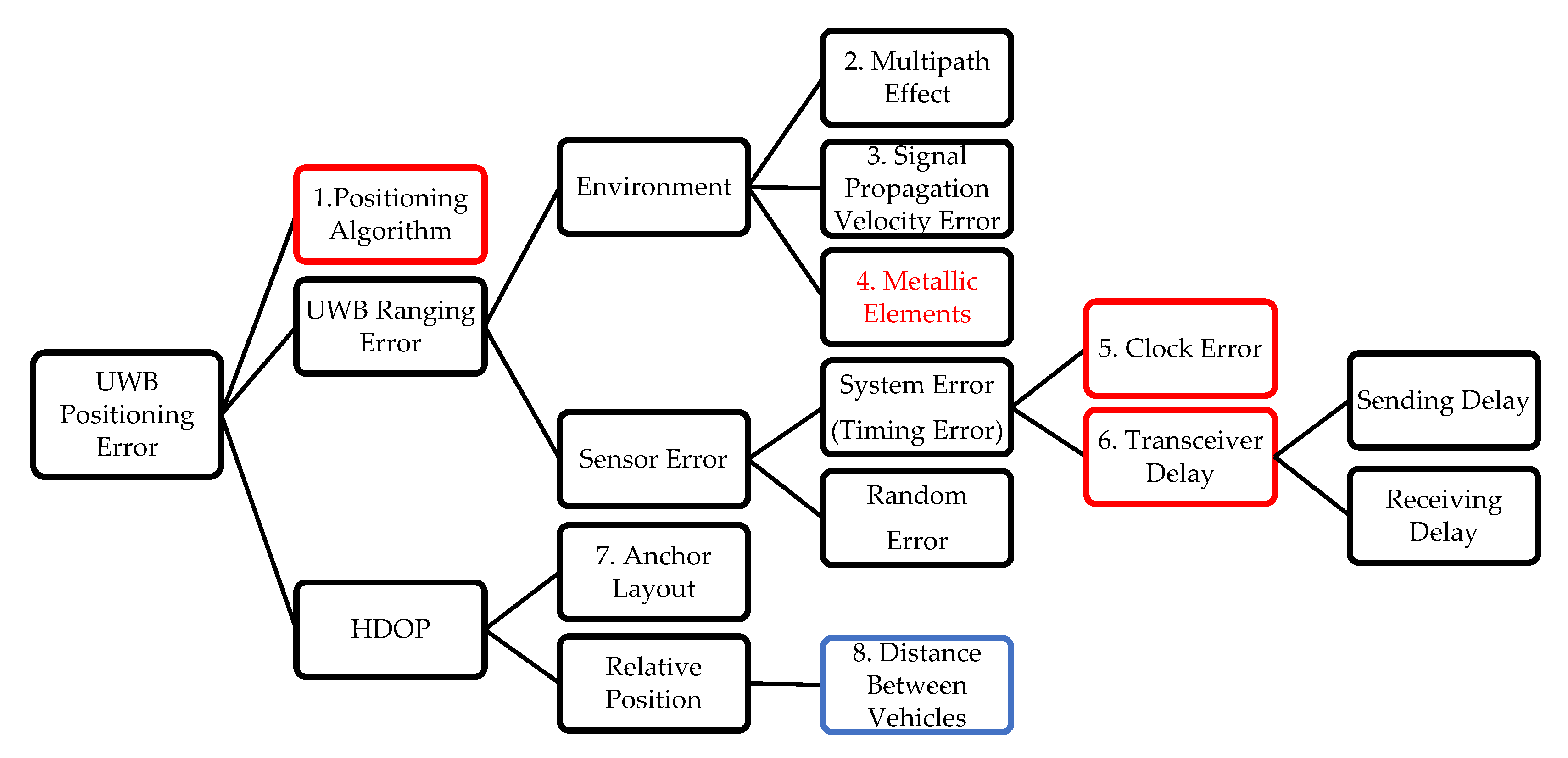
To design a high precision relative localization system, we should first identify the factors that affect the UWB positioning accuracy. Figure 1 shows multiple sources of the UWB positioning error.

As shown in Figure 1, the UWB positioning error is determined by seven factors.

• The positioning algorithm has profound implications for positioning precision.
• The multipath effect error can be easily identified due to the high temporal resolution of UWB signals.
• The signal propagation velocity in the air is almost constant.
• Metallic elements will affect the UWB systems that range using received signal strength indicators (RSSI) [35]. The proposed system, which range using time of flight (TOF), will not encounter this problem.
• The clock error is one of the most critical factors to the ranging accuracy. In the UWB system, the distance is calculated by multiplying the time of flight (TOF) of a UWB signal from a module to another by the speed of light, which means one nanosecond clock error will lead to a 30 cm ranging error.
• The transceiver delay, including sending and receiving delay, is also reflected as a timing error and has a similar effect as the clock error.
• The anchor layout cannot be significantly adjusted in the proposed system, limited by the space on top of the vehicle.
• The distance between two vehicles depends on the particular driving scenarios and is not determined by the system.

Therefore, the factors that need to be considered while designing the system consist of positioning algorithm and timing error, including clock error and antenna delays. In this section, an improved HOMO-LM positioning algorithm is proposed, and a timing error self-correction method is presented. Vehicle positioning is usually not completed in only one way but through multi-sensor integration. For extending the application value of the proposed UWB system, we establish a simple UWB/DR fusion system to validate its contribution to the fusion accuracy.

2.1. UWB Relative Planar Localization Algorithm

2.1.1. The Classic Triangulation Algorithm

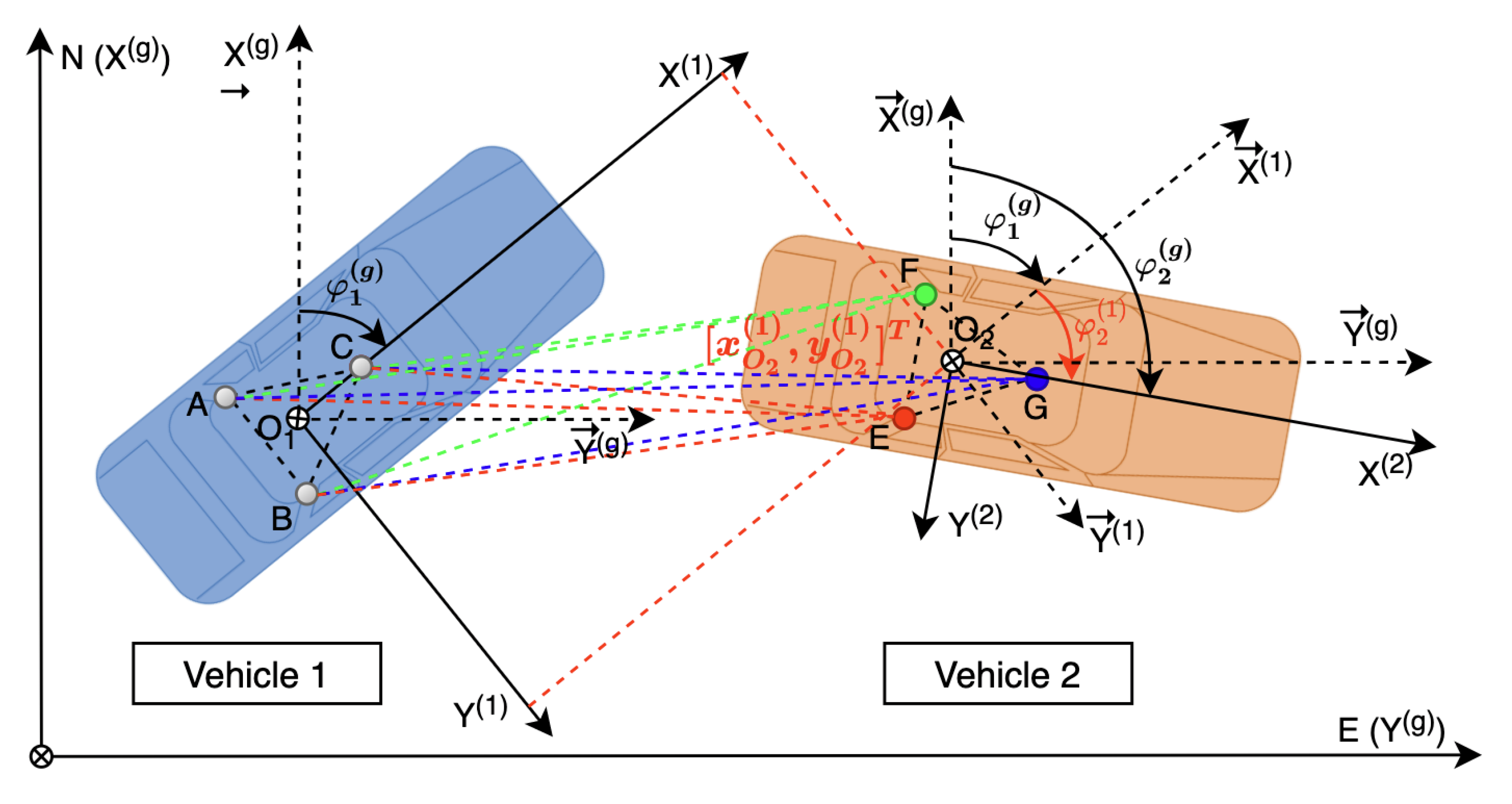
The positioning and directing model is shown in Figure 2. Three UWB modules are installed on the roof of each vehicle. A, B, and C represent the UWB modules on vehicle 1, while E, F, and G represent those on vehicle 2. $O_1$ and $O_2$ represent the centroids of the two vehicles. We define $X_K^{\left(g\right)}={\left[x_K^{\left(g\right)},y_K^{\left(g\right)}\right]}^T$ as the position of point K under the global coordinates system, where $K=\left(A, B, C, E, F, G, O_1, O_2\right)$. ${\phi }_i^{\left(g\right)}$ denotes the heading angle of vehicle $i$ under the global coordinates system, where $i=\left(1, 2\right)$. Similarly, $X_K^{\left(1\right)}={\left[x_K^{\left(1\right)},y_K^{\left(1\right)}\right]}^T$ and ${\phi }_i^{\left(1\right)}$ denote the position and orientation under the coordinate system of vehicle 1. $X_K^{\left(2\right)}={\left[x_K^{\left(2\right)},y_K^{\left(2\right)}\right]}^T$ and ${\phi }_i^{\left(2\right)}$ denote the position and orientation under the coordinate system of vehicle 2.

After the UWB modules were installed, $X_A^{\left(1\right)}$, $X_B^{\left(1\right)}$, $X_C^{\left(1\right)}$, $X_{O_1}^{\left(1\right)}$, $X_D^{\left(2\right)}$, $X_E^{\left(2\right)}$, $X_F^{\left(2\right)}$ and $X_{O_2}^{\left(2\right)}$ were confirmed. UWB measures distances between modules on vehicle 1 and those on vehicle 2. $D_{j,k}$ denotes the distance between module j and module k, where $j=\left(A, B, C\right)$ and $k=\left( E, F, G\right)$. In the proposed system, what we want to know is the relative position $X_{O_2 }^{\left(1\right)}$ and the relative orientation ${\phi }_2^{\left(1\right)}$. Equation (1) can be established using the known parameters;

$$D_{j,k}=\parallel X_j^{\left(1\right)}-X_k^{\left(1\right)}\parallel , \left(j=A,B,C; k=E,F,G\right)$$

(1)

$X_{E }^{\left(1\right)}$, $X_{F }^{\left(1\right)}$, $X_{G }^{\left(1\right)}$ can be solved from (1), as shown in (2).

$$X_{k }^{\left(1\right)}=P^{-1}{N}_k,\left(k=E,F,G\right)$$

(2)

where

$$\begin{array}{l}P=2{\left[X_{\mathrm{B}}^{(1)}-X_{\mathrm{A}}^{(1)},X_{\mathrm{C}}^{(1)}-X_{\mathrm{B}}^{(1)}\right]}^T,\\ N_k=\left[\begin{array}{c}{D}_{A,k}^2-D_{B,k}^2-{∥X_{\mathrm{A}}^{(1)}∥}^2+{∥X_{\mathrm{B}}^{(1)}∥}^2\\ D_{B,k}^2-D_{C,k}^2-{∥X_{\mathrm{B}}^{(1)}∥}^2+{∥X_{\mathrm{C}}^{(1)}∥}^2\end{array}\right].\end{array}$$

Then ${\phi }_2^{\left(1\right)}$ can be derived by (3).

$${\phi }_2^{\left(1\right)}=\frac{1}{3}{\displaystyle \sum }_{j,k}\left[\mathrm{atan}2\left(y_j^{\left(1\right)}-y_k^{\left(1\right)},x_j^{\left(1\right)}-x_k^{\left(1\right)}\right)-\mathrm{atan}2\left(y_j^{\left(2\right)}-y_k^{\left(2\right)},x_j^{\left(2\right)}-x_k^{\left(2\right)}\right)\right],\left(j,k=E,F;F,G;E,G\right)$$

(3)

where,

$$\begin{gathered} \mathrm{atan}2\left(y,x\right)=\mathrm{sgn}{\left(x\right)}^2\arctan \left(\frac{y}{x}\right)+\frac{1-\mathrm{sgn}\left(x\right)}{2}\left(1+\mathrm{sgn}\left(y\right)-\mathrm{sgn}{\left(y\right)}^2\right)\pi , \\ \mathrm{sgn}\left(x\right)=\{\begin{array}{c}\begin{array}{cc}1& x>0\end{array}\\ \begin{array}{cc}0& x=0\end{array}\\ \begin{array}{cc}-1& x<0\end{array}\end{array}. \end{gathered}$$

$X_{O_2 }^{\left(1\right)}$ can be derived by (4);

$$X_{O_2 }^{\left(1\right)}=\overline{X_{EFG}^{\left(1\right)}}-R\overline{X_{EFG}^{\left(2\right)}}$$

(4)

where

$$R=\left[\begin{array}{cc}\cos \left({\phi }_2^{\left(1\right)}\right)& -\sin \left({\phi }_2^{\left(1\right)}\right)\\ \sin \left({\phi }_2^{\left(1\right)}\right)& \cos \left({\phi }_2^{\left(1\right)}\right)\end{array}\right].$$

The overlines represent the mean values of the coordinates of the three modules, such that:

$$\overline{X_{EFG}^{\left(1\right)}}=\frac{1}{3}{\displaystyle \sum }_k{X}_k^{\left(1\right)} \left(k=E,F,G\right), \overline{X_{EFG}^{\left(2\right)}}=\frac{1}{3}{\displaystyle \sum }_k{X}_k^{\left(2\right)} \left(k=E,F,G\right).$$

2.1.2. An Improved HOMO-LM Localization Algorithm

According to the error distribution of triangulation, the positioning and directing error of the classic triangulation method will be extensive when two vehicles are far away. Therefore, an improved HOMO-LM method is proposed for better solutions.

With $X_{E }^{\left(1\right)}$, $X_{F }^{\left(1\right)}$, $X_{G }^{\left(1\right)}$ derived from (2), the side lengths of triangle ${△}_{EFG}$, i.e., $D_{E,F}$, $D_{F,G}$, and $D_{G,E}$ can be calculated by

$$D_{i,j}=\parallel X_i^{\left(1\right)}-X_j^{\left(1\right)}\parallel \left(j,k=E,F;F,G;E,G\right)$$

(5)

However, the real side lengths, $D_{E,F}$, $D_{F,G}$, and $D_{E,G}$ are determined by $X_{E }^{\left(2\right)}$, $X_{F }^{\left(2\right)}$, $X_G^{\left(2\right)}$, as shown in (6).

$$D_{i,j}^{real}=\parallel X_i^{\left(2\right)}-X_j^{\left(2\right)}\parallel \left(j,k=E,F;F,G;E,G\right)$$

(6)

Since ranging error always exists, $D_{E,F}^{real}\ne D_{E,F}$, $D_{F,G}^{real}\ne D_{F,G}$, and $D_{G,E}^{real}\ne D_{G,E}$.

For more accurate solutions, (5) and (6) can be combined as a constraint, i.e., triangular side length constraint, as shown in (7).

$$\{\begin{array}{c}\parallel X_E^{\left(2\right)}-X_F^{\left(2\right)}\parallel -\parallel X_E^{\left(1\right)}-X_F^{\left(1\right)}\parallel =0\\ \parallel X_F^{\left(2\right)}-X_G^{\left(2\right)}\parallel -\parallel X_F^{\left(1\right)}-X_G^{\left(1\right)}\parallel =0\\ \parallel X_E^{\left(2\right)}-X_G^{\left(2\right)}\parallel -\parallel X_E^{\left(1\right)}-X_G^{\left(1\right)}\parallel =0\end{array}$$

(7)

Combining (1) and (7), function $p$ can be established:

$$p(x)=\left[\begin{array}{c}{D}_{AE}-∥X_A^{(1)}-X_E^{(1)}∥\\ D_{BE}-∥X_B^{(1)}-X_E^{(1)}∥\\ D_{CE}-∥X_C^{(1)}-X_E^{(1)}∥\\ D_{AF}-∥X_A^{(1)}-X_F^{(1)}∥\\ D_{BF}-∥X_B^{(1)}-X_F^{(1)}∥\\ D_{CF}-∥X_C^{(1)}-X_F^{(1)}∥\\ D_{AG}-∥X_A^{(1)}-X_G^{(1)}∥\\ D_{BG}-∥X_B^{(1)}-X_G^{(1)}∥\\ D_{CG}-∥X_C^{(1)}-X_G^{(1)}∥\\ ∥X_E^{(2)}-X_F^{(2)}∥-∥X_E^{(1)}-X_F^{(1)}∥\\ ∥X_F^{(2)}-X_G^{(2)}∥-∥X_F^{(1)}-X_G^{(1)}∥\\ ∥X_E^{(2)}-X_G^{(2)}∥-∥X_E^{(1)}-X_G^{(1)}∥\end{array}\right]=0$$

(8)

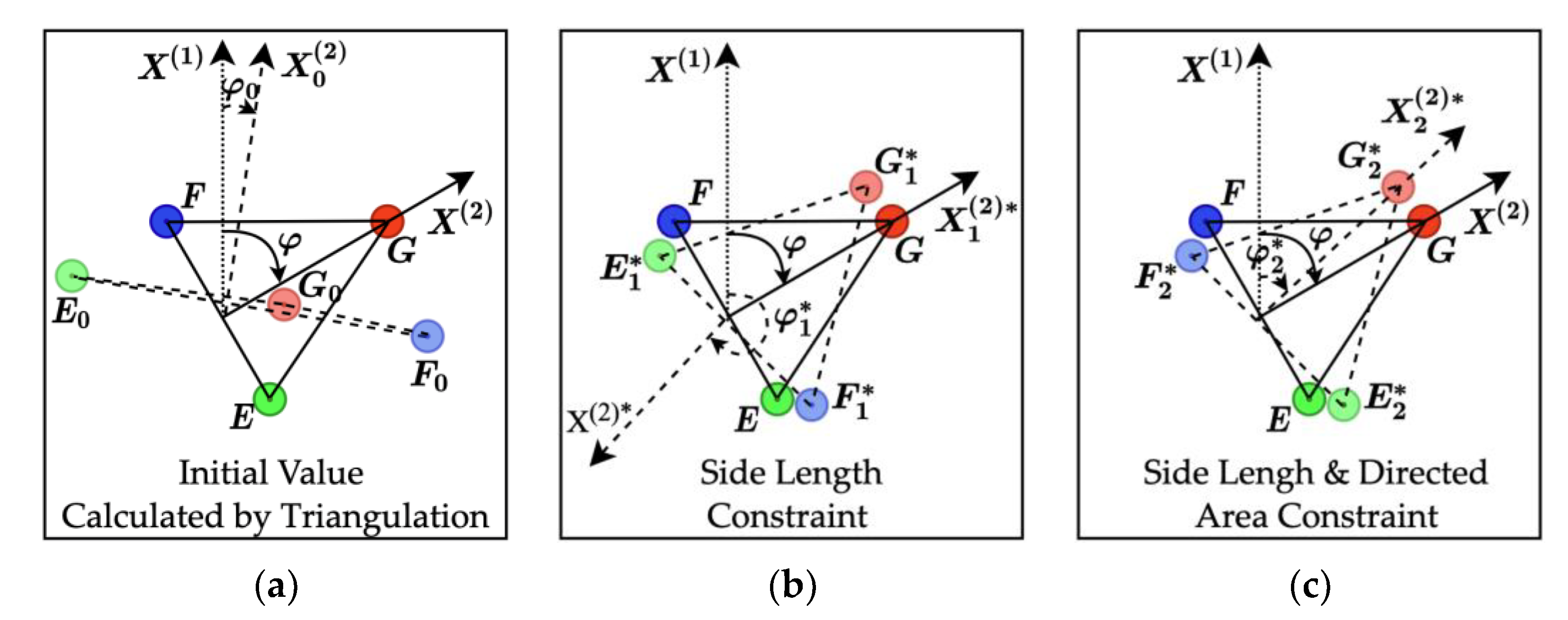
The least-square (LS) solution of (8) will be more accurate than the solution of (2). However, as the positioning error grows extensive, the triangle composed of E, F, and G may flip. The LS solution of (8) will also encounter significant directing errors, as shown in Figure 3. ${△}_{EFG}$ represents the real triangle determined by the real relative positions of module E, F, and G. ${△}_{E_0{F}_0{G}_0}$ represents the triangle determined by the relative positions of module E, F, and G calculated by (2). ${△}_{E_1^{*}{F}_1^{*}{G}_1^{*}}$ represents the triangle determined by the relative positions of module E, F, and G derived from (8). ${△}_{E_2^{*}{F}_2^{*}{G}_2^{*}}$ represents the triangle determined by the relative positions of module E, F, and G derived from (11). φ denotes the real relative orientation. ${\phi }_0$, ${\phi }_1^{*}$, and ${\phi }_2^{*}$ denote the relative orientations determined by ${△}_{E_0{F}_0{G}_0}$, ${△}_{E_1^{*}{F}_1^{*}{G}_1^{*}}$, and ${△}_{E_2^{*}{F}_2^{*}{G}_2^{*}}$, respectively.

As shown in Figure 3a, because of the large positioning error of the classic triangulation method, the triangle ${△}_{E_0{F}_0{G}_0}$, which is constructed by the calculated module coordinates, is seriously deformed. E, F, and G were originally arranged clockwise, but become counterclockwise under the influence of positioning errors. Therefore, the corresponding relative orientation is apparently inaccurate. The shape of the triangle ${△}_{E_1^{*}{F}_1^{*}{G}_1^{*}}$, which is constructed by the LS solutions of (8) with the side length constraint, is similar to the real triangle ${△}_{EFG}$. However, the rotation direction of the three points was still opposite to the real situation, which means that the triangle flipped, as shown in Figure 3b. The error of relative orientation was still large.

The side length constraint cannot deal with this issue. To suppress the triangle flipping, another constraint, i.e., directed area constraint, is necessary. As shown in Figure 3c, with the introduction of the directed area constraint, both the shape and the direction of ${△}_{E_2^{*}{F}_2^{*}{G}_2^{*}}$ are approximate to the real triangle ${△}_{EFG}$. Therefore, the relative orientation is much more accurate. Equation (9) is established to express the directed area constraint.

$$\mathrm{S}\left({△}_{EFG}^{\left(2\right)}\right)-\mathrm{S}\left({△}_{EFG}^{\left(1\right)}\right)=0$$

(9)

where S represents the directed area of the triangle, as shown in (10).

$$\mathrm{S}\left({\mathrm{△}}_{EFG}^{(2)}\right)=\frac{1}{2}\left|\begin{array}{ccc}{\chi }_E^{(2)}& x_F^{(2)}& x_G^{(2)}\\ y_E^{(2)}& y_F^{(2)}& y_G^{(2)}\\ 1& 1& 1\end{array}\right|,\mathrm{s}\left({\mathrm{\Delta }}_{EFG}^{(1)}\right)=\frac{1}{2}\left|\begin{array}{ccc}{x}_E^{(1)}& x_F^{(1)}& x_G^{(1)}\\ y_E^{(1)}& y_F^{(1)}& y_G^{(1)}\\ 1& 1& 1\end{array}\right|.$$

(10)

The directed area is a signed area, which can also be described as half the cross products of triangular edge-vectors. According to the basic properties of the cross product, its sign indicates the rotation direction of the triangle vertices. It should be noted that (9) not only limits the triangle flip but also further constrains the triangle shape. Combining (1), (7), and (9), function $l$ is established:

$$L=l(x)=\left[\begin{array}{c}{D}_{AE}-∥X_A^{(1)}-X_E^{(1)}∥\\ D_{BE}-∥X_B^{(1)}-X_E^{(1)}∥\\ D_{CE}-∥X_C^{(1)}-X_E^{(1)}∥\\ D_{AF}-∥X_A^{(1)}-X_F^{(1)}∥\\ D_{BF}-∥X_B^{(1)}-X_F^{(1)}∥\\ D_{CF}-∥X_C^{(1)}-X_F^{(1)}∥\\ D_{AG}-∥X_A^{(1)}-X_G^{(1)}∥\\ D_{BG}-∥X_B^{(1)}-X_G^{(1)}∥\\ D_{CG}-∥X_C^{(1)}-X_G^{(1)}∥\\ ∥X_E^{(2)}-X_F^{(2)}∥-∥X_E^{(1)}-X_F^{(1)}∥\\ ∥X_F^{(2)}-X_G^{(2)}∥-∥X_F^{(1)}-X_G^{(1)}∥\\ ∥X_E^{(2)}-X_G^{(2)}∥-∥X_E^{(1)}-X_G^{(1)}∥\\ \det \left({\mathrm{\Delta }}_{EFG}^{(2)}\right)-\det \left({\mathrm{\Delta }}_{EFG}^{(1)}\right)\end{array}\right]=0$$

(11)

where $x={\left[x_E^{\left(1\right)},y_E^{\left(1\right)},x_F^{\left(1\right)},y_F^{\left(1\right)},x_G^{\left(1\right)},y_G^{\left(1\right)}\right]}^T.$

Define $x^{*}={\left[x_E^{\left(1\right)*},y_E^{\left(1\right)*},x_F^{\left(1\right)*},y_F^{\left(1\right)*},x_G^{\left(1\right)*},y_G^{\left(1\right)*}\right]}^T$ as the LS solution of (11). Then $x^{*}$ satisfy

$$x^{*}=\mathrm{argmin}(\parallel L\parallel ).$$

(12)

The localization problem can be transformed into a nonlinear least square (NLLS) optimization problem. To address this problem, a HOMO-LM algorithm is proposed in this section. The LM method is an improved Gauss-Newton (GN) and gradient descent (GD) method. LM method has a faster convergence rate than the GD method and can solve the problem with a singular Jacobian matrix, whereas the GN method cannot. To further improved the convergence rate, we integrated the LM method with the Armijo search [36]. The optimized objective function is $l$, which has been defined in (11). The initial value $x_0$ is solved by (2). Define $J_L$ as the Jacobian matrix of function $l$, which can be expressed as shown in (13).

$$J_L=\frac{\partial l}{\partial x}=\left[\begin{array}{ccc}{J}_E& 0& 0\\ 0& J_F& 0\\ 0& 0& J_G\\ J_{EF{G}_1}& J_{EF{G}_2}& J_{EF{G}_3}\end{array}\right]$$

(13)

where

$$\begin{array}{r}{J}_i=\left[\begin{array}{c}\frac{x_A^{(1)}-x_i^{(1)}}{∥X_A^{(1)}-X_i^{(1)}∥}\frac{y_A^{(1)}-y_i^{(1)}}{∥X_A^{(1)}-X_i^{(1)}∥}\\ \frac{x_B^{(1)}-x_i^{(1)}}{∥X_B^{(1)}-X_i^{(1)}∥}\frac{y_B^{(1)}-y_i^{(1)}}{∥X_B^{(1)}-X_i^{(1)}∥}\\ \frac{x_C^{(1)}-x_i^{(1)}}{∥X_C^{(1)}-X_i^{(1)}∥}\frac{y_C^{(1)}-y_i^{(1)}}{∥X_C^{(1)}-X_i^{(1)}∥}\end{array}\right](i=E,F,G),J_{EF{G}_1}=\left[\begin{array}{cc}\frac{x_F^{(1)}-x_E^{(1)}}{∥X_F^{(1)}-X_E^{(1)}∥}& \frac{y_F^{(1)}-y_E^{(1)}}{∥X_F^{(1)}-X_E^{(1)}∥}\\ \frac{x_G^{(1)}-x_E^{(1)}}{∥X_G^{(1)}-X_E^{(1)}∥}& \frac{y_G^{(1)}-y_E^{(1)}}{∥X_G^{(1)}-X_E^{(1)}∥}\\ \frac{y_G^{(1)}-y_F^{(1)}}{2}& \frac{x_F^{(1)}-x_G^{(1)}}{2}\end{array}\right],\\ J_{EF{G}_2}=\left[\begin{array}{cc}\frac{x_E^{(1)}-x_F^{(1)}}{∥X_E^{(1)}-X_F^{(1)}∥}& \frac{y_E^{(1)}-y_F^{(1)}}{∥X_E^{(1)}-X_F^{(1)}∥}\\ \frac{x_G^{(1)}-x_F^{(1)}}{∥X_G^{(1)}-X_F^{(1)}∥}& \frac{y_G^{(1)}-y_F^{(1)}}{∥X_G^{(1)}-X_F^{(1)}∥}\\ 0& 0\\ \frac{y_E^{(1)}-y_G^{(1)}}{2}& \frac{x_G^{(1)}-x_E^{(1)}}{2}\end{array}\right],J_{EF{G}_{\mathfrak{g}}}=\left[\begin{array}{c}\frac{10}{1)}\\ \frac{x_F^{(1)}-x_G^{(1)}}{∥X_F^{(1)}-X_G^{(1)}∥}& \frac{y_F^{(1)}-y_G^{(1)}}{∥X_F^{(1)}-X_G^{(1)}∥}\\ \frac{x_E^{(1)}-x_G^{(1)}}{∥X_E^{(1)}-X_G^{(1)}∥}& \frac{x_E^{(1)}-x_G^{(1)}}{∥X_E^{(1)}-X_G^{(1)}∥}\\ \frac{y_F^{(1)}-y_E^{(1)}}{2}& \frac{x_E^{(1)}-x_F^{(1)}}{2}\end{array}\right].\end{array}$$

Let ε denotes the iteration termination threshold of the optimization algorithm. Define $\rho , \sigma \in \left(0,1\right)$ as the regulatory factors of the Armijo search, μ as the regulatory factor of the LM method. Assume $k_{max}$ and $m_{max}$ as the maximum iterations of the LM method and the Armijo search, respectively.

Table 1. The pseudocode of the LM algorithm with the Armijo search.

Step	Pseudocode
Step 1	Define $L=l\left(x\right)$ as (11) and $J_L=\frac{\partial l}{\partial X}$ as (13);
Step 2	Set $\epsilon ={10}^{-4}, k_{max}=200$, $\rho =0.5, \sigma =0.5,m_{max}=20$;
Step 3	Compute the initial value $x_0={\left[{X_E^{\left(1\right)}}^T,{X_F^{\left(1\right)}}^T,{X_G^{\left(1\right)}}^T\right]}^T$ by (2); Set $x_0^{*}=x_0$; ${\mu }_0=\parallel x_0\parallel$;
Step 4	$k=0$;
Step 5	while $\left(k<k_{\max }\right)$ do
Step 6	Compute $L_k=l\left(x_k\right)$, $J_{L_k}$;
Step 7	$g_k=J_{L_k}^T{L}_k$; $d_k={\left(-J_{L_k}^T{J}_{L_k}+{\mu }_{k}I\right)}^{-1}{g}_k$;
Step 8	if $\parallel g_k\parallel <\epsilon$ do     break;   end if
Step 9	$m=0$;   while ($m<m_{max})$ do     if $\left(\parallel l\left(x_k+{\rho }^m{d}_k\right)\parallel <\parallel l\left(x_k\right)\parallel +\sigma {\rho }^m{g}_k^T{d}_k\right)$ do       $m=m+1$;     end if   end while   $\alpha ={\rho }^m$;
Step 10	$x_{k+1}=x_k+\alpha d_k$;
Step 11	$k=k+1$;
Step 12	${\mu }_k=\parallel x_k\parallel$;
Step 13	end while
Step 14	$x^{*}=x_k$;
Step 15	Output $x^{*}$as the optimal solution of equation$l\left(x\right)=0$

shows the pseudocode of the LM method with the Armijo search.

Like many other fitting algorithms, the optimization result of the LM method relies on the initial value. LM may only find a local minimum instead of the global minimum or even diverge without the proper initial value. The positioning error increases with the increase of the distance between two vehicles, which also means the error of the initial value $x_0$ increases. Therefore, the homotopy method is introduced for searching for an optimal initial value in a broader range. Assume $f\left(x\right)=0$ is the equation we want to solve, and $f_0$ is a known function with an available zero solution $x^{*}$, i.e., $f_0\left(x^{*}\right)=0.$ We conduct a depending parameter function

$$h\left(x,s\right)=sf\left(x\right)+\left(1-s\right)f_0\left(x\right) s\in \left[0,1\right].$$

(14)

$h\left(x,0\right)=0$ is the problem with a known solution $x^{*}$, and $H\left(x,1\right)=0$ is the original problem $f\left(x\right)=0$.

In the proposed system, we define $f\left(x\right)=l\left(x\right)$, $f_0\left(x\right)=l\left(x\right)-l\left(x^{*}\right)$. This gives the homotopy function

$$H=h\left(x,s\right)=l\left(x\right)+\left(s-1\right)l\left(x^{*}\right) s\in \left[0,1\right].$$

(15)

As the solution of $h\left(x,s\right)=0$ depends on $s$, we denote it by $x^{*}\left(s\right)$. $s$ can be discretized into $0=s_0<s_1<s_2<···<s_n=1$. Then the optimization of (11) can be transformed into solving a sequence of nonlinear equations with the LM method such that

$$h\left(x,s_i\right)=0.$$

(16)

Each iteration is started with the solution $x^{*}\left(s_{i-1}\right)$.

Table 2. The pseudocode of the HOMO-LM algorithm.

Step	Pseudocode
Step 1	Define $L=l\left(x\right)$ as (11) and derive $J_L$=$\frac{\partial l}{\partial X}$ as (13); Define $H=h\left(x,s,x^{*}\right)=l\left(x\right)+\left(s-1\right)l\left(x^{*}\right)$ and $J_H=J_L$;
Step 2	Set $\epsilon ={10}^{-4}, k_{max}=200,s_0=0, \Delta s=0.1, s_{end}=1,\rho =0.5, \sigma =0.5,$$m_{max}=20$;
Step 3	Compute the initial value $x_0={\left[{X_E^{\left(1\right)}}^T,{X_F^{\left(1\right)}}^T,{X_G^{\left(1\right)}}^T\right]}^T$ by (2); Set $x_0^{*}=x_0$; ${\mu }_0=\parallel x_0\parallel$;
Step 4	for$n=1:\frac{\left(s_{end}-s_0+\Delta s\right)}{\Delta s}$ do
Step 5	$s_n=s_0+\left(n-1\right)\Delta s$;
Step 6	$k=0$;
Step 7	while $\left(k<k_{\max }\right)$ do
Step 8	Compute $H_k=h\left(x_k,s_n,x_{n-1}^{*}\right)$, $J_{H_k}$;
Step 9	$g_k=J_{H_k}^T{H}_k$; $d_k={\left(-J_{H_k}^T{J}_{H_k}+{\mu }_{k}I\right)}^{-1}{g}_k$;
Step 10	if $\parallel g_k\parallel <\epsilon$ do       break;     end if
Step 11	$m=0$;     while ($m<m\_max)$ do       if $\left(\parallel f\left(x_k+{\rho }^m{d}_k\right)\parallel <\parallel f\left(x_k\right)\parallel +\sigma {\rho }^m{g}_k^T{d}_k\right)$ do         $m=m+1$;       end if     end while     $\alpha ={\rho }^m$;
Step 12	$x_{k+1}=x_k+\alpha d_k$;
Step 13	$k=k+1$;
Step 14	${\mu }_k=\parallel x_k\parallel$;
Step 15	end while
Step 16	$x_n^{*}=x_k$;
Step 17	end for
Step 18	Output $x^{*}=x_n^{*}$as the optimal solution of equation$f\left(x\right)=0$

shows the pseudocode of the proposed HOMO-LM algorithm.

After the LS solution of $x^{*}$ of (2) being calculated, positions of E, F, G are confirmed. Define

$$\begin{gathered} X_{EFG}^{\left(1\right)*}=\left[X_E^{\left(1\right)*},X_F^{\left(1\right)*},X_G^{\left(1\right)*}\right] \\ {X}_{EFG}^{\left(2\right)}=\left[X_E^{\left(2\right)},X_F^{\left(2\right)},X_G^{\left(1\right)}\right] \\ \overline{X_{EFG}^{\left(1\right)*}}=\frac{1}{3}{\displaystyle \sum }_k{X}_k^{\left(1\right)*}, \left(k=E,F,G\right) \\ \overline{X_{EFG}^{\left(2\right)}}=\frac{1}{3}{\displaystyle \sum }_k{X}_k^{\left(2\right)}, \left(k=E,F,G\right) \end{gathered}$$

(17)

Then the LS solutions of the relative position $X_{O_2 }^{\left(1\right)*}$ and orientation ${\phi }_2^{\left(1\right)*}$ can be derived using singular value decomposition (SVD) [37]. Define M as

$$M={\left[X_{EFG}^{\left(2\right)}-\overline{X_{EFG}^{\left(2\right)}}\left[1,1,1\right]\right]}^T\left[X_{EFG}^{\left(1\right)*}-\overline{X_{EFG}^{\left(1\right)*}}\left[1,1,1\right]\right]$$

(18)

Take SVD of M:

$$M=U\mathsf{\Sigma }{V}^T$$

(19)

where U, Σ, and V represent the three decomposed matrixes of M. Then we have

$$R=V{U}^T$$

(20)

$$\{\begin{array}{c}{X}_{O_2}^{\left(1\right)*}=\overline{X_{EFG}^{\left(1\right)*}}-R\overline{X_{EFG}^{\left(2\right)}}\\ {\phi }_2^{\left(1\right)*}=\mathrm{atan}2\left(R_{2,1},R_{1,1}\right)\end{array}$$

(21)

2.2. A UWB Timing Error Self-Correction Method

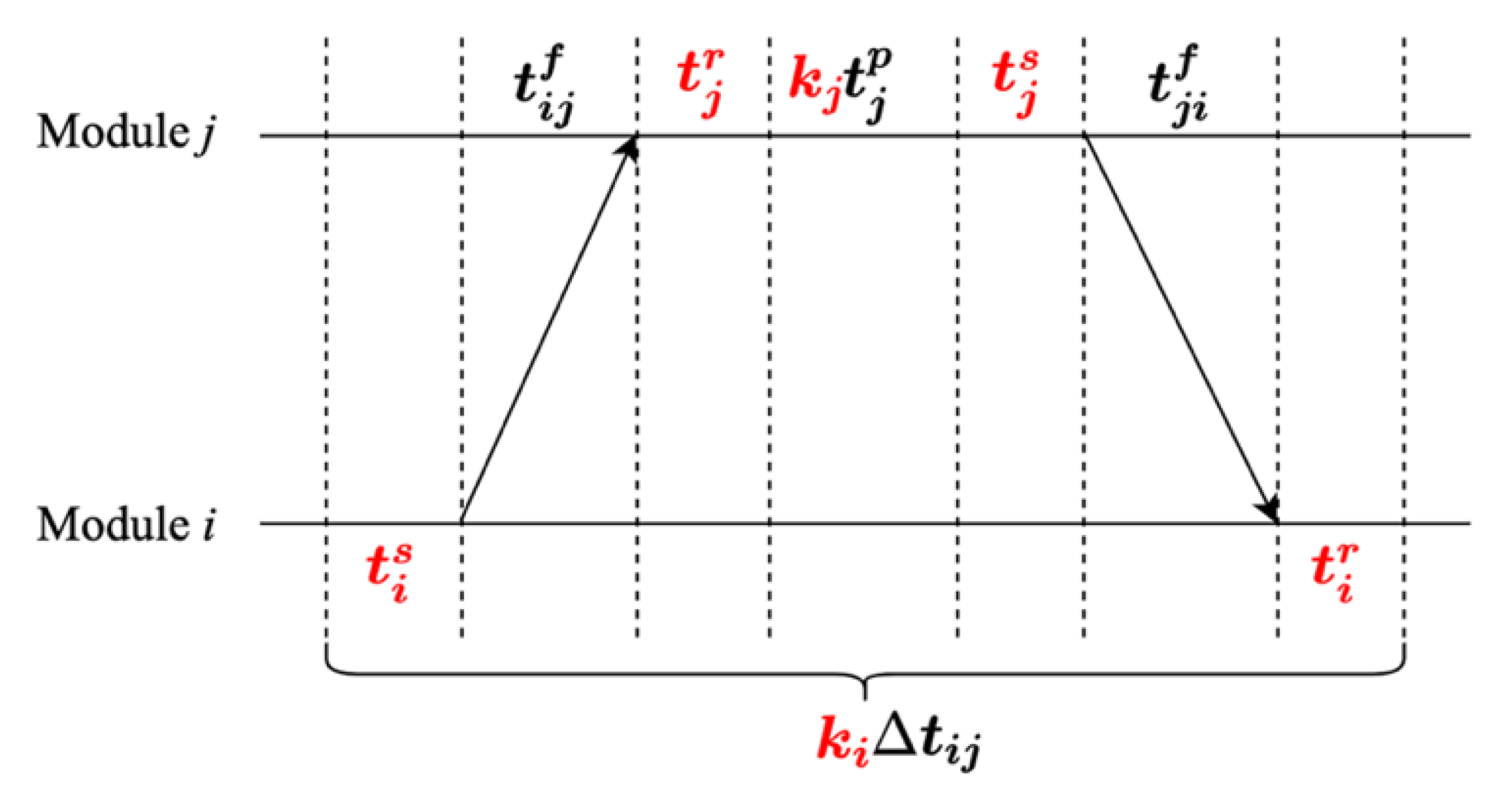
Figure 4 shows the typical two-way ranging (TWR) system. Assume $d_{ij}$ is the original measurement of the distance between module $i$ and $j$ without correction, ${\widehat{d}}_{ij}$ is the corrected measurement and $d_{ij}^{real}$ is the real distance. Other adopted symbols are illustrated in

Table 3. The symbols used in the calibration mode.

Symbols	Title 2
$k_i \left(i=A,B,C\right)$	The clock correction coefficient, which is unknown.
$t_i^s \left(i=A,B,C\right)$	The sending delay of module $i$, which is unknown.
$t_i^r \left(i=A,B,C\right)$	The receiving delay of module $i$, which is unknown.
$t_i^d \left(i=A,B,C\right)$	The antenna delay. $t_i^d=t_i^s+t_i^r$.
$t_i^{p_j} \left(i=A,B,C;j=1,2,3,4\right)$	The time spent by module $i$ from receiving to sending a signal, which is measured by the crystal oscillator inside module $i$. As $t_i^p$ is not a constant, number $j$ is added to distinguish the measurements at different times.
$t_{ij}^f \left(ij=AB,BC,AC\right)$	The signal propagation time from module $i$ to $j$. It is a particular value after modules being installed. That is $t_{ij}^f=\frac{\parallel X_i^{\left(1\right)}-X_j^{\left(1\right)}\parallel }{c}$, where $c$ is the speed of light.
$\Delta t_i^{sr} \left(i=A,B,C\right)$	The interval time from module $i$ sending a signal to receiving a signal, measured by the crystal oscillator inside module $i$.
$\Delta t_i^{rr} \left(i=A,B,C\right)$	The interval time for module $i$ from receiving a signal to another, measured by the crystal oscillator inside module $i$. Number $j$ is added to distinguish the measurements at different times.
$k_i \left(i=A,B,C\right)$	The clock correction coefficient.

. Then we have

$$\begin{gathered} d_{ij}^{real}=c{t}_{ij}^f, \\ {d}_{ij}=\frac{c\left(\Delta t_{ij}-t_j^p\right)}{2}, \\ {\widehat{d}}_{ij}=\frac{c\left(k_i\Delta t_{ij}-k_j{t}_j^p-t_i^s-t_i^r-t_j^s-t_j^r\right)}{2}. \end{gathered}$$

(22)

$d_{ij}$ ignores several important parameters including $t_i^s$, $t_i^r$, $t_j^s$, $t_j^r$, $k^i$ and $k_j$.

UWB modules A, B, and C on vehicle 1 are taken as an example to show the correction process. The symbols used in the correction method are interpreted in Table 3.

Since $t_i^{p_j}$, $\Delta t_i^{sr}$, and $\Delta t_i^{rr}$ are measured by the crystal oscillator inside UWB module $i$, which do not equal the real interval time, because of the crystal oscillation frequency error. The real values are

$$\begin{gathered} {\widehat{t}}_i^{p_j}=k_i{t}_i^{p_j}, \\ \Delta {\widehat{t}}_i^{sr}=k_i\Delta t_i^{sr}, \\ \Delta {\widehat{t}}_i^{rr}=k_i\Delta t_i^{rr}. \end{gathered}$$

(23)

Two calibration modes are designed to implement the correction algorithm, as described as follows.

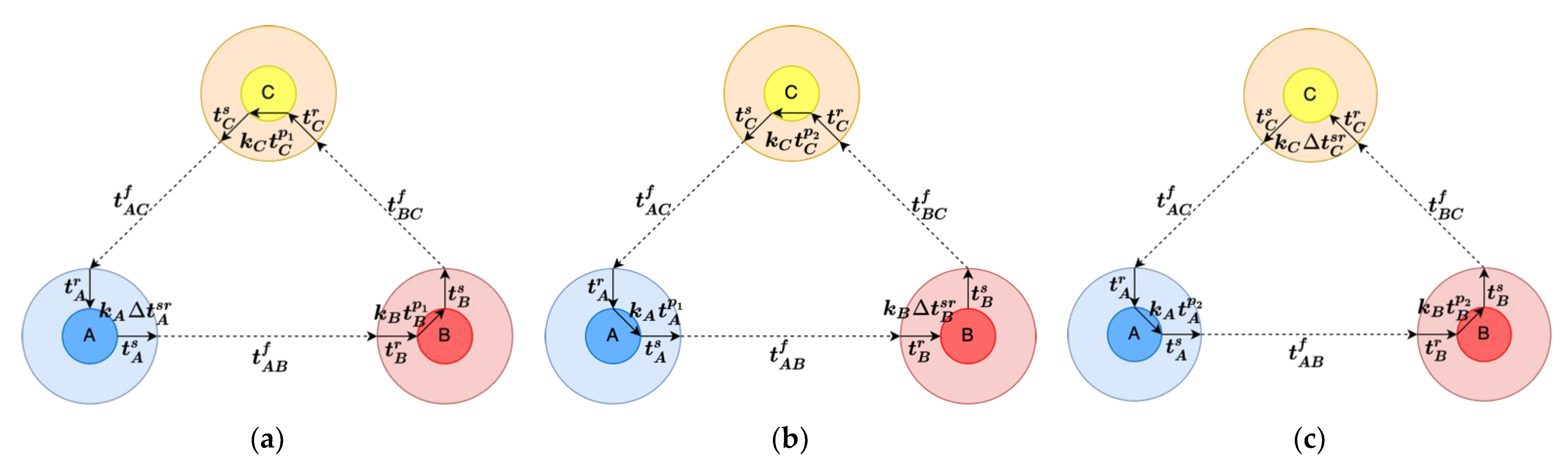
• Circulation Mode: UWB signals transmit among the modules in turn. All the correction parameters are encountered in this mode, as shown in Figure 5.
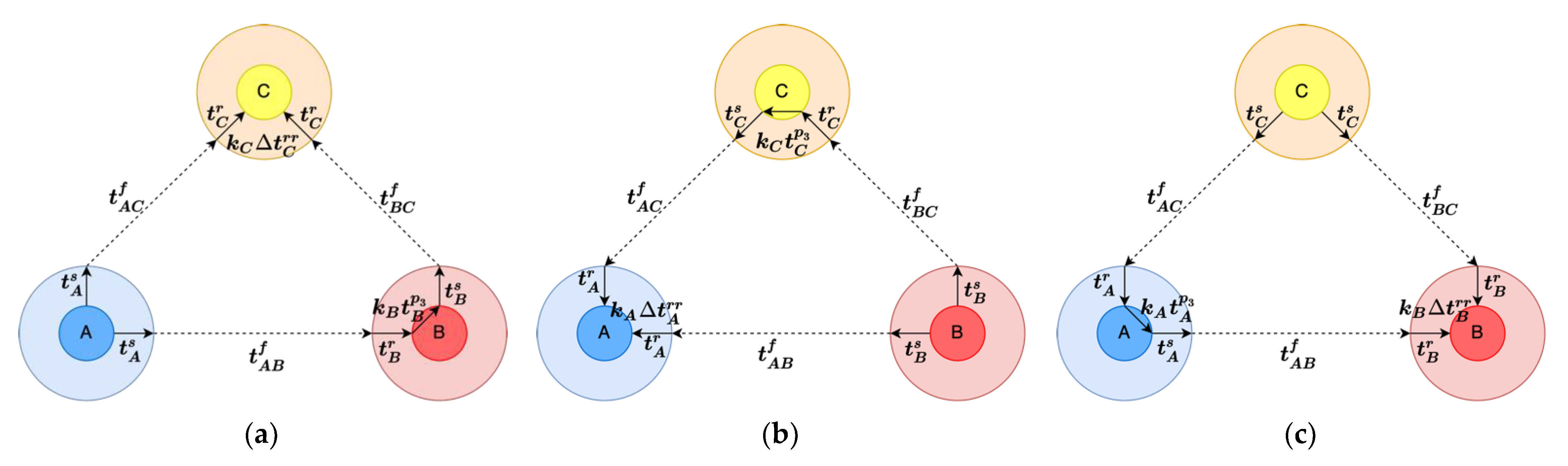
• Differential Mode: UWB signals transmit from a module to another in two paths. The sending delay of the sending module and the receiving delay of the receiving module are eliminated, as shown in Figure 6.

$k_i$ and $t_i^d$ are the parameters needed to correct the ranging error. Equation (24) is established according to the circulation mode;

$$\left\{\begin{array}{l}{k}_A\mathrm{\Delta }{t}_A^{sr}=t_A^s+t_{AB}^f+t_B^r+k_B{t}_B^{p_1}+t_B^s+t_{BC}^f+t_C^r+k_C{t}_C^{p_1}+t_C^s+t_{AC}^f+t_A^r\\ k_B\mathrm{\Delta }{t}_B^{sr}=t_B^s+t_{BC}^f+t_C^r+k_C{t}_C^{p_2}+t_C^s+t_{AC}^f+t_A^r+k_A{t}_A^{p_1}+t_A^s+t_{AB}^f+t_B^r\alpha \\ k_C\mathrm{\Delta }{t}_C^{sr}=t_C^s+t_{AC}^f+t_A^r+k_A{t}_A^{p_2}+t_A^s+t_{AB}^f+t_B^r+k_B{t}_B^{p_2}+t_B^s+t_{BC}^f+t_C^r\end{array}\right.$$

(24)

Equation (25) is established according to the differential mode.

$$\left\{\begin{array}{l}{k}_C\mathrm{\Delta }{t}_C^{r\mathrm{r}}=\left(t_A^s+t_{AB}^f+t_B^r+k_B{t}_B^{p_3}+t_B^s+t_{BC}^f+t_C^r\right)-\left(t_A^s+t_{AC}^f+t_C^r\right)\\ k_A\mathrm{\Delta }{t}_A^{r\mathrm{r}}=\left(t_B^s+t_{BC}^f+t_C^r+k_C{t}_C^{p_3}+t_C^s+t_{AC}^f+t_A^r\right)-\left(t_B^s+t_{AB}^f+t_A^r\right)\\ k_B\mathrm{\Delta }{t}_B^{r{r}_1}=\left(t_C^s+t_{AC}^f+t_A^r+k_A{t}_A^{p_3}+t_A^s+t_{AB}^f+t_B^r\right)-\left(t_C^s+t_{BC}^f+t_B^r\right)\end{array}\right.$$

(25)

Define $t={\left[k_A,k_B,k_C,t_A^d,t_B^d,t_C^d\right]}^T$. Equation (26) can be established combining (24) and (25). $t_i^s$ and $t_i^r$ are eliminated because $t_i^d=t_i^s+t_i^r$, which has been introduced in Table 3.

$$Q_{1}t=\left[\begin{array}{cccccc}\mathrm{\Delta }{t}_A^{sr}& -t_B^{p_1}& -t_c^{p_1}& -1& -1& -1\\ -t_A^{p_1}& \mathrm{\Delta }{t}_B^{sr}& -t_C^{p_2}& -1& -1& -1\\ -t_A^{p_2}& t_B^{p_2}& \mathrm{\Delta }{t}_C^{sr}& -1& -1& -1\\ 0& -t_B^{p_3}& \mathrm{\Delta }{t}_C^{rr}& 0& -1& 0\\ \mathrm{\Delta }{t}_A^{rr}& 0& -t_C^{p_3}& 0& 0& -1\\ -t_A^{p_3}& \mathrm{\Delta }{t}_B^{rr}& 0& -1& 0& 0\end{array}\right]\left[\begin{array}{c}{k}_A\\ k_B\\ k_C\\ t_A^d\\ t_B^d\\ t_C^d\end{array}\right]=\left[\begin{array}{c}{t}_{AB}^f+t_{BC}^f+t_{AC}^f\\ t_{AB}^f+t_{BC}^f+t_{AC}^f\\ t_{AB}^f+t_{BC}^f+t_{AC}^f\\ t_{AB}^f+t_{BC}^f-t_{AC}^f\\ t_{AB}^f-t_{BC}^f+t_{AC}^f\\ -t_{AB}^f+t_{BC}^f+t_{AC}^f\end{array}\right]=b_1$$

(26)

The correction process needs repeating for a while to decrease the influence of random noise. That means

$$Qt={\left[Q_1^T,Q_2^T,\cdots ,Q_n^T\right]}^{T}t={\left[b_1^T,b_2^T,\cdots ,b_n^T\right]}^T=b$$

(27)

Then the LS solution $t^{*}={\left[k_A^{*},k_B^{*},k_C^{*},t^{*}{}_A^s,t^{*}{}_B^s,t^{*}{}_C^s,t^{*}{}_A^r,t^{*}{}_B^r,t^{*}{}_C^r\right]}^T$ of (27) can be expressed as

$$t^{*}={\left(Q^{T}Q\right)}^{-1}{Q}^{T}b.$$

(28)

Besides, we also preprocess the range measurements before positioning to further improve the positioning accuracy. Figure 4 shows a typical two-way ranging system. In fact, the UWB system can range in high frequency up to thousands of times per second. The positioning system does not always need that high data refresh rate. Therefore, we can average multiple measurements, which reduces the interference of random errors without introducing too much latency.

2.3. An Intergrating Model of UWB and DR

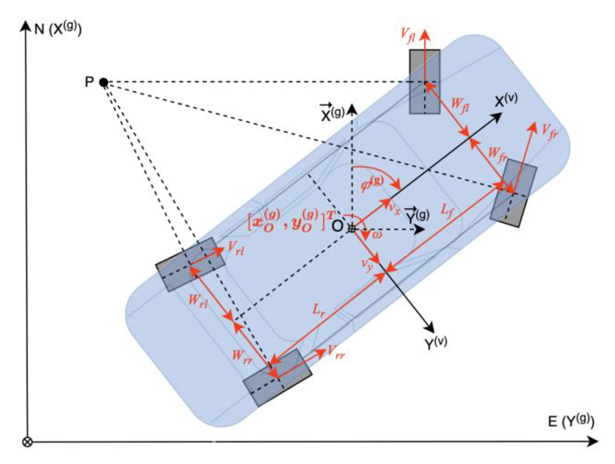
The DR system consists of wheel-speed sensors. Each vehicle is equipped with four wheel-speed sensors. According to the Ackerman steering principle, the instantaneous centers of four wheels coincide at point P, as shown in Figure 7. In the DR model, $v_{fr}$, $v_{fl}$,$v_{rr}$, and $v_{rl}$ are the speeds of the wheels measured by wheel-speed sensors. To obtain the longitudinal velocity $v_x$, lateral velocity $v_y$, and yaw rate $\omega$, (29) can be established.

$$\{\begin{array}{c}{v}_{fr}=\parallel {\left[v_x+\omega W_{fr},v_y+\omega L_f\right]}^T\parallel \\ v_{fl}=\parallel {\left[v_x-\omega W_{fl},v_y+\omega L_f\right]}^T\parallel \\ v_{rr}=\parallel {\left[v_x+\omega W_{rr},v_y-\omega L_r\right]}^T\parallel \\ v_{rl}=\parallel {\left[v_x-\omega W_{rr},v_y-\omega L_r\right]}^T\parallel \end{array}$$

(29)

Equation (29) has a similar form as (11), so the proposed HOMO-LM algorithm in Section 2.1.2 is also suitable here.

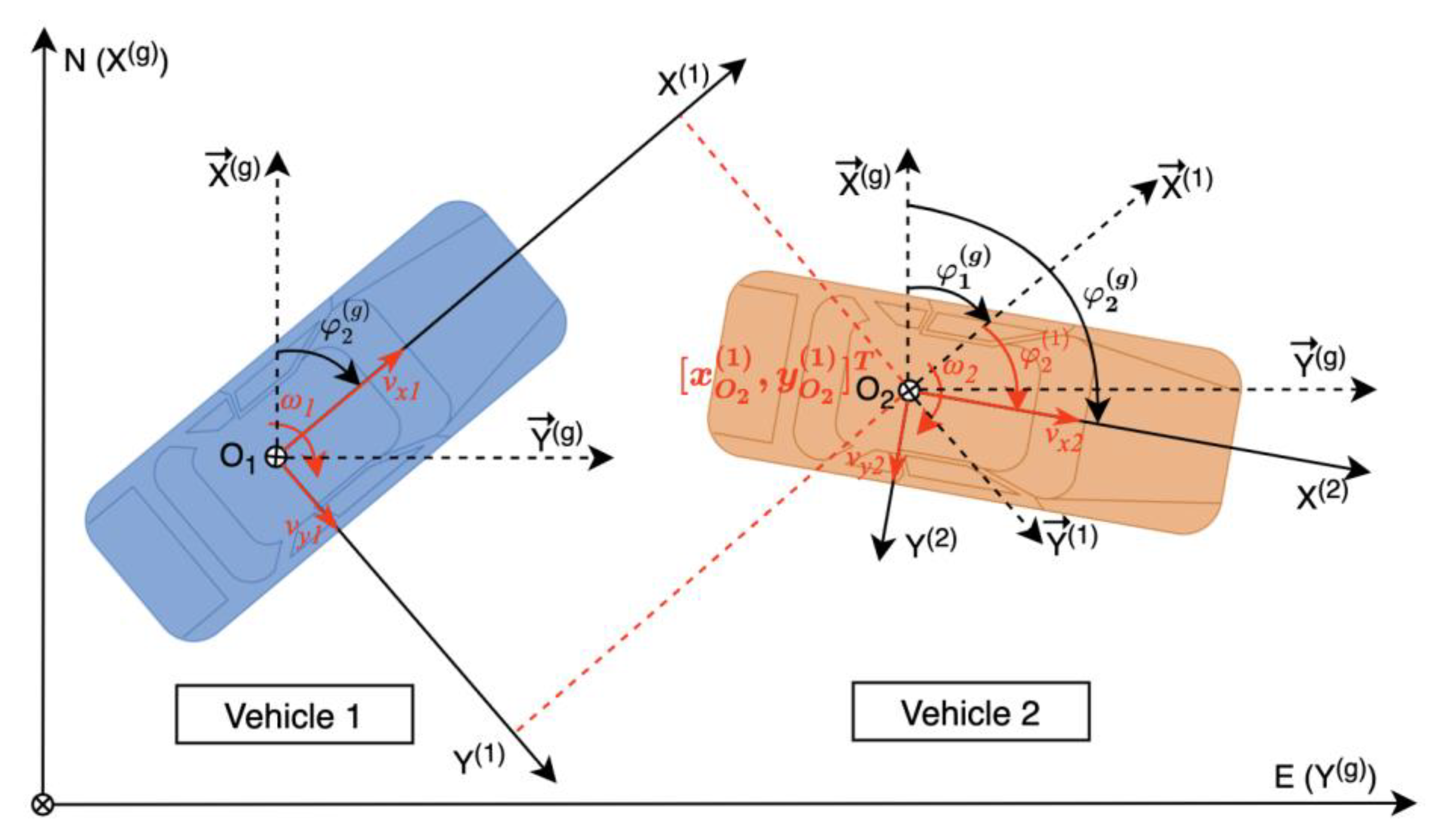
After $v_x$, $v_y$, and $\omega$ solved, the UWB/DR fusion model can be established based on the relative kinematic model shown in Figure 8.

Let $X_k$ denotes the state vector, which contains the relative position and orientation of vehicle 2 in the coordinate system of vehicle 1 ${\left[x_k^{\left(1\right)},y_k^{\left(1\right)},{\phi }_k^{\left(1\right)}\right]}^{\mathrm{T}}$, yaw rates $\left[{\omega }_1{}_k,{\omega }_{2_k}\right]$, and velocities ${\left[v_{x1}{}_k,v_{y1}{}_k,v_{x2}{}_k,v_{y2}{}_k\right]}^T$ of two vehicles. That is

$$X_k={\left[x_k^{\left(1\right)},y_k^{\left(1\right)},{\phi }_k^{\left(1\right)},{\omega }_1{}_k,{\omega }_2{}_k,v_{x_{1}1}{}_k,v_{y1}{}_k,v_{x2}{}_k,v_{y2}{}_k\right]}^T.$$

(30)

The state at time k can be predicted by function $f$ with reference to the state at time k−1. $\Delta t$ denotes the update interval. The state prediction equation can be expressed as

$$X_k=\left[\begin{array}{c}{X}^{\prime }\cos \left({\omega }_{1_{k-1}}\mathrm{\Delta }t\right)+Y^{\prime }\sin \left({\omega }_{1_{k-1}}\mathrm{\Delta }t\right)\\ -X^{\prime }\sin \left({\omega }_{1_{k-1}}\mathrm{\Delta }t\right)+Y^{\prime }\cos \left({\omega }_{1_{k-1}}\mathrm{\Delta }t\right)\\ {\phi }_{k-1}^{(1)}-{\omega }_{1_{k-1}}\mathrm{\Delta }t+{\omega }_{2_{k-1}}\mathrm{\Delta }t\\ {\omega }_{1_{k-1}}+W_{{\omega }_1}\mathrm{\Delta }t\\ {\omega }_{2_{k-1}}+W_{{\omega }_2}\mathrm{\Delta }t\\ v_{x{1}_{k-1}}+W_{v_{x1}}\mathrm{\Delta }t\\ v_{y{1}_{k-1}}+W_{v_{y1}}\mathrm{\Delta }t\\ v_{y{2}_{k-1}}+W_{v_{x2}}\mathrm{\Delta }t\\ v_{x{2}_{k-1}}+W_{v_{y2}}\mathrm{\Delta }t\end{array}\right]$$

(31)

where

$$X^{\prime }=x_{k-1}+v_{x2}{}_{k-1}\cos {\phi }_{k-1}\Delta t-v_{y2}{}_{k-1}\sin {\phi }_{k-1}\Delta t-v_{x1}{}_{k-1}\Delta t,$$

$$Y^{\prime }=y_{k-1}+v_{x2}{}_{k-1}\sin {\phi }_{k-1}\Delta t+v_{y2}{}_{k-1}\cos {\phi }_{k-1}\Delta t-v_{y1}{}_{k-1}\Delta t,$$

$W_{{\omega }_1}$,$W_{{\omega }_2}$,$W_{v_{x1}}$,$W_{v_{y1}}$,$W_{v_{x2}}$, and $W_{v_{y2}}$ denote the noise in the prediction process.

Because all the state values can be measured directly or being calculated, the observation vector is

$$z_k={\left[Z_{x_k^{\left(1\right)}},Z_{y_k^{\left(1\right)}},Z_{{\phi }_k^{\left(1\right)}},Z_{{\omega }_1{}_k},Z_{{\omega }_2{}_k},Z_{v_{x1}{}_k},Z_{v_{y1}{}_k},Z_{v_{x2}{}_k},Z_{v_{y2}{}_k}\right]}^T.$$

(32)

The observation equation can be expressed as

$$z_k=I{X}_k$$

(33)

where $I$ is an identity matrix.

Since the fusion system is nonlinear and the Jacobian matrix of the state prediction equation is complex, the unscented Kalman filter (UKF) [38,39] method has advantages in dealing with this kind of problem. The UKF model is not difficult to build based on (31) and (33), so the process will not be elaborated in this paper.

3. Simulations

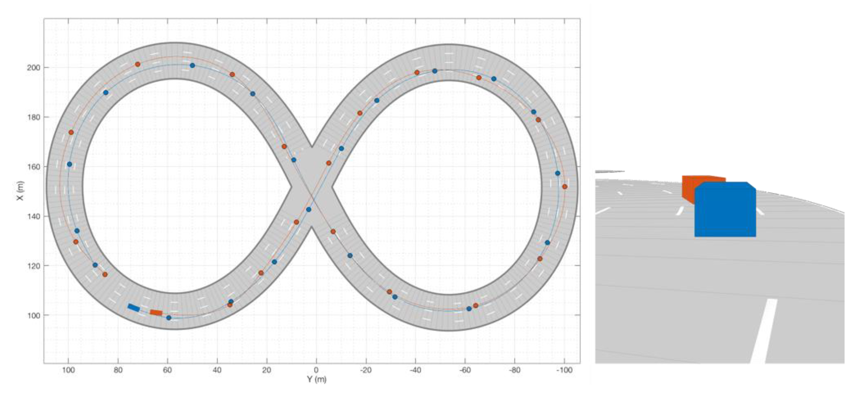
As timing errors cannot be eliminated entirely, we create a virtual environment to validate the feasibility and necessity of the proposed HOMO-LM localization algorithm by simulation, regardless of the influence of clock errors and antenna delays. The driving scenario is established in the Driving Scenario Designer of MATLAB, as shown in Figure 9. The parameter setups of the two vehicles are shown in

Table 4. Parameters of vehicle 1 in the Driving Scenario Designer.

Sequence Number of Waypoints	Coordinate (m)	Velocity (m/s)	Wait Time (s)
1	[103.5; 74.9]	0.0	1.0
2	[99.0; 59.6]	5.0	0.0
3	[105.4; 34.4]	20.0	0.0
4	[121.5; 17.0]	20.0	0.0
5	[142.6; 3.2]	30.0	0.0
6	[167.3; −10.1]	30.0	0.0
7	[186.6; −24.3]	30.0	0.0
8	[198.5; −47.7]	30.0	0.0
9	[195.3; −71.6]	30.0	0.0
10	[182.0; −87.6]	30.0	0.0
11	[157.2; −97.3]	30.0	0.0
12	[129.3; −93.1]	30.0	0.0
13	[102.6; −61.5]	30.0	0.0
14	[107.4; −31.7]	30.0	0.0
15	[124.1; −13.6]	30.0	0.0
16	[162.7; 9.2]	30.0	0.0
17	[189.4; 25.7]	30.0	0.0
18	[200.8; 50.0]	30.0	0.0
19	[189.8; 84.9]	30.0	0.0
20	[160.9; 99.6]	30.0	0.0
21	[134.0; 96.5]	20.0	0.0
22	[120.3; 89.3]	0.0	2.0

and

Table 5. Parameters of vehicle 2 in the Driving Scenario Designer.

Sequence Number of Waypoints	Coordinate (m)	Velocity (m/s)	Wait Time (s)
1	[101.2; 66.0]	0.0	1.0
2	[104.2; 34.9]	10.0	0.0
3	[117.0; 22.4]	15.0	0.0
4	[137.5; 8.1]	20.0	0.0
5	[161.4; −4.9]	20.0	0.0
6	[181.5; −17.6]	20.0	0.0
7	[197.9; −40.5]	40.0	0.0
8	[195.9; −65.5]	30.0	0.0
9	[178.8; −89.5]	30.0	0.0
10	[151.8; −100.2]	30.0	0.0
11	[122.7; −90.1]	30.0	0.0
12	[103.9; −64.2]	30.0	0.0
13	[109.4; −29.5]	50.0	0.0
14	[133.7; −6.8]	30.0	0.0
15	[168.1; 13.0]	30.0	0.0
16	[197.2; 33.9]	30.0	0.0
17	[201.3; 72.0]	30.0	0.0
18	[173.8; 98.9]	30.0	0.0
19	[129.6; 97.0]	30.0	0.0
20	[116.4; 85.2]	0.0	2.0

, respectively. In the Driving Scenario Designer, the coordinates of the waypoints are selected randomly. The velocities of the vehicles can be updated only at the waypoints. The values of velocities are adjusted to avoid vehicle collisions during the simulation. The wait time means the duration that a vehicle stays at a waypoint. The sample interval of the system is set to 0.01 s.

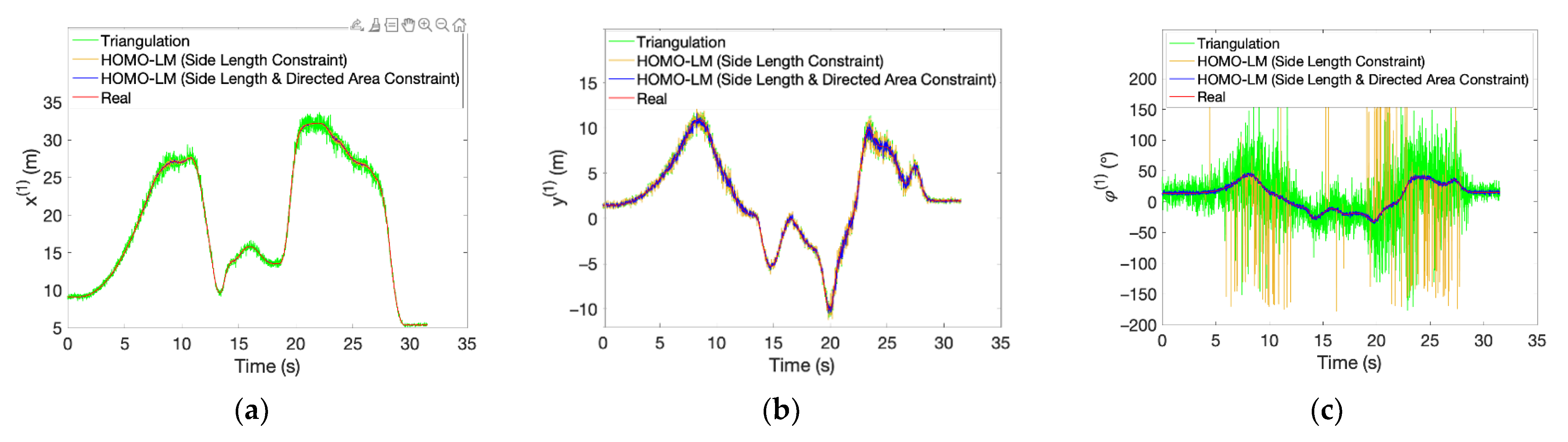
The simulation results are shown in Figure 10. The proposed method significantly improves the longitudinal positioning accuracy, whether with or without the directed area constraint. As for the lateral positioning accuracy, it cannot be improved by the side length constraint alone. Besides, the directing accuracy is improved by the side length constraint in most cases, although some jumping points still exist. All abnormal orientation data is eliminated with the introduction of the directed area constrain.

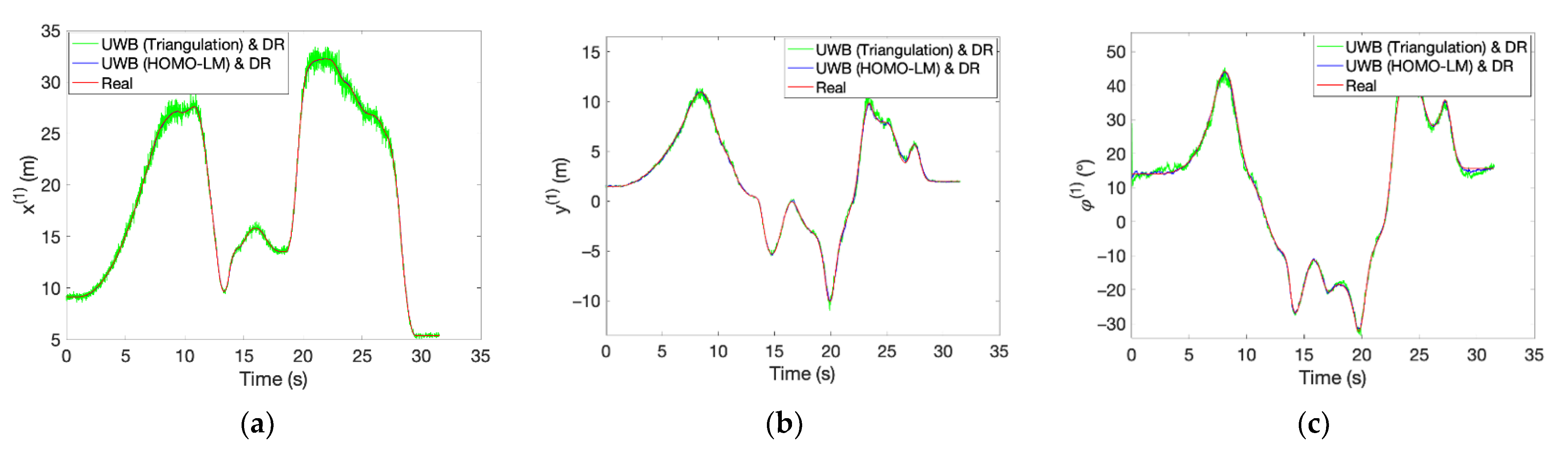
We also conduct a simulation of the UWB/DR fusion system, with results shown in Figure 11. HOMO-LM represents the algorithm with both triangular side length and directed area constraint hereafter.

In comparison to Figure 10, the positioning accuracy is further improved by integrating DR. However, the accuracy improvement was limited after fusion using the traditional triangulation method, especially for longitudinal positioning accuracy. The RPO calculated by the HOMO-LM algorithm lead to apparent better fusion accuracy, especially for longitudinal positioning accuracy.

Table 6. RMSE of position and orientation in simulation.

Algorithm	$\mathit{R}\mathit{M}\mathit{S}{\mathit{E}}_{\mathit{x}} \left(\mathbf{m}\right)$	$\mathit{R}\mathit{M}\mathit{S}{\mathit{E}}_{\mathit{y}} \left(\mathbf{m}\right)$	$\mathit{R}\mathit{M}\mathit{S}{\mathit{E}}_{\mathit{\rho }} \left(\mathbf{m}\right)$	$\mathit{R}\mathit{M}\mathit{S}{\mathit{E}}_{\mathit{\phi }} (°)$
UWB (Triangulation)	0.48	0.50	0.69	32.83
UWB (HOMO-LM)	0.08	0.28	0.29	1.85
UWB (Triangulation) and DR	0.42	0.21	0.47	2.97
UWB (HOMO-LM) and DR	0.02	0.12	0.12	0.38

shows the quantitative comparison results. The root mean square error (RMSE) is recommended to indicate the positioning error. $\rho$ represents the Euclidean distance from the measurement to the real position. $RMS{E}_{\rho }$ represents the absolute positioning error, which is

$$RMS{E}_{\rho }=\sqrt{\frac{{\sum }_{i=1}^n\left[{\left(x_{measure}-x_{real}\right)}^2+{\left(y_{measure}-y_{real}\right)}^2\right]}{n}}$$

(34)

Table 6 shows the same conclusion as Figure 11. The HOMO-LM algorithm provides noticeable better results and contributes to better fusion accuracy as well. The enhanced rate of the RPO accuracy can be computed as

$$\mathit{Enhanced} \mathit{Rate}=\frac{{\mathit{RMSE}}_{\mathit{Classic} \mathit{Algorithm}} - {\mathit{RMSE}}_{\mathit{Prposed} \mathit{Algorithm}}}{{\mathit{RMSE}}_{\mathit{Classic} \mathit{Algorithm}}}$$

(35)

In the pure UWB mode, the proposed HOMO-LM algorithm improved RPO accuracy by 83, 44, 58, and 94%, respectively, in the longitudinal position, lateral position, absolute position, and orientation. In the UWB/DR fusion mode, the proposed algorithm improved the fusion accuracy by 95, 43, 74, and 87%, respectively, in the longitudinal position, lateral position, absolute position, and orientation. The simulation results provided vital support to the proposed algorithm. Therefore, the improvement we made in the localization algorithm was necessary and feasible.

4. Experiments

According to the sources of UWB positioning error we discussed in Section 2, vehicle distance is the only factor that we did not consider in this paper because it is determined by real driving scenarios. Therefore, in this section, the experiments are designed under different vehicle distances. Simulations in Section 3 proved the immense superiority of the proposed HOMO-LM positioning algorithm to the traditional triangulation method. In the experiments, the traditional algorithm was abandoned and would not be verified repeatedly. Nevertheless, the actual timing error cannot be precisely simulated, so the effectiveness of the timing error self-correction method was validated in the experiments.

4.1. Experiment Environment and Equipment

The experimental area and driving routes are shown in Figure 12. Vehicles were driven through a similar route in different experiments but in different vehicle distances.

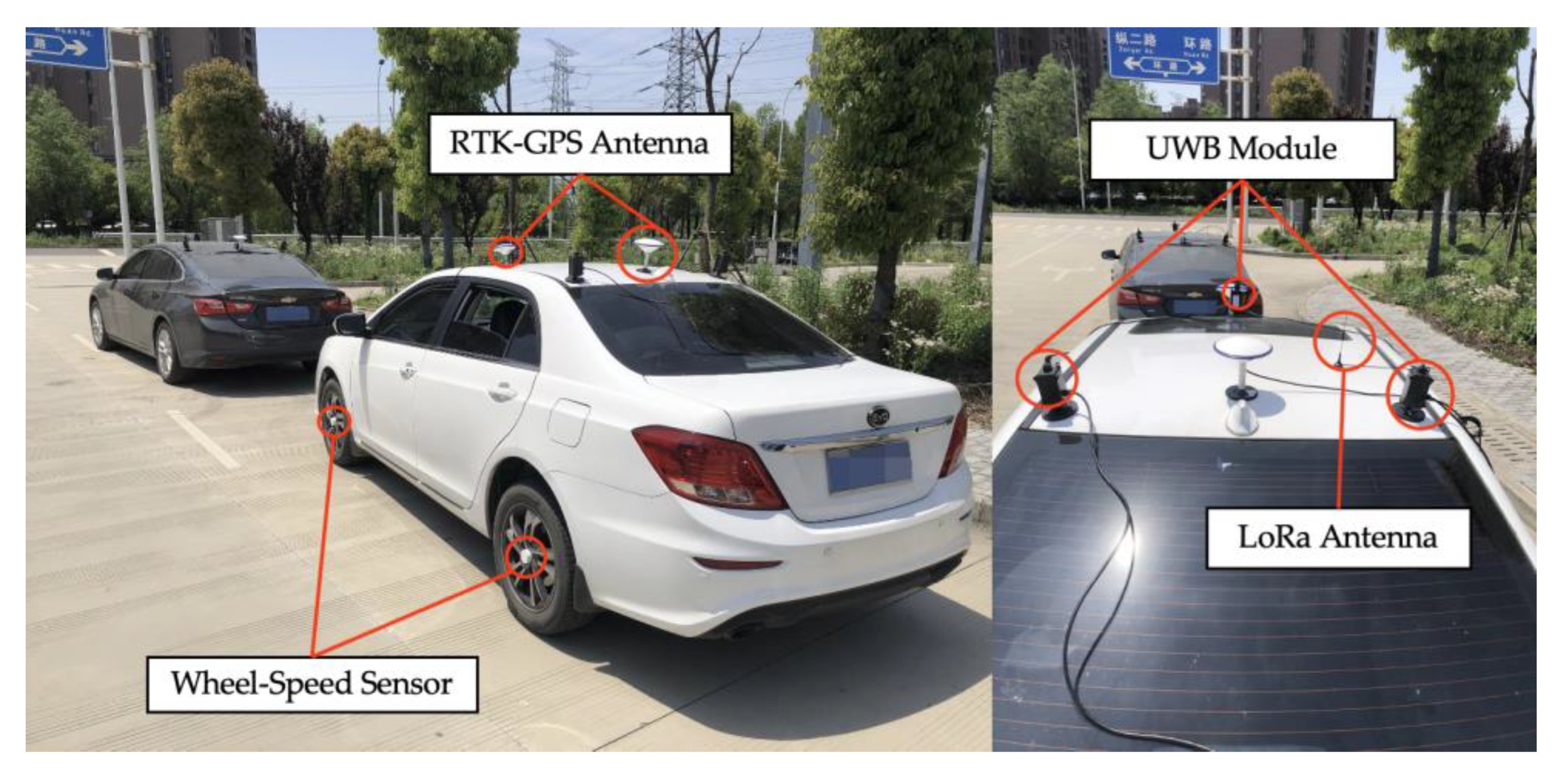
The equipment installed on the vehicles is shown in Figure 13. Two vehicles were necessary, and three UWB modules were installed on top of each vehicle. A high-precision real-time kinematic (RTK)-GPS/INS, which has the positioning accuracy of 1–2 cm, was recognized as the actual reference. Experimental results are compared to the RTK-GPS/INS. A long-range radio (LoRa) antenna was used to receive differential signals from the RTK base station, which was installed in the testing ground.

4.2. Experiment Results

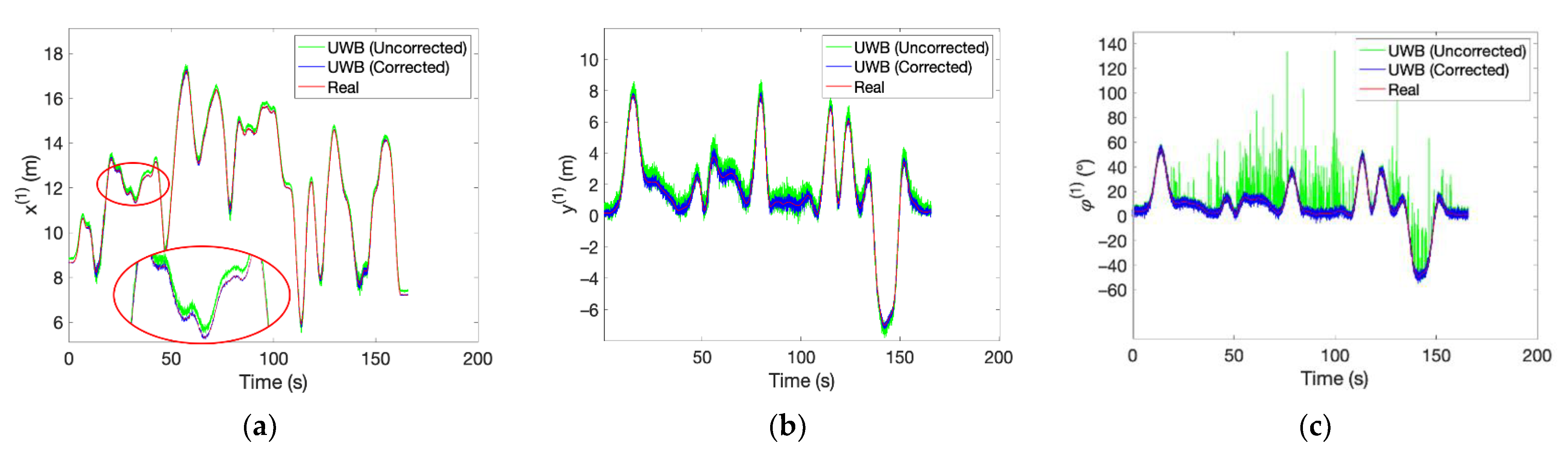
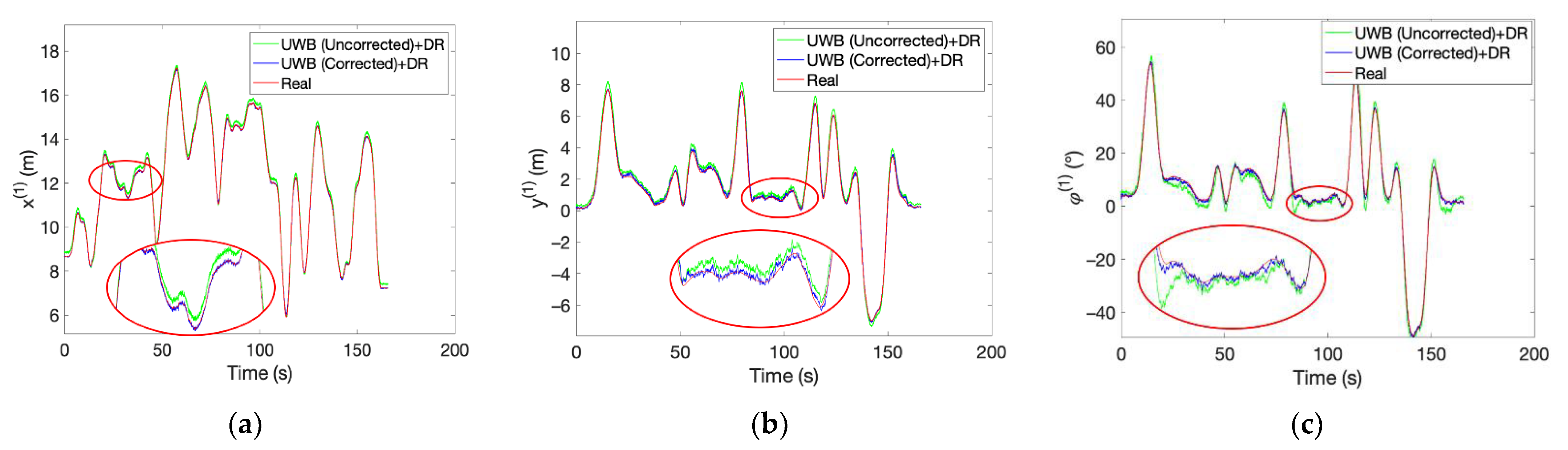
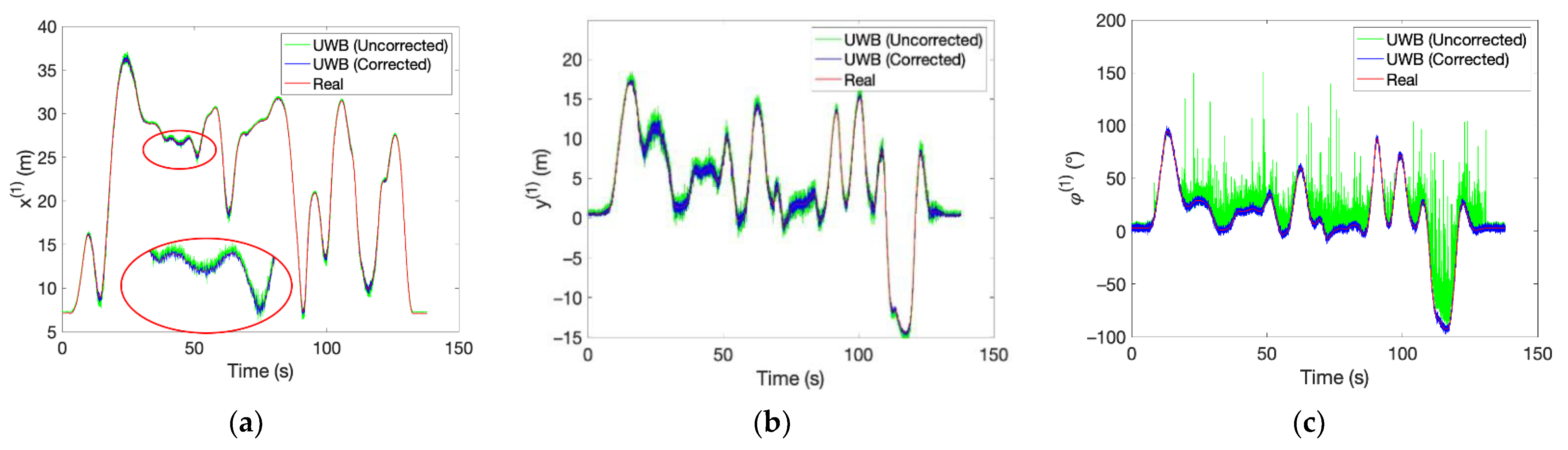
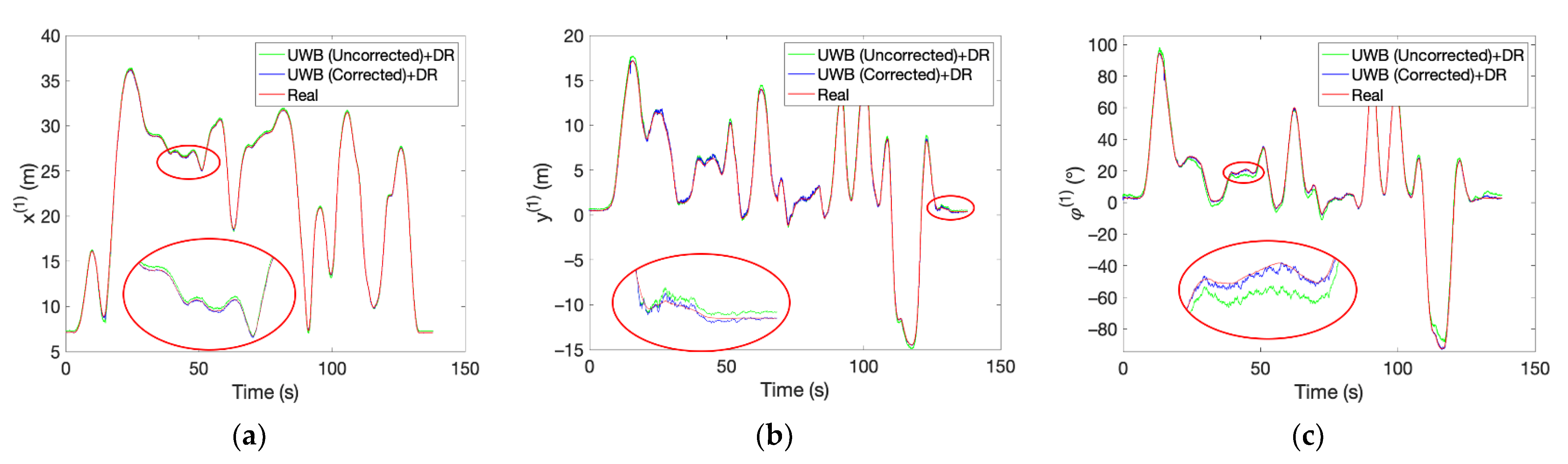
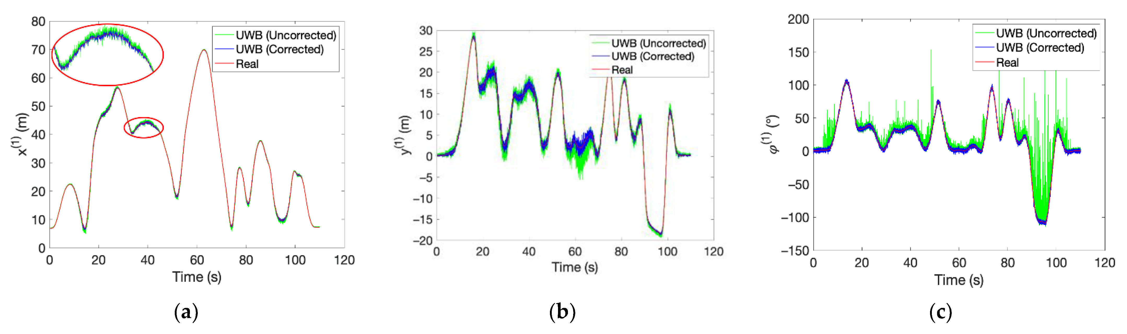
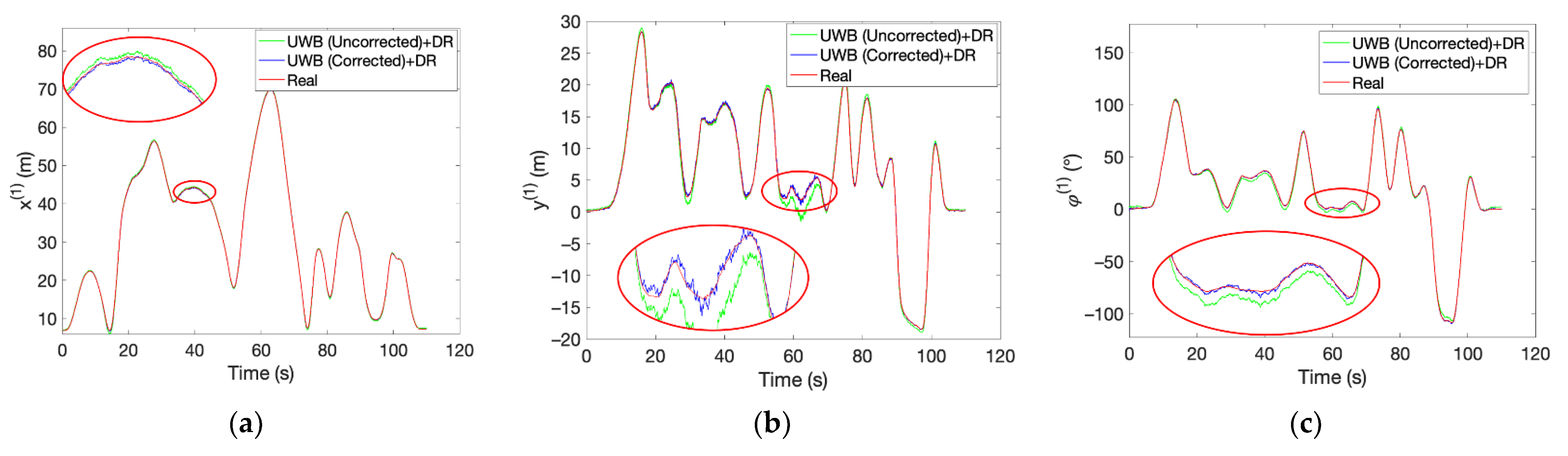
Limited by the size of the testing ground, the two vehicles needed to be closer when turning at corners to keep UWB modules in line of sight. The distance between the two vehicles could not be kept to a constant, so we only guaranteed the maximum vehicle distances during different experiments. The online data of UWB, DR, and RTK-GPS were recorded into the computer and processed in MATLAB/Simulink offline. Figure 14, Figure 15, Figure 16, Figure 17, Figure 18 and Figure 19 show the comparison results of the experiments at maximum vehicle distances of 17 m, 37 m, and 70 m. The quantified positioning deviation from the high precision RTK-GPS/INS is shown in

Table 7. RMSE of the experiment with the maximum distance of 17 m.

Algorithm	$\mathit{R}\mathit{M}\mathit{S}{\mathit{E}}_{\mathit{x}} \left(\mathbf{m}\right)$	$\mathit{R}\mathit{M}\mathit{S}{\mathit{E}}_{\mathit{y}} \left(\mathbf{m}\right)$	$\mathit{R}\mathit{M}\mathit{S}{\mathit{E}}_{\mathit{\rho }} \left(\mathbf{m}\right)$	$\mathit{R}\mathit{M}\mathit{S}{\mathit{E}}_{\mathit{\phi }} (°)$
UWB (Uncorrected)	0.17	0.40	0.43	4.80
UWB(Uncorrected) + DR	0.15	0.30	0.34	2.50
UWB (Corrected)	0.04	0.17	0.17	1.84
UWB (Corrected) + DR	0.04	0.13	0.14	0.66

,

Table 8. RMSE of RPO in the second experiment with the maximum distance of 37 m.

Algorithm	$\mathit{R}\mathit{M}\mathit{S}{\mathit{E}}_{\mathit{x}} \left(\mathbf{m}\right)$	$\mathit{R}\mathit{M}\mathit{S}{\mathit{E}}_{\mathit{y}} \left(\mathbf{m}\right)$	$\mathit{R}\mathit{M}\mathit{S}{\mathit{E}}_{\mathit{\rho }} \left(\mathbf{m}\right)$	$\mathit{R}\mathit{M}\mathit{S}{\mathit{E}}_{\mathit{\phi }} (°)$
UWB (Uncorrected)	0.25	0.63	0.68	11.64
UWB(Uncorrected) + DR	0.18	0.30	0.35	2.36
UWB (Corrected)	0.10	0.32	0.34	1.83
UWB (Corrected) + DR	0.05	0.16	0.17	0.49

and

Table 9. RMSE of RPO in the third experiment with the maximum distance of 70 m.

Algorithm	$\mathit{R}\mathit{M}\mathit{S}{\mathit{E}}_{\mathit{x}} \left(\mathbf{m}\right)$	$\mathit{R}\mathit{M}\mathit{S}{\mathit{E}}_{\mathit{y}} \left(\mathbf{m}\right)$	$\mathit{R}\mathit{M}\mathit{S}{\mathit{E}}_{\mathit{\rho }} \left(\mathbf{m}\right)$	$\mathit{R}\mathit{M}\mathit{S}{\mathit{E}}_{\mathit{\phi }} (°)$
UWB (Uncorrected)	0.38	1.11	1.17	10.26
UWB(Uncorrected) + DR	0.27	0.72	0.77	2.11
UWB (Corrected)	0.16	0.48	0.51	1.83
UWB (Corrected) + DR	0.08	0.22	0.23	0.45

. Similar to simulations, the results of the experiments were also compared in two conditions, the pure UWB mode and UWB/DR fusion mode.

4.3. Results Analysis

Figure 14, Figure 16 and Figure 18 show the comparison results in pure UWB mode. Significant migration exists compared to the real values. As for the orientation, the data was always jumping. For comparison, the results in the UWB/DR fusion mode, shown in Figure 15, Figure 17 and Figure 19, display that the data curves with and without correction are smoother than those in the pure UWB mode, but apparent migration still exists without correction. According to Table 7, Table 8 and Table 9, the effectiveness of the timing error self-correction method is very noticeable. The accuracy of the corrected UWB is even better than that of the uncorrected UWB/DR fusion. In pure UWB mode, the RPO accuracy enhanced rates in the three experiments are computed and shown in

Table 10. RPO accuracy enhanced rate in pure UWB mode in different experiments.

Maximum Vehicle Distance	x	y	$\mathit{\rho }$	φ
17 m	76%	58%	60%	62%
37 m	60%	49%	50%	84%
70 m	58%	57%	56%	82%

, and that in UWB/DR fusion mode is shown

Table 11. RPO accuracy enhanced rate in UWB/DR fusion mode in different experiments.

Maximum Vehicle Distance	x	y	$\mathit{\rho }$	φ
17 m	73%	57%	59%	74%
37 m	72%	47%	51%	79%
70 m	70%	69%	70%	79%

. The RPO accuracy increased substantially either in the pure UWB mode or in the UWB/DR fusion mode. The RPO accuracy improvement with timing error correction was more noticeable in the fusion mode because the UKF eliminates part of the random errors but cannot dispose of system errors, i.e., timing errors, so the influence of timing errors appears more visible.

As shown in Table 7, Table 8 and Table 9, the positioning accuracy decreases with the increase of vehicle distance. However, even in the third experiment with the maximum vehicle distance of 70 m, the calibrated system using the proposed algorithm provided a positioning error of 0.48 m RMSE in the lateral position and 0.2 m RMSE in the longitudinal position. Besides, the relative orientation error was always within 1.85° in all three experiments. It is a significant improvement under the condition that UWB anchors were installed in such a limited space, and the positioning target was so far away. In addition, with the integration of DR, the RPO error decreased to 0.08 m RMSE, 0.22 m RMSE, and 0.45° RMSE, respectively.

5. Conclusions

In this paper, a relative planar localization system with enhanced precision is proposed. We firstly analyze the UWB positioning error sources and confirm that the influencing factors consist of the positioning algorithm, timing errors, and the vehicle distance. Then, a HOMO-LM optimal positioning algorithm is proposed with the triangular side length and directed area constraints, and a UWB timing error calibration method is presented to correct the clock error and antenna delay. Furthermore, a UWB/DR fusion model is established to extend the application scope of the proposed system and evaluate the contribution of the proposed system to integrated positioning accuracy. Finally, simulations and experiments are conducted to validate our work. The main conclusions are as follows:

1

The proposed HOMO-LM method significantly improves the localization precision comparing to the traditional triangulation method. As expected, the side length constraint ensures the positioning accuracy, and the directed area constraint guarantees the stability of the relative orientation. According to the simulation results, in the pure UWB mode, the proposed HOMO-LM algorithm improves RPO accuracy by 87, 44, 58, and 94%, respectively, in the longitudinal position, lateral position, absolute position, and orientation. As for the UWB/DR fusion mode, the proposed algorithm improves the fusion accuracy by 95, 43, 74, and 87%, respectively, in the longitudinal position, lateral position, absolute position, and orientation.

2

The proposed timing error calibration method improves the positioning accuracy significantly. Experimental results show that in the pure UWB mode, the RPO accuracy with timing error correction improves by at least 58, 49, 50, and 62%, respectively, in the longitudinal position, lateral position, absolute position, and orientation. In the UWB/DR fusion mode, the enhanced rate is 70, 47, 50, and 74%, respectively.

3

With the improved algorithm and corrected sensors, even in the third experiment under the maximum vehicle distance at 70 m, our system provided the RPO error within 0.16 m RMSE, 0.48 m RMSE, 0.51 m RMSE, and 1.85° RMSE in the longitudinal position, lateral position, absolute position, and orientation, respectively. Integrated with DR, the RPO error even decreased to 0.08 m RMSE, 0.22 m RMSE, 0.23 m RMSE, and 0.45° RMSE.

References

- Selloum, A.; Betaille, D.; Le Carpentier, E.; Peyret, F. Lane Level Positioning Using Particle Filtering. In Proceedings of the 2009 12th International IEEE Conference on Intelligent Transportation Systems, St. Louis, MO, USA, 4–7 October 2009; pp. 1–6. [Google Scholar]
- Lee, S.; Kim, S.-W.; Seo, S.-W. Accurate Ego-Lane Recognition Utilizing Multiple Road Characteristics in a Bayesian Network Framework. In Proceedings of the 2015 IEEE Intelligent Vehicles Symposium (IV), Seoul, Korea, 28 June–1 July 2015; pp. 543–548. [Google Scholar]
- Casapietra, E.; Weisswange, T.H.; Goerick, C.; Kummert, F.; Fritsch, J. Building a Probabilistic Grid-Based Road Representation from Direct and Indirect Visual Cues. In Proceedings of the 2015 IEEE Intelligent Vehicles Symposium (IV), Seoul, Korea, 28 June–1 July 2015. [Google Scholar] [CrossRef]
- Noureldin, A.; Karamat, T.B.; Georgy, J. Fundamentals of Inertial Navigation, Satellite-Based Positioning and Their Integration; Springer Science & Business Media: Berlin/Heidelberg, Germany, 2012; ISBN 978-3-642-30465-1. [Google Scholar]
- Abdelfatah, W.F.; Georgy, J.; Iqbal, U.; Noureldin, A. 2d Mobile Multi-Sensor Navigation System Realization Using FPGA-Based Embedded Processors. In Proceedings of the 2011 24th Canadian Conference on Electrical and Computer Engineering (CCECE), Niagara Falls, ON, Canada, 8–11 May 2011; pp. 001218–001221. [Google Scholar]
- Berdjag, D.; Pomorski, D. DGPS/INS Data Fusion for Land Navigation. J. Dong Hua Univ. 2004, 21, 88–93. [Google Scholar]
- Barbour, N.; Schmidt, G. Inertial Sensor Technology Trends. IEEE Sens. J. 2001, 1, 332–339. [Google Scholar] [CrossRef]
- Toledo-Moreo, R.; Zamora-izquierdo, M.; Gomez-skarmeta, A. IMM-EKF Based Road Vehicle Navigation with Low Cost GPS/INS. In Proceedings of the 2006 IEEE International Conference on Multisensor Fusion and Integration for Intelligent Systems, Heidelberg, Germany, 3–6 September 2006; pp. 433–438. [Google Scholar]
- Lv, Y.; Liu, Y.; Hua, J. A Study on the Application of WSN Positioning Technology to Unattended Areas. IEEE Access 2019, 7, 38085–38099. [Google Scholar] [CrossRef]
- Katiyar, V.; Kumar, P.; Chand, N. An Intelligent Transportation Systems Architecture Using Wireless Sensor Networks. IJCA 2011, 14, 22–26. [Google Scholar] [CrossRef] [Green Version]
- Li, Q.; Chen, L.; Li, M.; Shaw, S.-L.; Nuchter, A. A Sensor-Fusion Drivable-Region and Lane-Detection System for Autonomous Vehicle Navigation in Challenging Road Scenarios. IEEE Trans. Veh. Technol. 2014, 63, 540–555. [Google Scholar] [CrossRef]
- Zhao, H.; Chiba, M.; Shibasaki, R.; Katabira, K.; Cui, J.; Zha, H. Driving Safety and Traffic Data Collection—A Laser Scanner Based Approach. In Proceedings of the 2008 IEEE Intelligent Vehicles Symposium, Eindhoven, The Netherlands, 4–6 June 2008. [Google Scholar] [CrossRef]
- Sherer, T.P.; Martin, S.M.; Bevly, D.M. Radar Probabilistic Data Association Filter/Dgps Fusion for Target Selection and Relative Range Determination for a Ground Vehicle Convoy. NAVIGATION J. Inst. Navig. 2019, 66, 441–450. [Google Scholar] [CrossRef]
- Patra, S.; Van Hamme, D.; Veelaert, P.; Calafate, C.T.; Cano, J.-C.; Manzoni, P.; Zamora, W. Detecting Vehicles’ Relative Position on Two-Lane Highways through a Smartphone-Based Video Overtaking Aid Application. Mob. Netw. Appl. 2020, 25, 1084–1094. [Google Scholar] [CrossRef]
- Sakjiraphong, S.; Pinho, A.; Dailey, M.N. Real-Time Road Lane Detection with Commodity Hardware. In Proceedings of the 2014 International Electrical Engineering Congress (iEECON), Chonburi, Thailand, 19–21 March 2014; pp. 1–4. [Google Scholar]
- Hang, P.; Lv, C. Human-Like Decision Making for Autonomous Driving: A Noncooperative Game Theoretic Approach. IEEE Trans. Intell. Transp. Syst. 2021, 22, 2076–2087. [Google Scholar] [CrossRef]
- Baek, S.; Kim, H.; Boo, K. Robust Vehicle Detection and Tracking Method for Blind Spot Detection System by Using Vision Sensors. In Proceedings of the 2014 Second World Conference on Complex Systems (WCCS), Agadir, Morocco, 10–12 November 2014; pp. 729–735. [Google Scholar]
- Kim, S.G.; Kim, J.E.; Yi, K.; Jung, K.H. Detection and Tracking of Overtaking Vehicle in Blind Spot Area at Night Time. In Proceedings of the 2017 IEEE International Conference on Consumer Electronics (ICCE), Las Vegas, NV, USA, 8–10 January 2017; pp. 47–48. [Google Scholar]
- Hang, P.; Lv, C.; Huang, C.; Cai, J.; Hu, Z.; Xing, Y. An Integrated Framework of Decision Making and Motion Planning for Autonomous Vehicles Considering Social Behaviors. IEEE Trans. Veh. Technol. 2020, 69, 14458–14469. [Google Scholar] [CrossRef]
- Ma, H.; Ma, Y.; Jiao, J.; Bhutta, M.U.M.; Bocus, M.J.; Wang, L.; Liu, M.; Fan, R. Multiple Lane Detection Algorithm Based on Optimised Dense Disparity Map Estimation. In Proceedings of the 2018 IEEE International Conference on Imaging Systems and Techniques (IST), Krakow, Poland, 16–18 October 2018; pp. 1–5. [Google Scholar]
- Amimi, O.; Mansouri, A.; Dose Bennani, S.; Ruichek, Y. Stereo Vision Based Advanced Driver Assistance System. In Proceedings of the 2017 International Conference on Wireless Technologies, Embedded and Intelligent Systems (WITS), Fez, Morocco, 19–20 April 2017; pp. 1–5. [Google Scholar]
- Peng, Z.; Hussain, S.; Hayee, M.I.; Donath, M. Acquisition of Relative Trajectories of Surrounding Vehicles Using GPS and SRC Based V2V Communication with Lane Level Resolution. In Proceedings of the 3rd International Conference on Vehicle Technology and Intelligent Transport Systems; SCITEPRESS—Science and Technology Publications: Porto, Portugal, 2017; pp. 242–251. [Google Scholar]
- Shen, F.; Cheong, J.W.; Dempster, A.G. A DSRC Doppler/IMU/GNSS Tightly-Coupled Cooperative Positioning Method for Relative Positioning in VANETs. J. Navig. 2017, 70, 120–136. [Google Scholar] [CrossRef] [Green Version]
- de Ponte Muller, F.; Diaz, E.M.; Rashdan, I. Cooperative Positioning and Radar Sensor Fusion for Relative Localization of Vehicles. In Proceedings of the 2016 IEEE Intelligent Vehicles Symposium (IV), Gothenburg, Sweden, 19–22 June 2016; pp. 1060–1065. [Google Scholar]
- Pinto Neto, J.B.; Gomes, L.C.; Ortiz, F.M.; Almeida, T.T.; Campista, M.E.M.; Costa, L.H.M.K.; Mitton, N. An Accurate Cooperative Positioning System for Vehicular Safety Applications. Comput. Electr. Eng. 2020, 83, 106591. [Google Scholar] [CrossRef] [Green Version]
- Sakkila, L.; Tatkeu, C.; Boukour, F.; El Hillali, Y.; Rivenq, A.; Rouvean, J.-M. UWB Radar System for Road Anti-Collision Application. In Proceedings of the 2008 3rd International Conference on Information and Communication Technologies: From Theory to Applications, Damascus, Syria, 7–11 April 2008; pp. 1–6. [Google Scholar]
- Shi, D.; Mi, H.; Collins, E.G.; Wu, J. An Indoor Low-Cost and High-Accuracy Localization Approach for AGVs. IEEE Access 2020, 8, 50085–50090. [Google Scholar] [CrossRef]
- Xue, W.-W.; Jiang, P. The Research on Navigation Technology of Dead Reckoning Based on UWB Localization. In Proceedings of the 2018 Eighth International Conference on Instrumentation & Measurement, Computer, Communication and Control (IMCCC), Harbin, China, 19–21 July 2018; pp. 339–343. [Google Scholar]
- Monica, S.; Ferrari, G. Low-Complexity UWB-Based Collision Avoidance System for Automated Guided Vehicles. ICT Express 2016, 2, 53–56. [Google Scholar] [CrossRef] [Green Version]
- Pittokopiti, M.; Grammenos, R. Infrastructureless UWB Based Collision Avoidance System for the Safety of Construction Workers. In Proceedings of the 2019 26th International Conference on Telecommunications (ICT), Hanoi, Vietnam, 8–10 April 2019; pp. 490–495. [Google Scholar]
- Zhang, R.; Song, L.; Jaiprakash, A.; Talty, T.; Alanazi, A.; Alghafis, A.; Biyabani, A.A.; Tonguz, O. Using Ultra-Wideband Technology in Vehicles for Infrastructure-Free Localization. In Proceedings of the 2019 IEEE 5th World Forum on Internet of Things (WF-IoT), Limerick, Ireland, 15–18 April 2019; pp. 122–127. [Google Scholar]
- Theussl, E.-J.; Ninevski, D.; O’Leary, P. Measurement of Relative Position and Orientation Using UWB. In Proceedings of the 2019 IEEE International Instrumentation and Measurement Technology Conference (I2MTC), Auckland, New Zealand, 20–23 May 2019; pp. 1–6. [Google Scholar]
- Ghanem, E.; O’Keefe, K.; Klukas, R. Testing Vehicle-to-Vehicle Relative Position and Attitude Estimation Using Multiple UWB Ranging. In Proceedings of the 2020 IEEE 92nd Vehicular Technology Conference (VTC2020-Fall), Victoria, BC, Canada, 18 November–16 December 2020; pp. 1–5. [Google Scholar]
- Akopian, D.; Melkonyan, A.; Chen, C.L.P. Validation of HDOP Measure for Impact Detection in Sensor Network-Based Structural Health Monitoring. IEEE Sens. J. 2009, 9, 1098–1102. [Google Scholar] [CrossRef]
- Bonnin-Pascual, F.; Ortiz, A. UWB-Based Self-Localization Strategies: A Novel ICP-Based Method and a Comparative Assessment for Noisy-Ranges-Prone Environments. Sensors 2020, 20, 5613. [Google Scholar] [CrossRef] [PubMed]
- Zhang, L.; Zhou, W.; Li, D. Global Convergence of a Modified Fletcher–Reeves Conjugate Gradient Method with Armijo-Type Line Search. Numer. Math. 2006, 104, 561–572. [Google Scholar] [CrossRef]
- Sorkine-Hornung, O.; Rabinovich, M. Least-Squares Rigid Motion Using SVD. Computing 2017, 1, 1–5. [Google Scholar]
- Julier, S. A General Method for Approximating Nonlinear Transformations of Probability Distributions. Citeseer 1996. [Google Scholar] [CrossRef] [Green Version]
- Wan, E.A.; Van Der Merwe, R.; Nelson, A.T. Nelson Dual Estimation and the Unscented Transformation. NIPS 1999, 29, 666–672. [Google Scholar]
Figure 1.
Sources of UWB Positioning error. Red boxes show the factors that we will address in the proposed system. The blue box shows the variable that we will control in the experiments.
Figure 2.
The relative positioning and directing model.
Figure 3.
The real triangle and the calculated triangles using different methods: (a) the classic triangulation method; (b) the LS method with side length constraint; (c) the LS method with side length and directed area constraint.
Figure 4.
Two-way ranging model. Module i sends a signal to module j firstly. Then module j receives the signal and sends a signal back to module i immediately. In the ranging process, the sending and receiving delays and the clock errors of the two modules will affect the ranging accuracy.
Figure 5.
The circulation calibration mode: (a) Module A firstly send a signal, and BC send signals in turn after receiving signals from the former module; (b) Module B firstly sends a signal and CA sends signals in turn after receiving signals from the former module; (c) Module A firstly send a signal, and BC send signals in turn after receiving signals from the former module.
Figure 6.
The differential calibration mode: (a) signals transmit from A to C in two paths; (b) signals transmit from B to A in two paths; (c) signals transmit from C to B in two paths.
Figure 7.
The DR model based on four wheel-speed sensors and IMU.
Figure 8.
The relative kinematic model.
Figure 9.
The virtual scenario in the Driving Scenario Designer. The blue cube represents vehicle 1. The red cube represents vehicle 2. The blue/red dots indicate the waypoints of the two vehicles defined in the Driving Scenario Designer.
Figure 10.
Simulation results for the proposed HOMO-LM method: (a) the relative longitudinal position; (b) the relative lateral position; (c) the relative orientation.
Figure 11.
Simulation results of UWB and DR fusion: (a) Relative longitude position; (b) Relative lateral position; (c) Relative orientation.
Figure 12.
The routes of two vehicles in the experiments.
Figure 13.
Experimental equipment.
Figure 14.
Comparison of UWB localization data with and without correction in the experiment with maximum vehicle distance of 17 m: (a) the relative longitudinal position; (b) the relative lateral position; (c) the relative orientation.
Figure 15.
Comparison of fusion localization with and without correction in the experiment with maximum vehicle distance of 17 m: (a) the relative longitudinal position; (b) the relative lateral position; (c) The relative orientation.
Figure 16.
Comparison of UWB localization data with and without correction in the experiment with maximum vehicle distance of 37 m: (a) the relative longitudinal position; (b) the relative lateral position; (c) the relative orientation.
Figure 17.
Comparison of fusion localization with and without correction in the experiment with maximum vehicle distance of 37 m: (a) the relative longitudinal position; (b) the relative lateral position; (c) the relative orientation.
Figure 18.
Comparison of UWB localization data with and without correction in the experiment with maximum vehicle distance of 70 m: (a) the relative longitudinal position; (b) the relative lateral position; (c) the relative orientation.
Figure 19.
Comparison of fusion localization with and without correction in the experiment with maximum vehicle distance of 70 m: (a) the relative longitudinal position; (b) the relative lateral position; (c) the relative orientation.