
Robust Model Reference Adaptive Control for Tail-Sitter VTOL Aircraft


1
Middle Technical University/Electrical Engineering Technical College, Baghdad 10001, Iraq
2
Control and Systems Engineering Department, University of Technology, Baghdad 10001, Iraq
3
Department of Electrical Engineering, College of Engineering, University of Baghdad, Baghdad 10001, Iraq
4
College of Computer and Information Sciences, Prince Sultan University, Riyadh 11586, Saudi Arabia
5
Faculty of Computers and Artificial Intelligence, Benha University, Benha 13511, Egypt
*
Author to whom correspondence should be addressed.
Actuators 2021, 10(7), 162; https://0-doi-org.brum.beds.ac.uk/10.3390/act10070162
Submission received: 25 May 2021
/
Revised: 24 June 2021
/
Accepted: 25 June 2021
/
Published: 15 July 2021
(This article belongs to the Section Control Systems)
Abstract
:This study presents a control design of roll motion for a vertical take-off and landing unmanned air vehicle (VTOL-UAV) design based on the Model Reference Adaptive Control (MRAC) scheme in the hovering flight phase. The adaptive laws are developed for the UAV system under nonparametric uncertainty (gust and wind disturbance). Lyapunov-based stability analysis of the adaptive controlled UAV system under roll motion has been conducted and the adaptive laws have been accordingly developed. The Uniform Ultimate Boundness (UUB) of tracking error has been proven and the stability analysis showed that the incorporation of dead-zone modification in adaptive laws could guarantee the uniform boundness of all signals. The computer simulation has been conducted based on a proposed controller for tracking control of the roll motion. The results show that the drift, which appears in estimated gain behaviors due to the application of gust and wind disturbance, could be stopped by introducing dead-zone modification in adaptive laws, which leads to better robustness characteristics of the adaptive controller.
1. Introduction
In the last several decades, Unmanned Aerial Vehicles (UAVs) have gained fast-growing popularity world-wide and experienced enormous development. Nowadays, the UAVs are extensively applied in various critical defense and military purposes such as reconnaissance, security reinforcement and surveillance. However, in addition to military and defense applications of UAVs, the usage of these small aircraft has rapidly grown in many civilian applications and covered a wide range of areas including disaster management, traffic surveillance, vegetarian monitoring infrastructure inspection, and law enforcement [1].
There are other missions of UAV which extend the scope of conventional capabilities of small UAVs. The longer endurance of flight is not only the requirement of most missions, but also the vertical takeoff and landing (VTOL) and hovering capabilities. Moreover, the capability of conversion from one configuration to another is the other required task of these small aircrafts, which became necessary recently. Combing the forward flight characteristics of fixed-wing aircraft with the takeoff and landing capabilities of the helicopter will result in promising UAVs which are characterized by unique flexible operation capabilities at low cost compared to other conventional UAVs [2].
The Tail-sitter vehicle is one configuration of these convertible aircrafts. It is characterized by taking the vertical airframe attitude during landing and takeoff, while taking the attitude of the horizontal airframe in the case of cruising, just like conventional airplanes. However, the flight dynamics of Tail-sitters are characterized by high complexity, particularly in hover mode, which makes them very difficult to control [2]. In what follows, some of the relevant and recent control strategies used for flight control of Tail-sitter aircraft are briefly discussed.
Jacson MO Barth proposed a flight control design based on a model-free control strategy to stabilize the attitude of tail-sitter micro-aircraft (Darko type) subjected to wind disturbance in four flight modes—vertical takeoff, transitioning flight, forward flight, hovering and vertical landing. The proposed controller has been tested and compared to another incremental nonlinear dynamic inversion controller based on computer simulation and real experiment [3].
Zhou et al. (2019) presented the design of a model predictive controller for a VTOL tail-sitter UAV based on a successive linearization in the hovering flight with vertical take-off and landing phases. The controller has been established based on state–space prediction model, which is augmented with feedback integration terms and estimated disturbance. The controlled system has been firstly tested based on software-in-loop simulation and then verified via real-time indoor flight tests. It has been shown that the controller could give precise trajectory tracking with good stability characteristics in the presence of wind disturbance [4].
Wang et al. (2019) proposed a novel configuration design for the twin rotor tail-sitter. The presented configuration could achieve high disturbance rejection capability by decreasing the distance between elevators and rotors. This leads to maximizing the speed of airflow such as to generate the adequate control torque necessary to stabilize the UAV against wind disturbance [5].
Nieto et al. (2019) presented the design and implementation of the control system to perform a VTOL maneuver for unmanned Flying-wing using two tilting rotors (Bi-Rotor). The work has developed the nonlinear dynamics of Bi-rotor UAV and designed the attitude tracking controller in hovering operation. The Hardware-In-the-Loop (HIL) simulation and experimental tests have been applied to verify the controller’s efficiency [6].
Ge and Hou (2019) combined the design of L1 adaptive control and fuzzy self-tuning PID control for stabilizing the longitudinal attitude of the Tail-Sitter UAV with the presence of disturbance. In this study, the singularity problem of pitch angle, which appears during fuselage tilting, has been solved by applying the double Euler angle algorithm in modeling. The computer simulation showed the control design could compensate the effect due to parametric and nonparametric uncertainty (disturbance) [7].
Abrougui et al. (2019) developed a flight regulation algorithm based on Proportional-Integral and Derivative (PID) control for roll motion stabilization of VTOL-UAV during hovering flight. The effectiveness of the conventional controller has been verified using computer simulation. The controller has been tested experimentally based on the AtMega2560 micro-controller [8].
Flores (2018) presented a control design for maneuver transition of a tail-sitter drone based on the Lyapunov approach and linear saturation functions. The proposed controller focused on time-scale separation between drone attitude and position. Simulated and experimental results have been used to verify the effectiveness of the proposed controller [9].
Garcia et al. (2008) applied the separated saturation functions to develop a control algorithm for stabilizing a single-rotor tail UAV subjected to perturbation in vertical take-off landing. The dynamic model of the aircraft is firstly developed and the performance of the controller has been evaluated based on computer simulation and real-time tests in autonomous hover flights of aircrafts [10].
Verling et al. (2016) presented the design and control of convertible VTOL tail-sitter UAVs. The developed UAV has mixed advantages of both fixed and rotary wing technologies of UAV systems. A novel controller, which is functioning in SO (3), has been developed to cope with the vehicle dynamics at any attitude configuration, like the rotorcraft and fixed-wing scheme as well as the transitions from one configuration to another. The proposed unified controller can permit smooth transition without discontinuations in switching. The effectiveness of the platform and controller was evaluated using extensive experimental tests [11].
Li et al. (2016) presented the design of an MPC (Model Predictive Controller) to control the position of Tail-Sitter VTOL aircraft during flight in hovering mode. The model predictive control algorithm has been developed based on an augmented linearized model. An optimization technique has been applied to enhance disturbance rejection capability. The HIL (Hardware-in-loop) simulation is used to assess the performance of the proposed controller, which also has been tested experimentally within an indoor space based on the on-board flight computer. The simulated and experimental results showed good robustness of MPC against gusty wind [12].
Çakici and Kemal (2016) presented the design of the control system for the UAV based on three modes—VTOL, hover and level flight capability. The considered structure of aircraft includes fixed wings (FW) and multi-rotors. The proposed design included the development of a control algorithm to switch between two modes. The effectiveness of the controller has been examined experimentally [13].
Like most aircrafts, the dynamics of Tail-sitters encounter dramatic variations during their flight and the need for a robust controller is a pre-requisite to solve this challenging problem. However, the use of a conventional controller is awesome for these kinds of aerial systems. One of the drawbacks of conventional tracking controllers is that they are unable to cope with unknown load characteristics over a wide range of operating points. Apparently, this makes tuning of controller parameters very difficult. There are many ways to overcome these difficulties, but, generally, there are four basic ways that are common to the adaptive controller—Model reference adaptive control (MRAC), Gain scheduling, Dual control and Self tuning [14]. In the presence of parametric and/or nonparametric uncertainties, it has been shown that the MRAC is the proper control technique to cope with such uncertainties and to achieve proper precision of tracking control [15].
In the adaptive control technique, the parameters of a plant in real-time are adjusted in order to keep a desired level of dynamic performance when the system is subjected to unknown and varying (changing with time) parameters [16,17,18,19]. In the real world, the MRAC offers an approach to solve the problems concerning the adaptive control by synthesizing a closed-loop controller, where the MRAC compares the standard reference with the plant response such that the various parameters will be changed accordingly [17].
One critical problem in the adaptive model reference control is that the developed adaptive laws may not guarantee bounded estimated gains in the presence of unknown uncertainties. In the case that all uncertainties can be structurally known and linearly parameterized, then these uncertainties can be exactly compensated and the global stability of adaptive-controlled systems can be guaranteed [20,21,22]. However, these assumptions are not feasible in most real physical systems, since the presence of nonparametric uncertainties such as sensor noise, delays, unmodeled dynamics (e.g., actuators, structural dynamics), time-varying disturbances (e.g., wind gust), and numerical and quantization errors are always inevitable. As such, the controlled system based on MRAC may suffer from degradation in robustness characteristics with the presence of these nonparametric uncertainties. The reason behind this can be argued in the sense of Lyapunov-based stability analysis, where the time derivative of the Lyapunov function becomes a sign-indefinite function in the presence of nonparametric and unmatched uncertainties [23,24,25].
To guarantee the boundedness of the adaptive parameters, different robustness modification techniques have been proposed in the literature, where the most important ones are σ-modification, e-modification, Dead Zone, Parameter Projection, and Optimal-modification [26,27,28,29]. In this work, the e-modification has been proposed for its simplicity and effectiveness. Therefore, the drifting of estimated gains in using adaptive model reference control of UAVs is the critical problem to be addressed and solved by the present work and the contribution of the work can be highlighted by these main points:
- □
- Design of Model Reference Adaptive Controller for tracking control of roll attitude for the Tail-Sitter VTOL aircraft;
- □
- Development of adaptive laws that guarantee bounded convergence of tracking and estimation error of controlled aircraft based on Lyapunov stability analysis; and
- □
- Improvement of the robustness characteristics for Model Reference Adaptive Controlled aircraft by modifying the developed adaptive laws using dead-zone modification.
2. Dynamic Model of Tail-Sitter VTOL UAV
This section considers the development of a dynamic model for the Tail-Sitter VTOL Aircraft. Firstly, two assumptions are made to proceed in deriving the dynamic model:
Assumption 1: The aircraft operates within small local region. This will justify to apply the model equation of Flat-Earth [13]; and
Assumption 2: The masses of blade and elevators have been neglected [30].
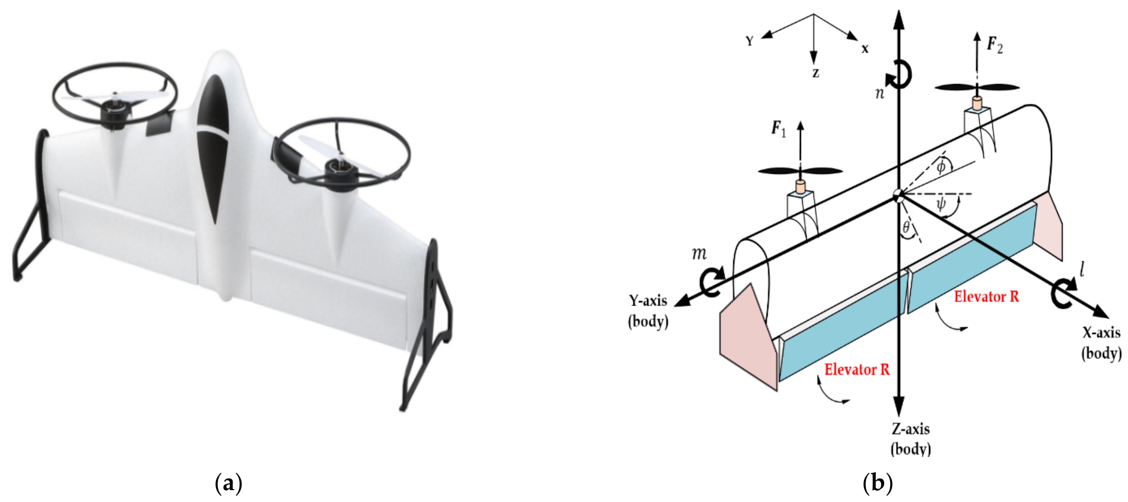
Referring to Figure 1, let the coordinate system () represent the body fixed frame and the north-east-down (NED) coordinate system () represent the inertial reference frame (). Based on Figure 1, the kinematic equations describing the position, the forces and the moments are represented by [31]:
where represents the transformation matrix from airframe to the fixed inertial coordinate and it is given by
where represents and represents . represents the positions of mass of the center of the rigid body relative to the (), represents the quaternion of the current attitude and it is defined by , which represents the orientation of the VTOL aircraft in the (). represents the transformation matrix of the angular velocity generated by a sequence of Euler rotations from the body to the local reference system during hover flight and it is defined by:
where 𝑡𝑎 denotes tan(a) and the Euler angles , and define the roll, pitch and yaw angles, which are commonly used in aerodynamic applications. The vector represents the angular velocity in the body fixed frame , is the vector of external thrusts applied to mass center of the VTOL aircraft, the torque vector combines the torque components applied to the mass center of VTOL aircraft in the body frame and is the inertia matrix of the flying aircraft, which is given by
If it is assumed the body axis -plane of the configuration of tail-sitter VTOL aircraft is coincident with the plane of symmetry, then the products of inertia and vanish. Also, the tail-sitter configuration has a plane of symmetry in the -plane, and this leads to the product of inertia being equal to zero. Then, the inertia matrix and its inverse becomes
The transformation matrix given in Equation (2) transforms the components of the angular velocity, generated by Euler rotations, from the body frame to the inertial frame, which is given by:
Therefore, the kinematic Equation (2) can be written as follows:
Using the inertia matrix given by Equation (6) and using the thrust moments , and as indicated in Figure 1, Equation (4) can be rewritten by:
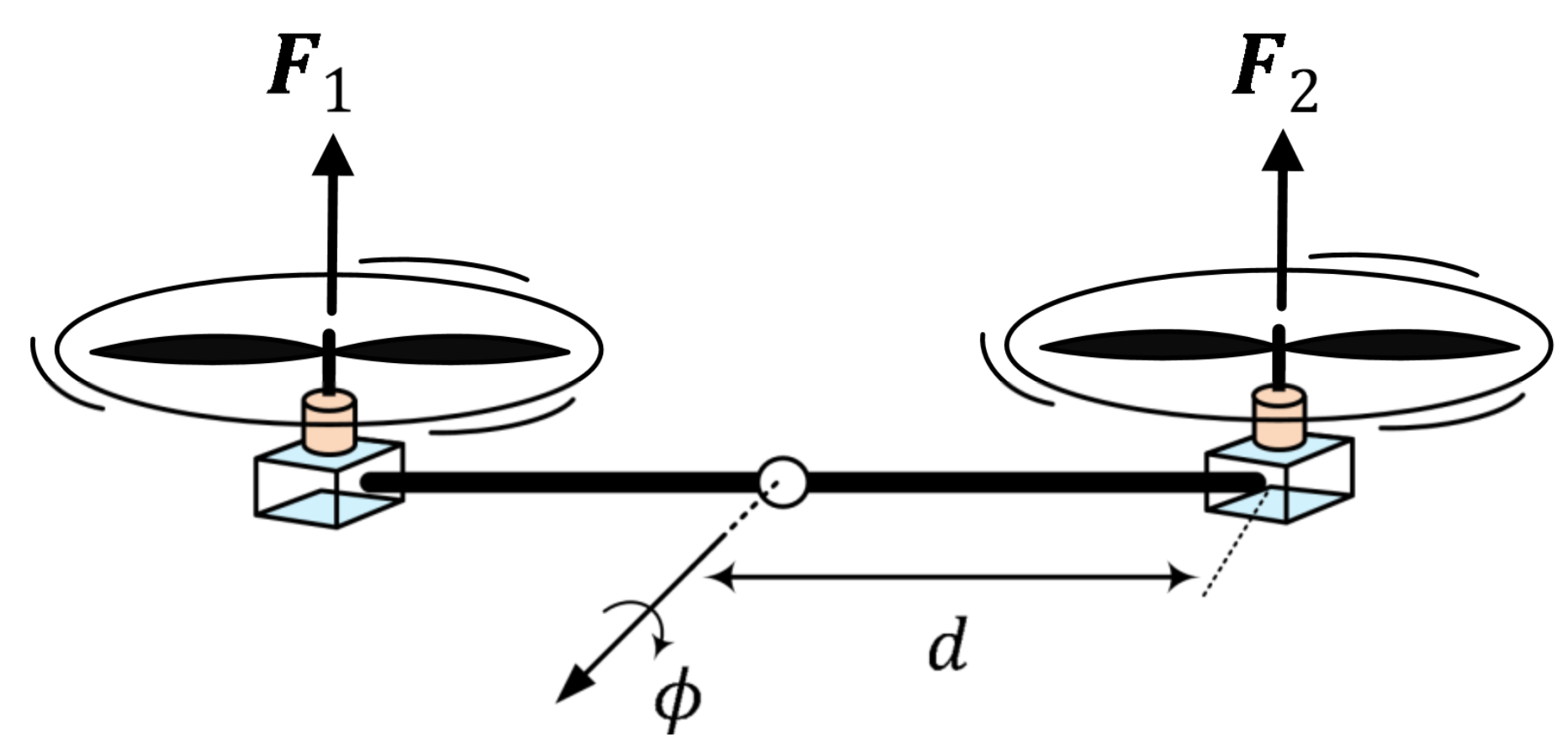
In order to extract the roll dynamic, it is assumed that the yaw and pitch rates are set to zero; that is, . Based on this assumption, the configuration of tail-sitter VTOL aircraft is shown in Figure 2. Therefore, based on Equations (6) and (9), the rotational dynamics can be represented for the roll angle using the following simple dynamic equation:
where the exerted torque can be calculated as follows:
where represents the resultant force between the force due to right rotor and left rotor, is the distance between the mass center and reach rotor. The term is the drag force, which represents the aerodynamic moment that works to oppose the rolling moment with a damping coefficient of .
Combining Equations (14) and (15) and taking into account the effect of gust wind as uncertainty applied to the roll dynamic system, we have
In order to establish the state space of Equation (13), one can let , and to have the following state variable:
3. Design of Adaptive Model Reference Control for Tail-Sitter VTOL Aircraft
Comparing Equation (17) to the above equation, one can have
Let us consider the stable model reference model given by the general second order transfer function:
where and represent the natural un-damped frequency and damping ratio, respectively. In matrix form, Equation (20) becomes
or,
The structure of the ideal control law is proposed to consist of state feedback and feed forward parts as follows:
where and are the ideal feedback and feed-forward gain matrices, respectively. Substituting Equation (23) into Equation (18), one can obtain,
In order for the actual state to coincide with the model reference, the matching condition has to be satisfied
Using Equations (19), (21) and (25), one can get
Equation (26) proves that the matching condition is satisfied.
Based on Equation (23), the estimated control law will have the following structure
where and are the estimates of the ideal gains and , repectively.
Substituting the actual control law of Equation (27) into Equation (18), one can have
If the state tracking error is defined by
In order to achieve a perfect tracking of errors, all signals in the closed-loop system have to remain uniformly bounded. Thus, given any bounded command , the control input needs to be chosen such that the state tracking error tends to zero in a globally, uniformly and asymptotically manner, that is,
Taking the time derivative of state error
Substituting Equations (22) and (28) into Equation (31), one can have
Using the matching conditions of Equation (25), one can get
where , are the estimation errors in feedback and feed-forward gain vectors, repectively.
Let us consider a bounded and quadratic Lyapunov candidate function:
where , are the matrices of adaptation rate. The matrix will be later determined.
Taking the time derivative of the Lyapunov function and assuming stationary values of ideal gains (, one can have
or,
Using the algebraic fact , the following terms can be written in terms of trace function,
Using Equations (36)–(38), we derive
where is used to guarantee the negative definite of the first term of Equation (39) by solving the matrix based on the following expression:
According to Equation (39), the adaptive laws can be deduced
Theorem 1.
For the system describe by Equation (18), which is subjected to uncertainties, the adaptive control can be developed based on control law defined by Equation (23) to yield adaptive laws, described by Equations (41) and (42), which result in bounded tracking error.
Proof.
Based on adaptive laws, the -equation reduces to
Form linear algebra, using the Rayleigh–Ritz method [32], Equation (43) results in
or,
where and are the minimum and maximum eigenvalues of matrix and , respectively. According to Equation (45), outside the set
Based on Equation (46), one can conclude that the trajectories of tracking error will come into the set in finite time and stay thereafter. □
However, the set is not compact in the space. Also, the set is unbounded since the gain estimation errors () are not restricted. Therefore, the Lyapunov function may become positive inside , thereby can grow unbounded, in spite of the fact that the tracking error norm remains finite for all times. This drift in arises due to the disturbance term , which was small.
4. Robust Adaptive Model Reference Control
In order to prevent the drift in adaptive gains and , modifications of adaptive laws, are introduced. In the present work, the dead-zone modification has been proposed to improve the robustness of the adaptive model reference controller as follows:
Therefore, when the error enters the set , the adaptation process is frozen and and will be bounded. Hence, the ultimate upper bound (UUB) of tracking error and the estimation error are guaranteed.
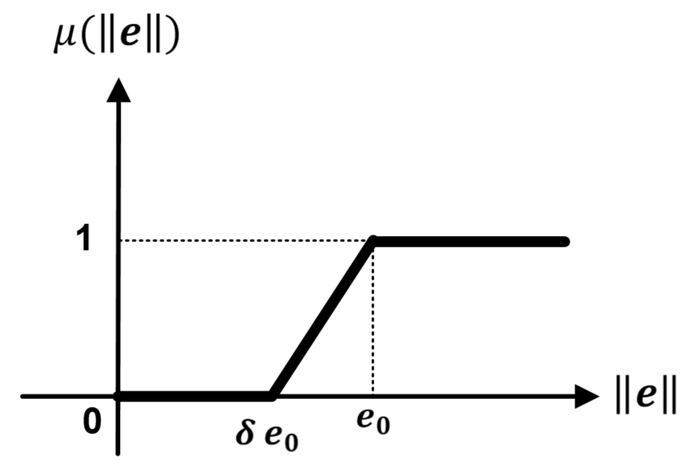
However, the dead-zone modification described by Equations (47) and (48) is not Lipschitz. Therefore, it may lead to chattering or undesirable effects, especially when the error is adjacent to the boundary of dead-zone. The dead-zone modification can be replaced by a Lipschitz-continuous modulation function described by Figure 3 and defined by [33]:
Based on the continuous dead-zone modification, the adaptive laws can be defined by
Theorem 2.
The adaptive laws based on dead-zone technique and given by Equations (50) and (51) lead to UUB of all signals, which results in robust adaptive control that prevents the drift in adaptive parameters.
Proof.
As indicated from Equations (46) and (47), the adaptation process is enabled when , while the adaptation process is frozen when such that the potential parameter drift is avoided as . One can choose the following Lyapunov candidate function:
The tracking error can be expressed as
Therefore, the time derivative of Lyapunov function is given by
or,
Since is required, then the following inequality has to be satisfied
Using from linear algebra, one can have
Since , is also bounded. Thus, the adaptive law based on dead-zone technique is robust and the parameter drift is prohibited. □
Figure 4 shows the schematic diagram of robust model reference adaptive control for Tail-Sitter VTOL aircraft.
5. Computer Simulation
In this section, the effectiveness of the proposed controller has been verified based on simulated results within MATLAB programming format (R 2016b). The s-functions are used to develop the codes of VYOL aircraft dynamics, control law and adaptive laws. The Ode45 has been selected as a numerical solver in the computer simulation and the variable-hit option has been chosen for the solver, where both maximum and minimum step size are set to auto-option. Table 1 gives the numerical values of parameters for considering Tail-Sitter VTOL Aircraft.
Three scenarios have been presented—the first scenario considered the uncertainty-free case, the second scenario has taken into account the presence of uncertainty, which represents the wind gust, while the third scenario addressed the drift problem in adaptive law.
Firstly, the following calculation has to be performed a priori. Based on Table 1, the numeric structure of the system model is given by
The controllability matrix has to be established and checked in control design; that is, the pair must be controllable:
It is evident that the controllability matrix has rank = 2 and the system is completely controllable. The natural damping coefficient and the natural un-damped frequency of the model reference are and . The values of adaptive rate matrices are set by:
The matrix can be calculated according to , where is set to be the identity matrix (positive definite),
This indicates that is a positive definite matrix.
The next step is to find the values of gain matrices and using matching condition of Equation (25). Based on Equation (26), , one can obatin , . Using the second part of matching condition , one can easily get .
5.1. Scenario I: Uncertainty-Free Case
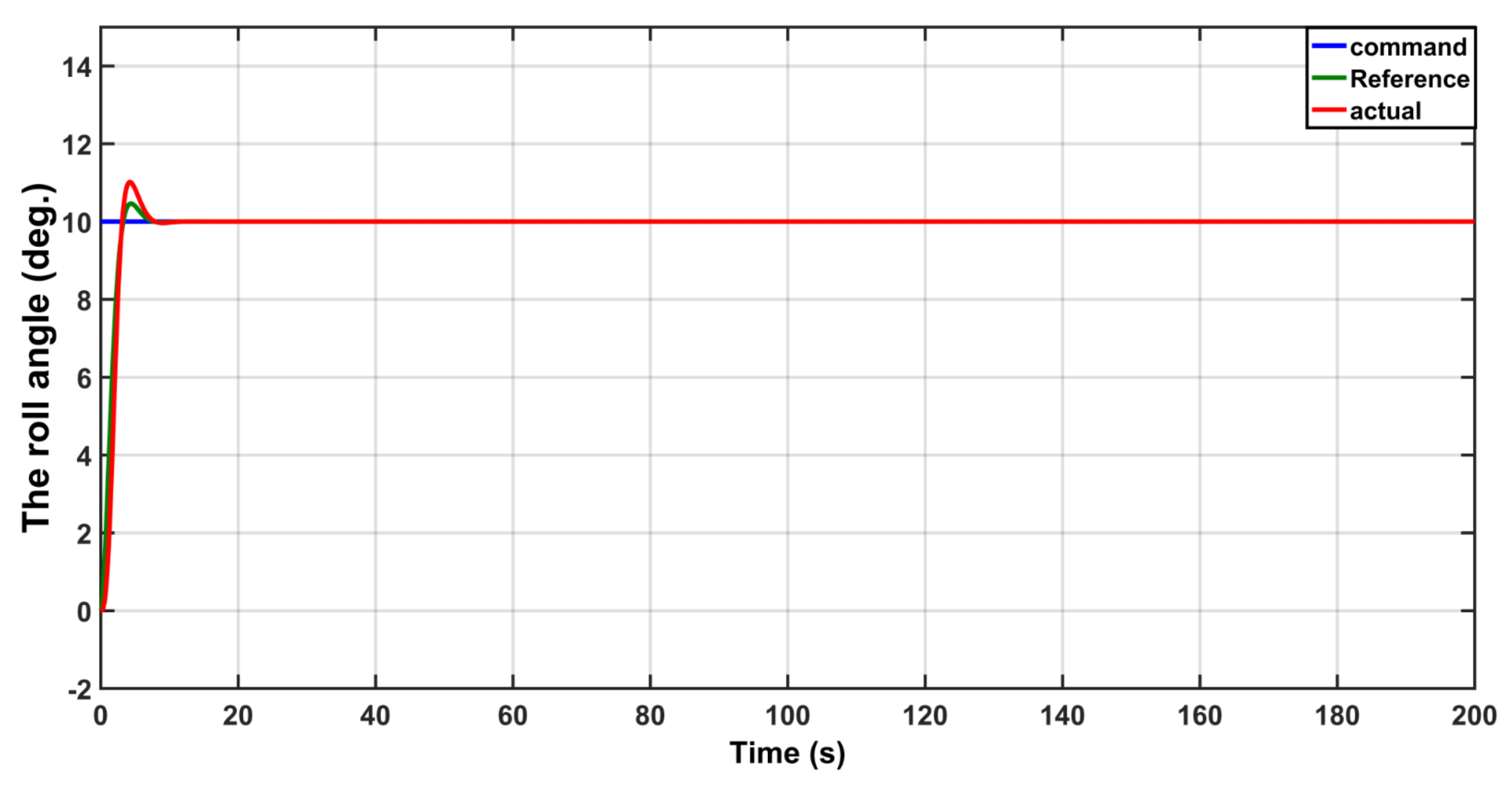
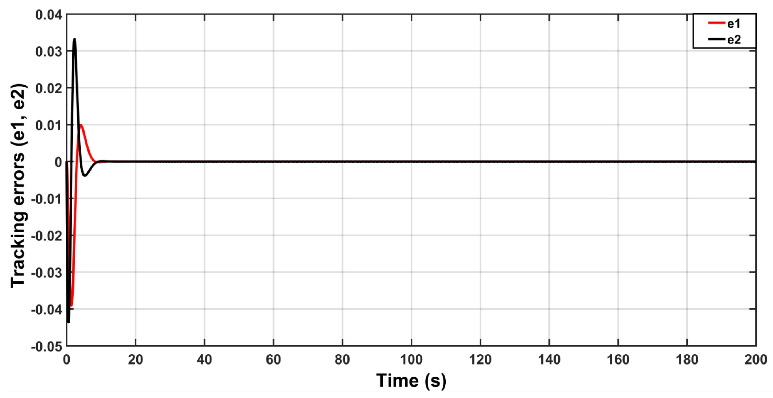
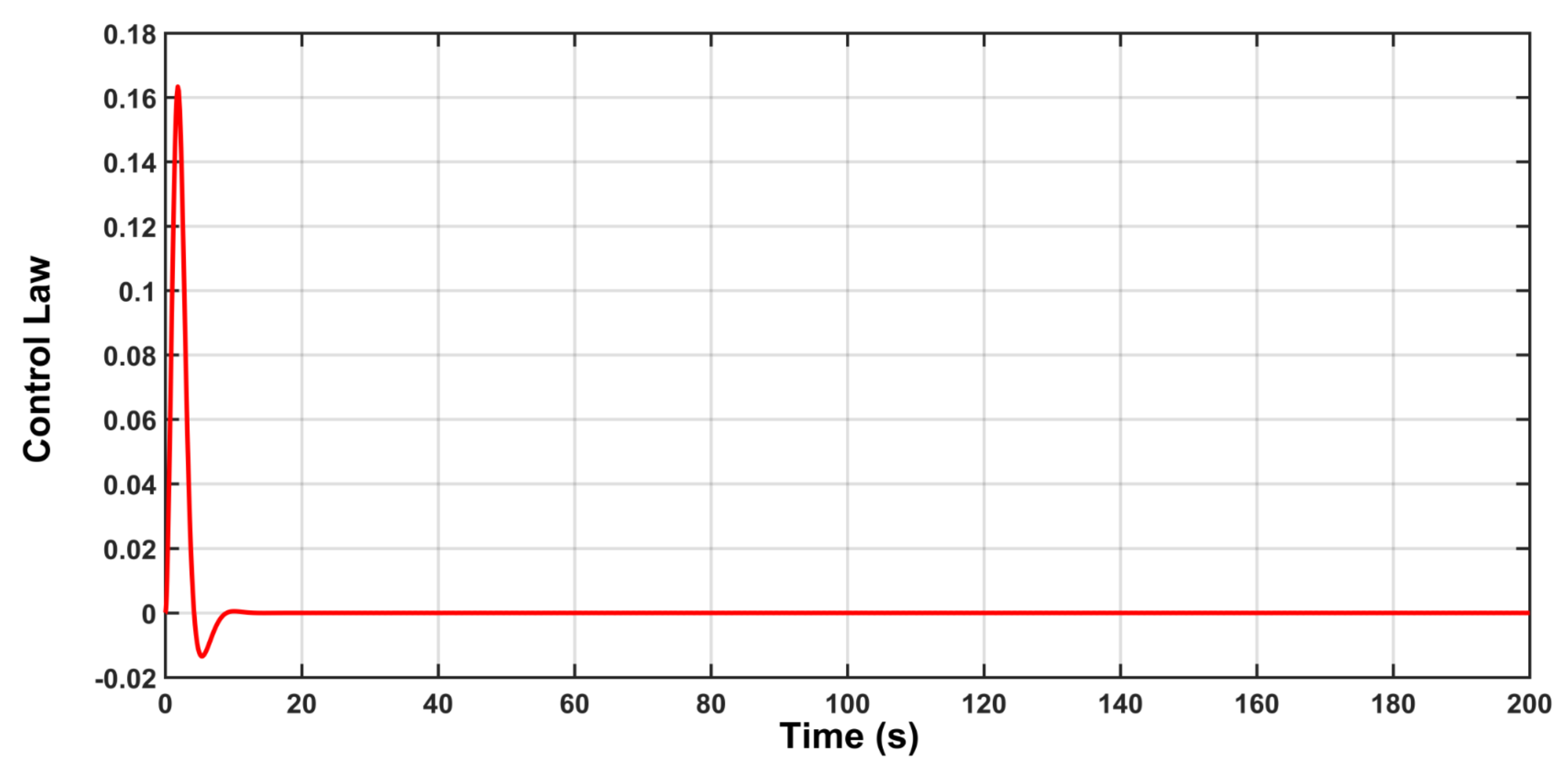
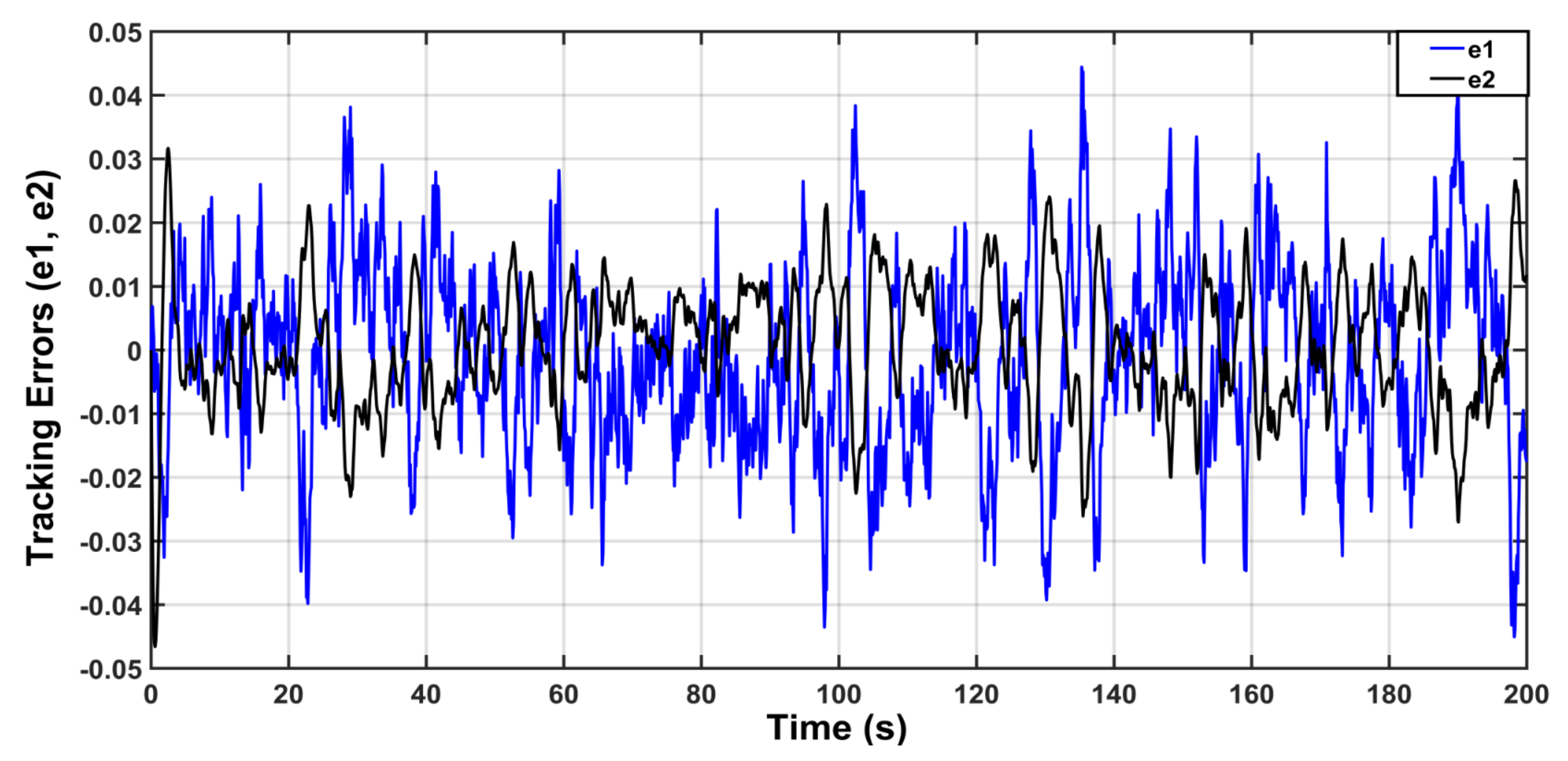
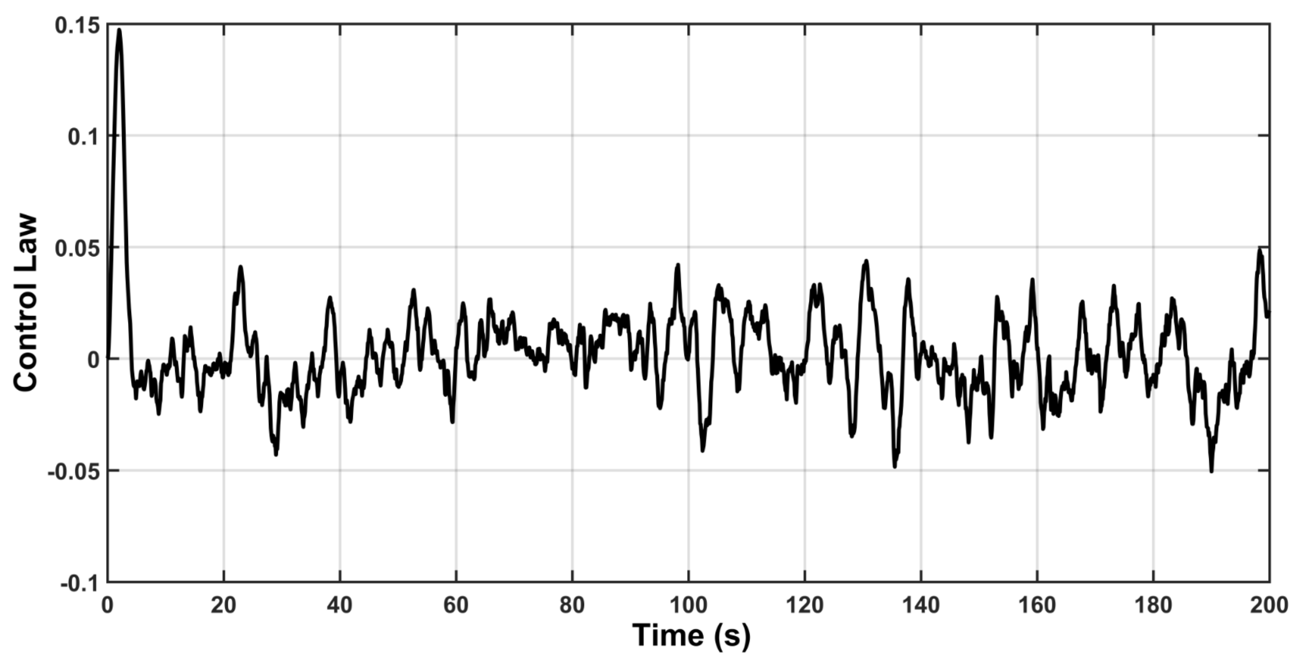
In this case, the aircraft is assumed to be free from any noise, disturbance or uncertainty. Figure 5 shows the roll angle behavior of the aircraft under this situation. It is evident that the roll angle of aircraft will follow the model reference in good manner. The behavior errors (, ) are shown in Figure 6, where represents the difference between the reference input and the model reference output, while the is the difference between the model reference output and the aircraft response. Figure 7 shows the behavior of the control law under this situation.
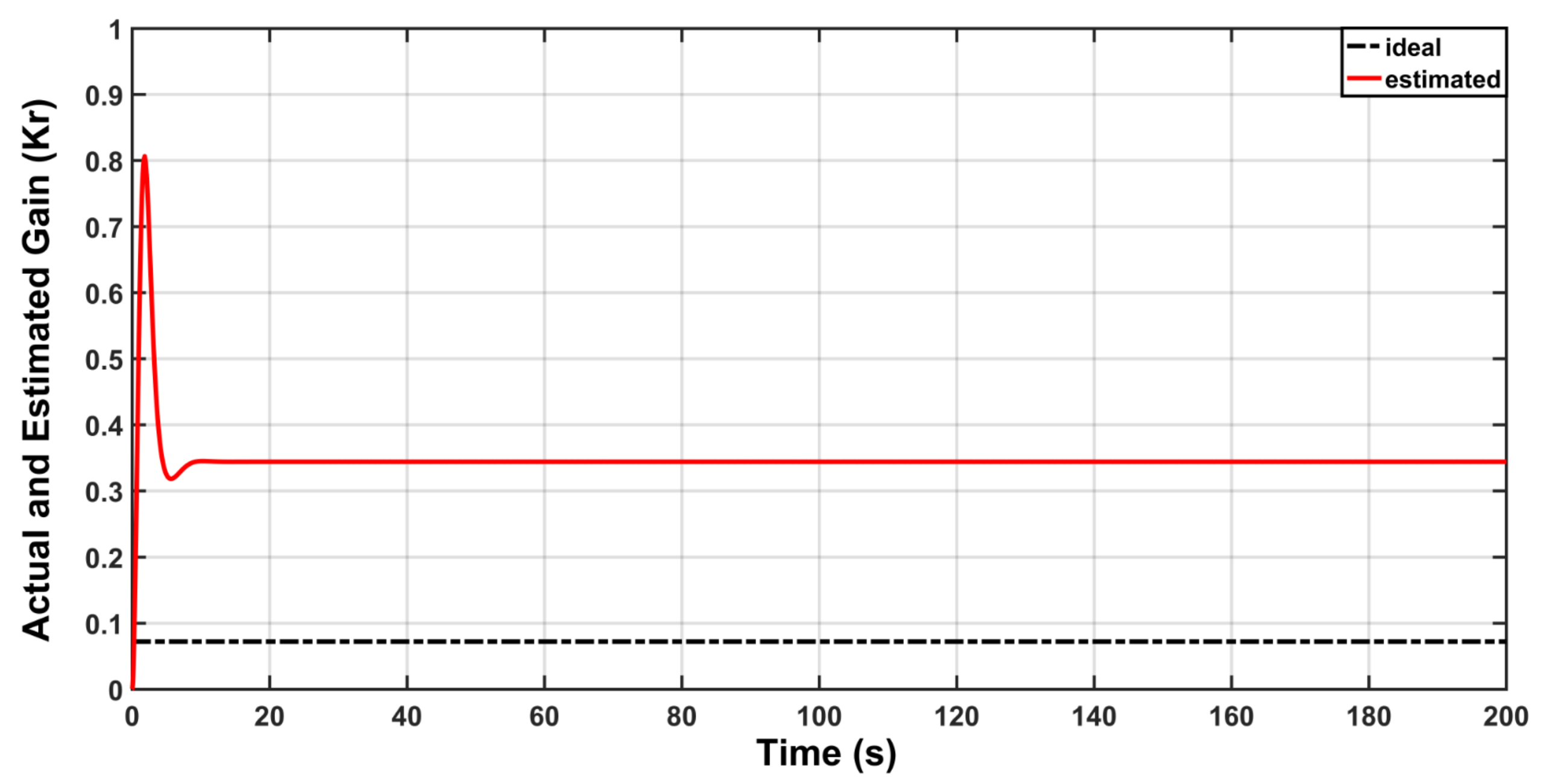
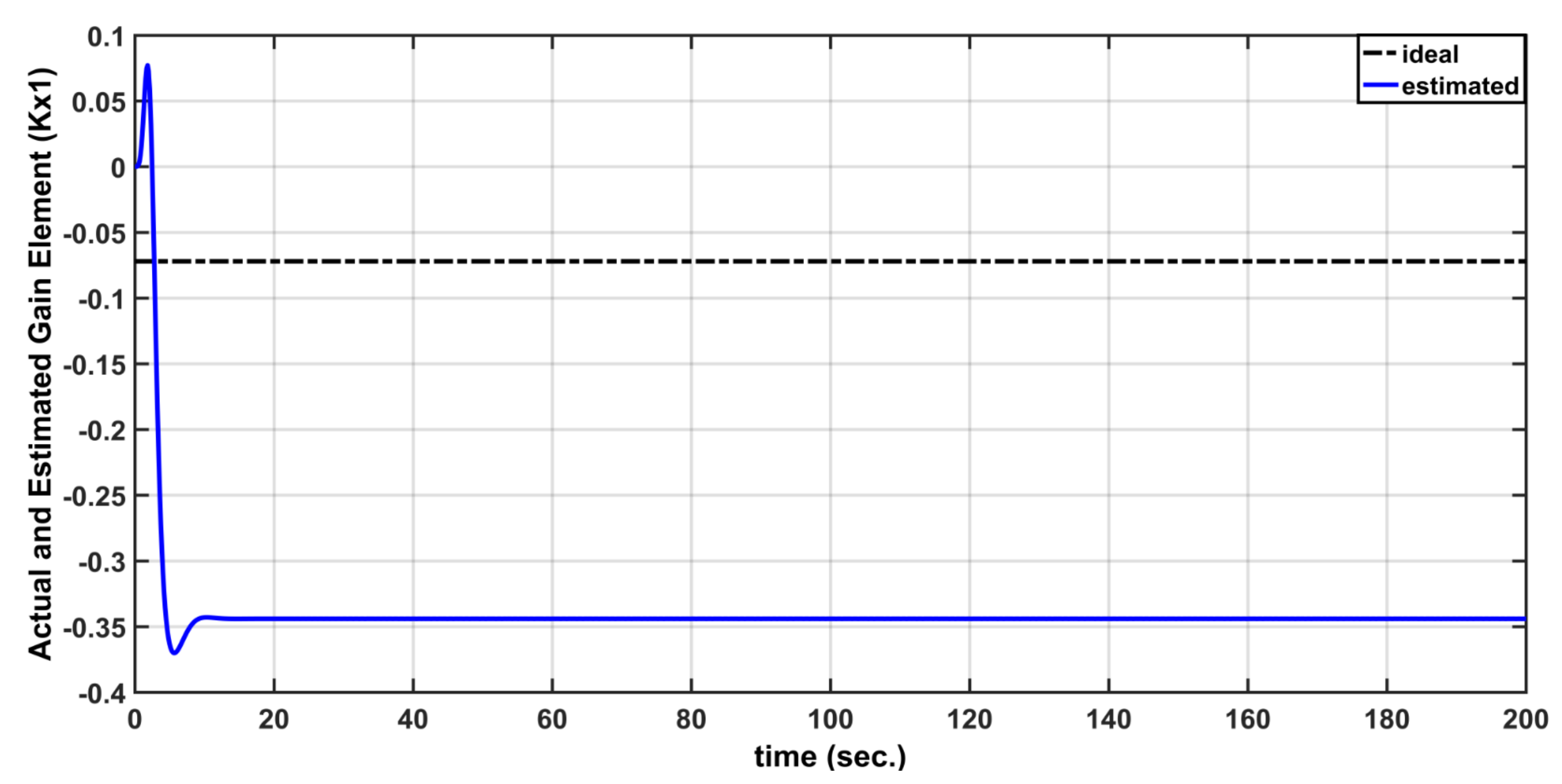
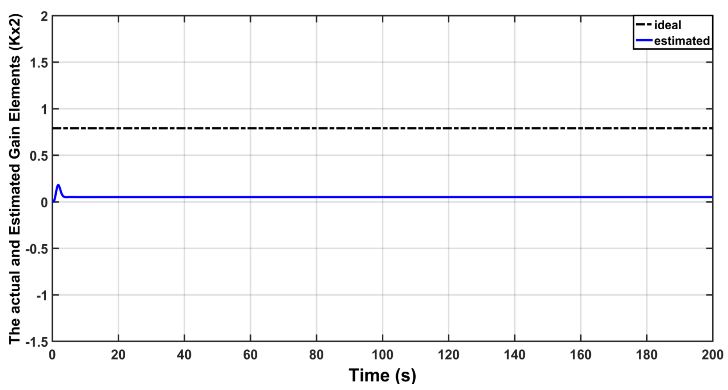
The behavior of gain matrix is illustrated in Figure 8. Also, the behavior of matrix elements (, ) are shown in Figure 9 and Figure 10. It is evident from the gain traces that the estimation errors are bounded and the adaptive controller could successfully prevent the estimation errors from drifting.
5.2. Scenario II: Uncertainty Case
In this case, it is assumed that the aircraft is subjected to rotational gust behavior, which represents a nonparametric uncertainty. The rotational gust component was modeled as a random process noise, uniformly distributed on the interval .
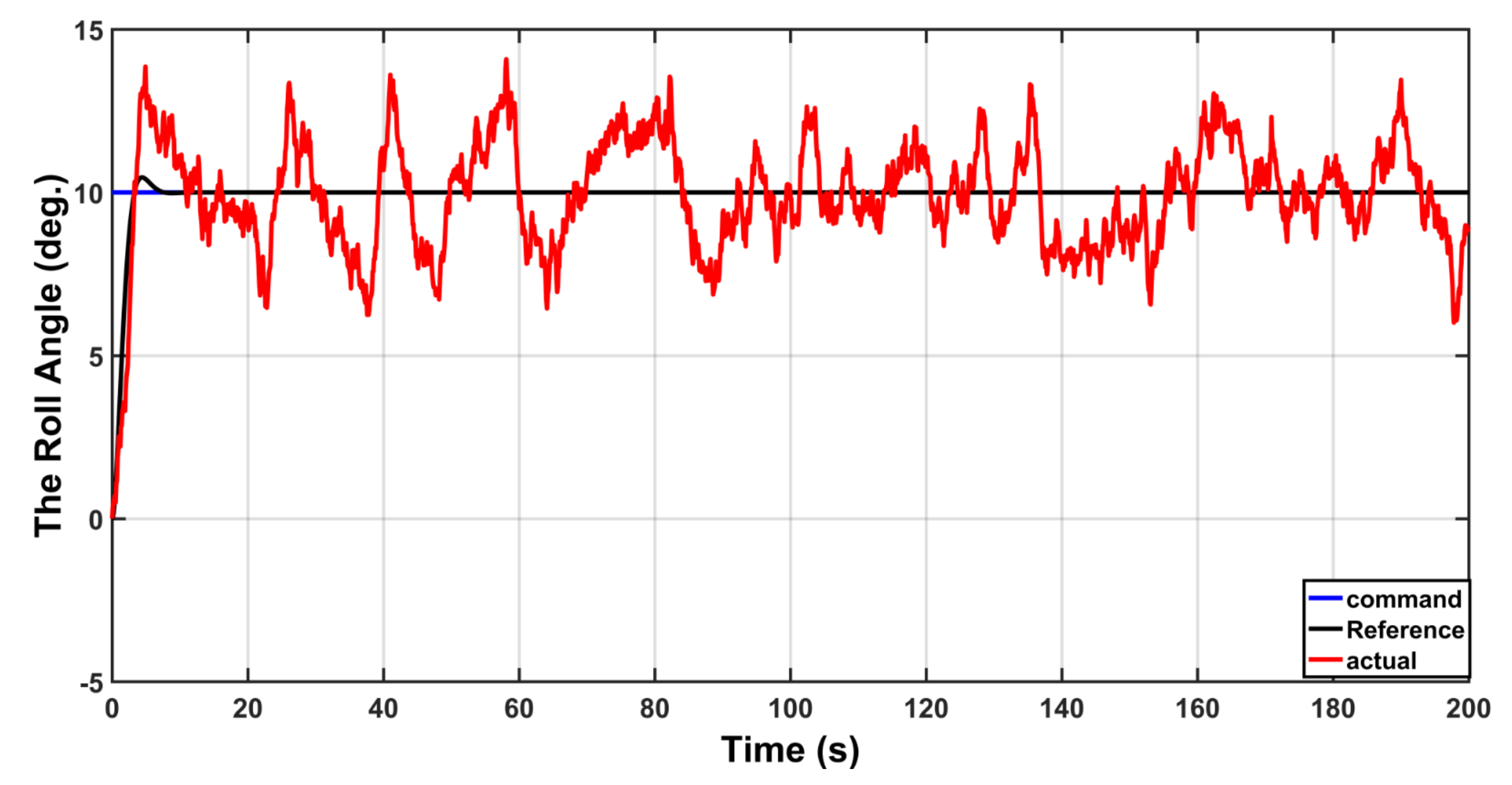
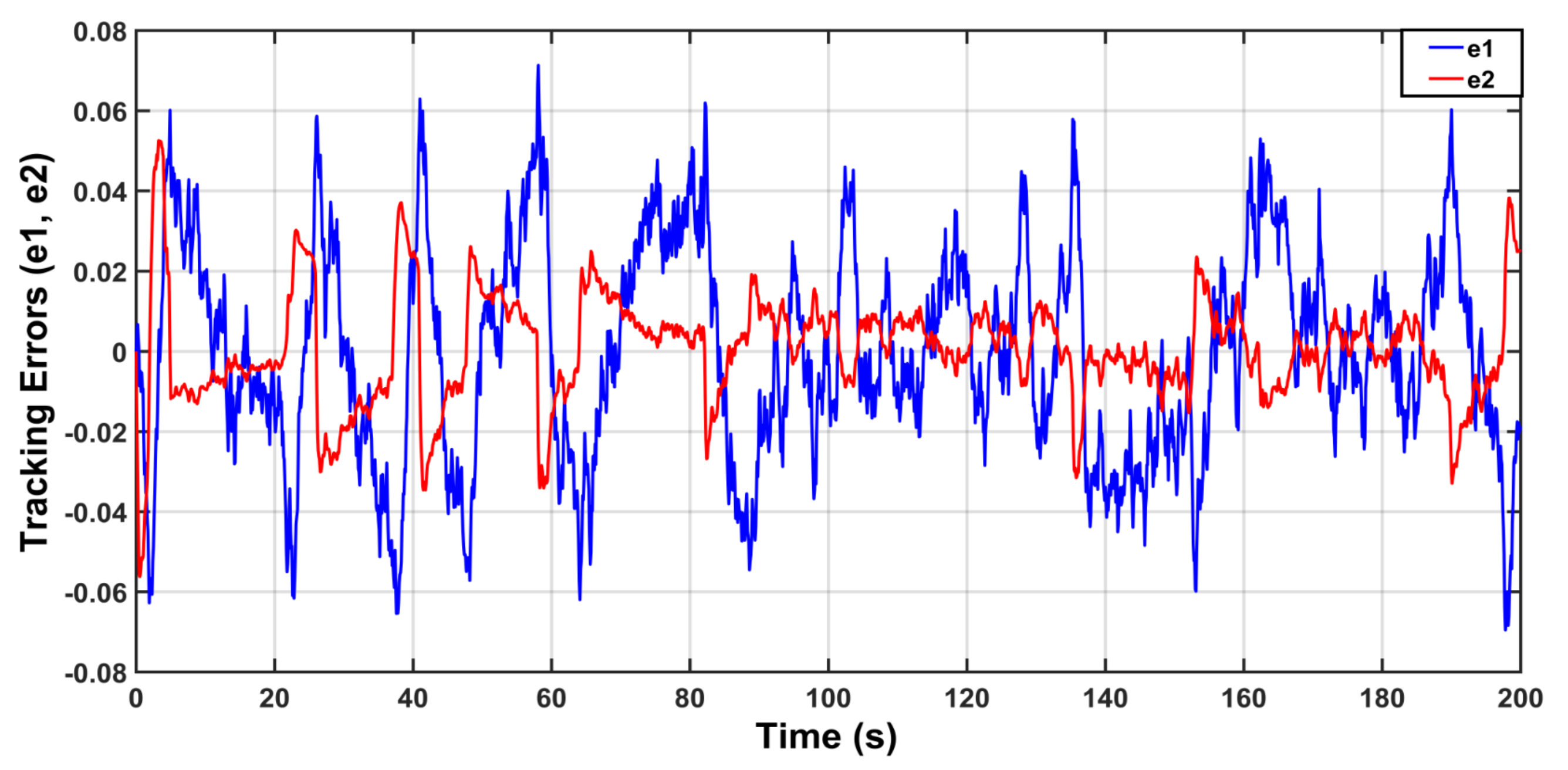
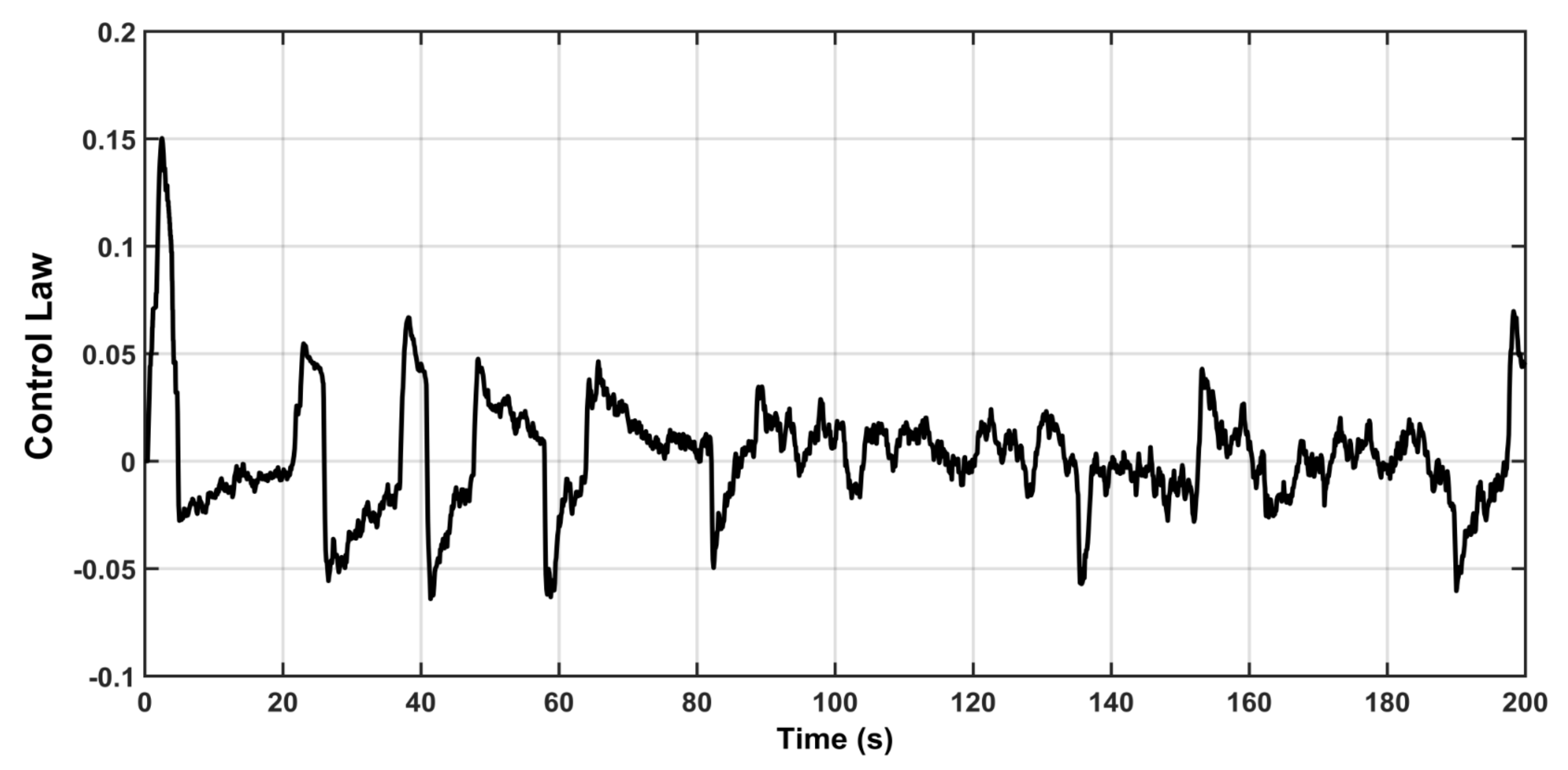
The behavior of the aircraft roll angle under gust uncertainty is shown in Figure 11. The responses of tracking errors (, ) are shown in Figure 12. The behavior of the control law resulting from this situation is illustrated in Figure 13.
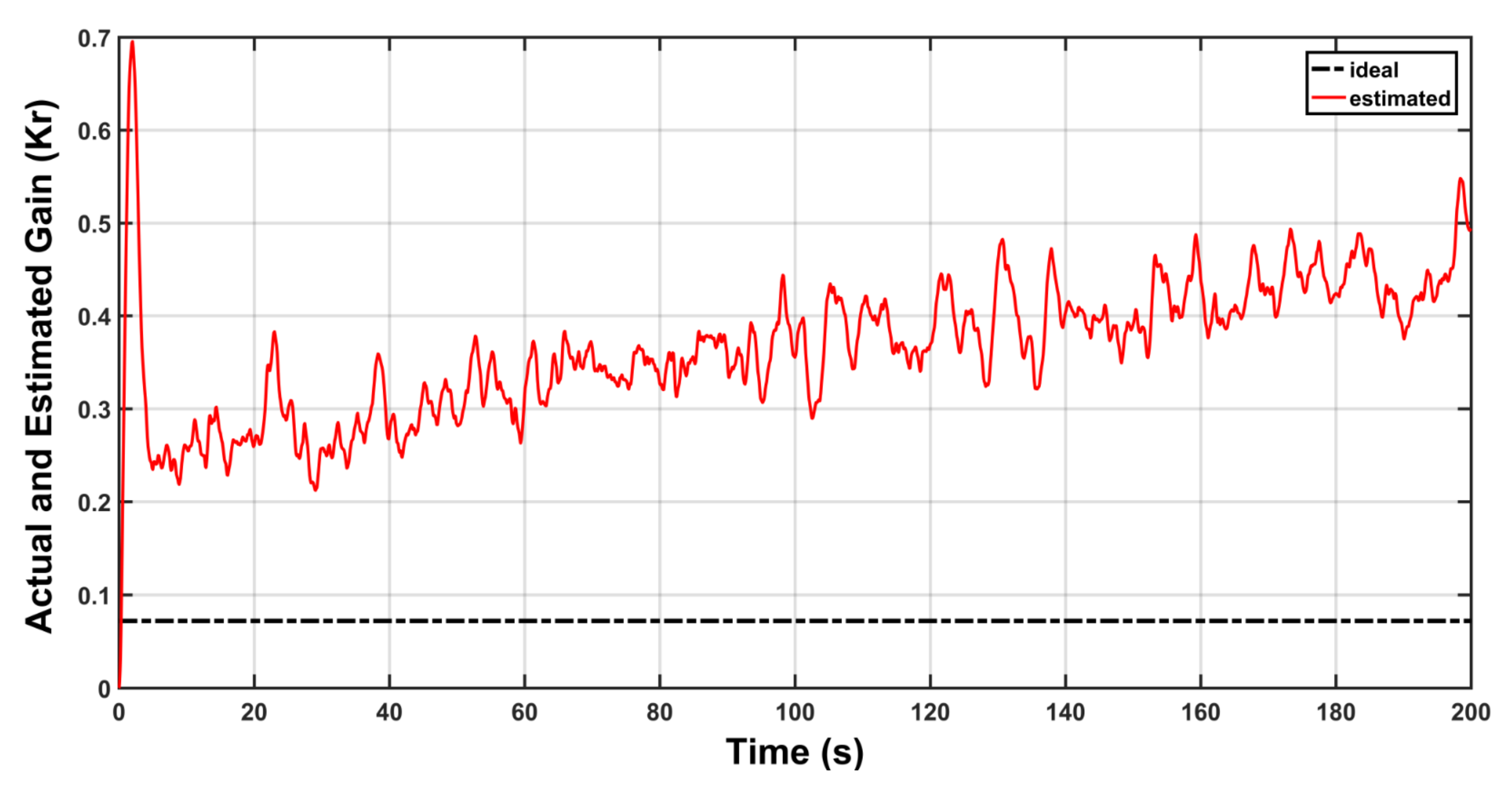
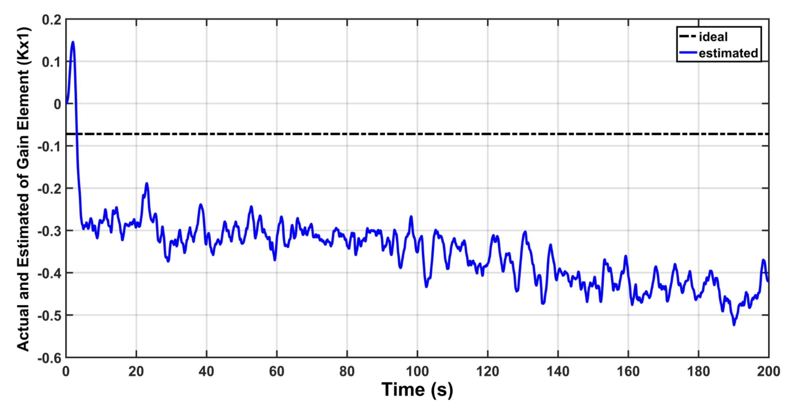
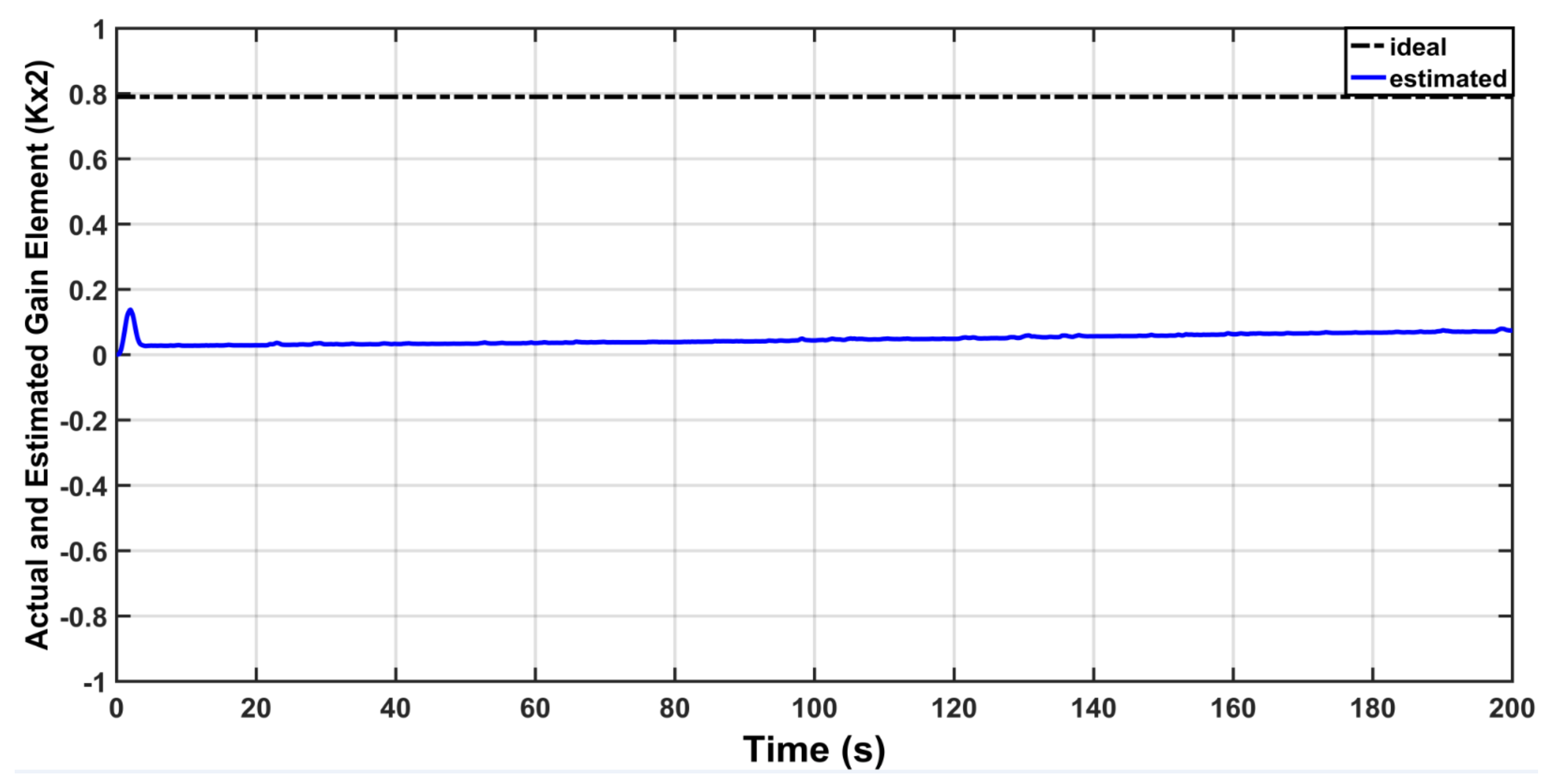
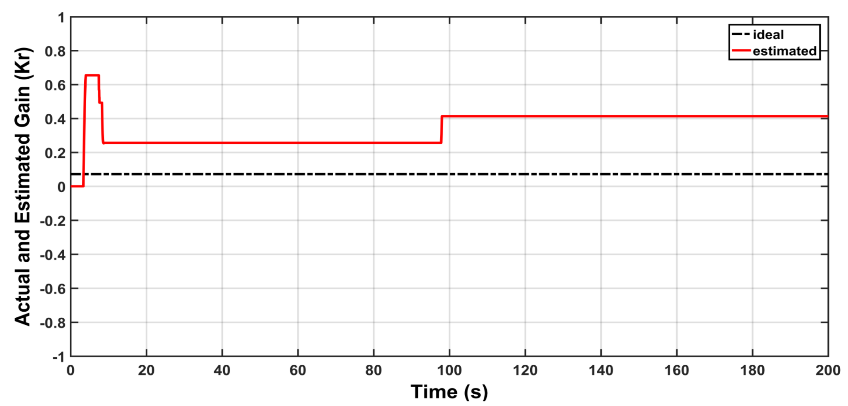
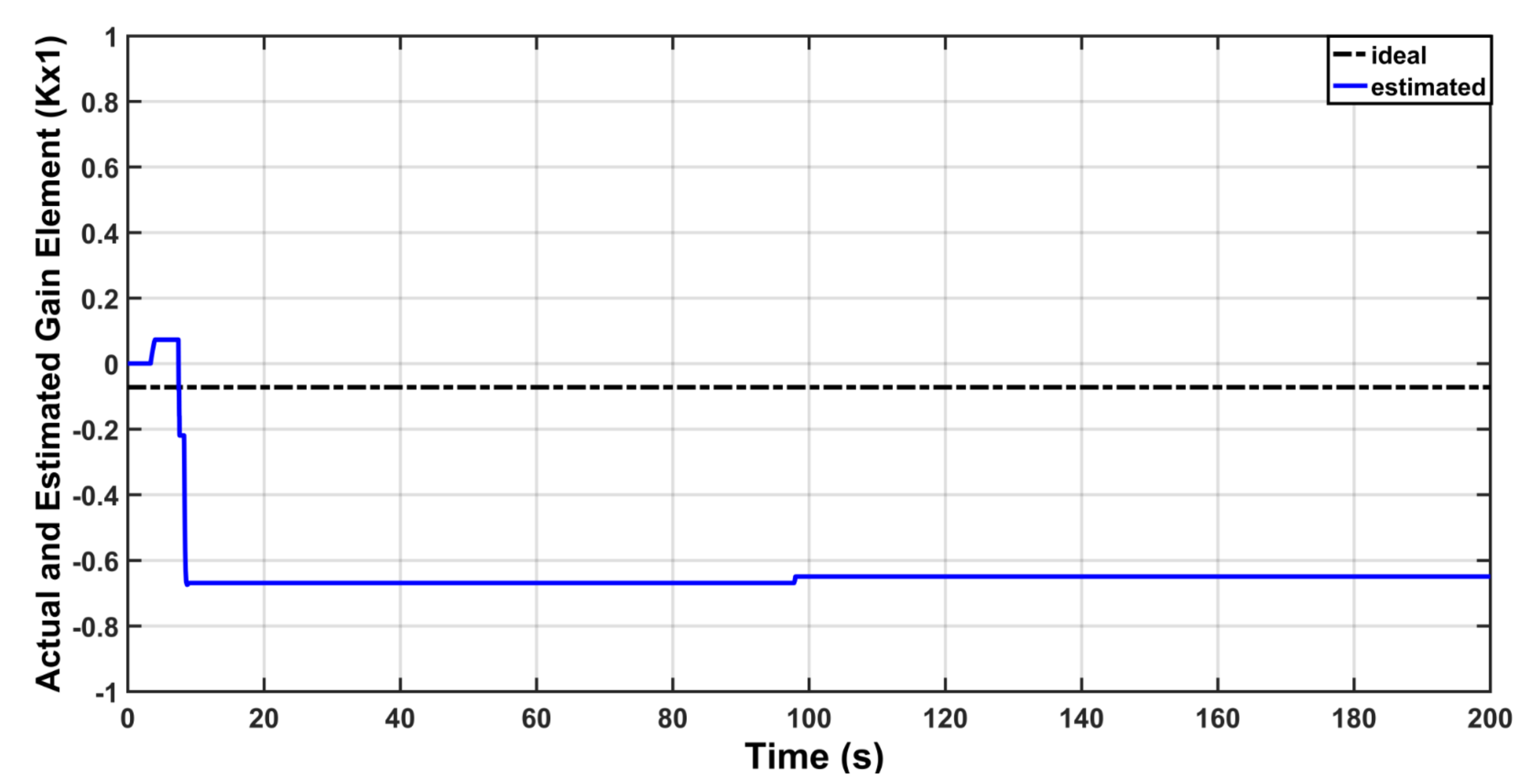
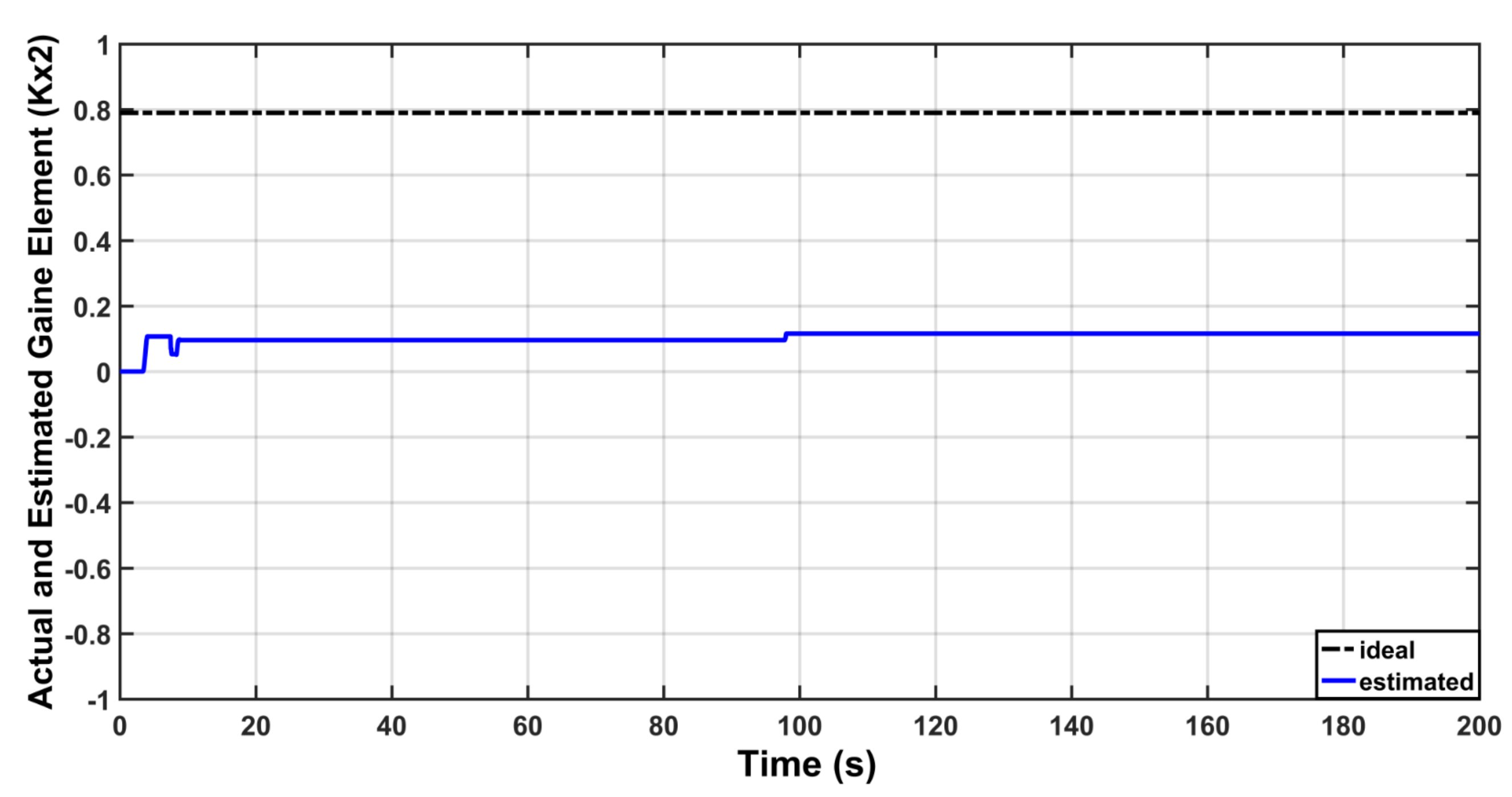
The response of feed-forward gain is depicted in Figure 14, while the behaviors of and are shown in Figure 15 and Figure 16, respectively. It is evident from the figures that there is a drift in behaviors of , and when the time goes on. In other words, the value of these gains grows without bound and this could lead to instability problems. The reason behind this is the presence of uncertainty .
5.3. Scenario III: Uncertainty with Modification
To solve the problem of drifting, which may lead to instability problems, the modification is introduced. The proposed dead-zone modification will work by stopping or avoiding the drifting. The results of this scenario are based on the inclusion of the modification. The angular position of the aircraft in the presence of uncertainty with modification is shown in Figure 14. The tracking errors are shown in Figure 15. The responses of , and are shown in Figure 16, Figure 17 and Figure 18, respectively. One can see that the drifting in feedback and feed-forward gains has been stopped in favor of the dead-zone modification.
Figure 19 shows the control signal based on modified adaptive law. The behaviors of estimated gains , and are shown in Figure 20, Figure 21 and Figure 22, respectively. It is clear from these figures that all estimated gains are bounded based on proposed modification in adaptive laws. However, this was not the case with previous scenario, where some of these gains are increasing without bound. According to this observation, the robustness of MRAC has been proved.
6. Conclusions
This work presented the design of a robust adaptive model reference controller for Tail-Sitter VTOL aircraft. The Lyapunov stability analysis of controlled aircraft based on MRAC has been conducted and the adaptive laws are developed. In the course of stability analysis, the UUB of tracking errors has been proven. The inclusion of a modification in adaptive control could guarantee the UUB of all signals and lead to robust MRAC, such that the drifting in adaptive parameters is prevented. The computer simulation has shown that the uncertainty imposed on the aircraft due to gust wind could lead to drift in the adaptive gains. However, the inclusion of dead-zone modification within the adaptive law could prevent these gains from drifting and hence robust MRAC can be obtained. This study can be extended for future work by invoking the proposed controller for three dimensional space such that the 3D dynamic model is completely utilized. Other adaptive schemes can be followed to develop the control design for the VTOL aircraft [34,35,36,37,38,39,40,41]. In addition, the MRAC design can be repeated by incorporating an appropriate filtering process, which is fused into the control design procedure for improving the control system performance in terms of noise rejection capability [42,43,44,45].
Author Contributions
Conceptualization and methodology, A.R.A.; software and analysis, A.J.H.; writing, I.K.I.; supervision and administration, A.T.A. All authors have read and agreed to the published version of the manuscript.
Funding
This research has been funded by authors.
Conflicts of Interest
The authors declare no conflict of interest.
References
- Saeeda, A.; Younesb, A.; Caic, C.; Caid, G. A Survey of Hybrid Unmanned Aerial Vehicles. Prog. Aerosp. Sci. 2018, 98, 98–105. [Google Scholar] [CrossRef]
- Guerrero, A.; Lozano, R. Flight Formation Control; ISTE, Wiley: London, UK, 2012. [Google Scholar]
- Barth, J.; Condomines, J.; Bronz, M.; Moschetta, J.; Join, C.; Fliess, M. Model-free control algorithms for micro air vehicles with transitioning flight capabilities. Int. J. Micro Air Veh. 2020, 12, 1–22. [Google Scholar] [CrossRef]
- Zhou, W.; Li, B.; Sun, J.; Wen, C.Y.; Chen, C.K. Position control of a tail-sitter UAV using successive linearization based model predictive control. Control. Eng. Pract. 2019, 91, 104125. [Google Scholar] [CrossRef]
- Wang, W.; Zhu, J.; Kuang, M.; Yuan, X.; Tang, Y.; Lai, Y.; Chen, L.; Yang, Y. Design and hovering control of a twin rotor tail-sitter UAV. Sci. China Inf. Sci. 2019, 62, 194202. [Google Scholar] [CrossRef] [Green Version]
- Nieto, S.; Carrau, J.; Valles, F.; Salcedo, J.; Simarro, R. Motion Equations and Attitude Control in the Vertical Flight of a VTOL Bi-Rotor UAV. Electronics 2019, 8, 208. [Google Scholar] [CrossRef] [Green Version]
- Ge, Z.; Hou, J. Design of the Control Law of Longitudinal Attitude for Tail-Sitter UAV. In Proceedings of the 2019 9th International Conference on Applied Physics and Mathematics (ICAPM 2019), Bangkok, Thailand, 21–23 January 2019. [Google Scholar]
- Abrougui, H.; Nejim, S.; Dallagi, H. Roll Control of a Tail-Sitter VTOL UAV. Int. J. Control Energy Electr. Eng. (CEEE) 2019, 7, 22–27. [Google Scholar]
- Flores, A.; Montes, A.; Flores, G. A Simple Controller for the Transition Maneuver of a Tail-Sitter Drone. In Proceedings of the IEEE Conference on Decision and Control (CDC), Miami Beach, FL, USA, 17–19 December 2018. [Google Scholar]
- Garcia, O.; Sanchez, A.; Escareño, J.; Lozano, R. Tail-Sitter UAV Having One Tilting Rotor: Modeling, Control and Real-Time Experiments. In Proceedings of the 17th World Congress, International Federation of Automatic Control, Seoul, Korea, 6–11 July 2008. [Google Scholar]
- Verling, S.; Weibel, B.; Boosfeld, M.; Alexis, K.; Burri, M.; Siegwart, R. Full Attitude Control of a VTOL Tail-Sitter UAV. In Proceedings of the IEEE International Conference on Robotics and Automation (ICRA), Stockholm, Sweden, 16–21 May 2016. [Google Scholar]
- Li, B.; Zhou, W.; Sun, J.; Wen, C.; Chen, C. Development of Model Predictive Controller for a Tail-Sitter VTOL UAV in Hover Flight. Sensors 2018, 18, 2859. [Google Scholar] [CrossRef] [PubMed] [Green Version]
- Çakici, F.; Kemal, M. Control System Design of a Vertical Take-off and Landing Fixed-Wing UAV. Int. Fed. Autom. Control 2016, 49, 267–272. [Google Scholar] [CrossRef]
- Astrom, K.; Wittenmark, B. Computer Controlled Systems; Prentice-Hall: Hoboken, NJ, USA, 1998. [Google Scholar]
- Nguyen, T. Model-Reference Adaptive Control; Springer International Publishing AG: Cham, Switzerland, 2018. [Google Scholar]
- Humaidi, A.; Hameed, M. Development of a New Adaptive Backstepping Control Design for a Non-Strict and Under-Actuated System Based on a PSO Tuner. Inf. J. 2019, 10, 38. [Google Scholar] [CrossRef] [Green Version]
- Shekhar, A.; Sharma, A. Review of Model Reference Adaptive Control. In Proceedings of the IEEE, International Conference on Information, Communication, Engineering and Technology (ICICET), Pune, India, 29–31 August 2018. [Google Scholar]
- Humaidi, A.J.; Hasan, A.F. Particle swarm optimization–based adaptive super-twisting sliding mode control design for 2-degree-of-freedom helicopter. Sage Meas. Control J. 2019, 9/10, 1403–1419. [Google Scholar] [CrossRef] [Green Version]
- Humaidi, A.J.; Ibraheem, I.K.; Azar, A.T.; Sadiq, M.E. A New Adaptive Synergetic Control Design for Single Link Robot Arm Actuated by Pneumatic Muscles. Entropy 2020, 227, 723. [Google Scholar] [CrossRef] [PubMed]
- Bierling, T. Comparative Analysis of Adaptive Control Techniques for Improved Robust Performance. Ph.D. Thesis, Technical University of Munich, Munich, Germany, 2015. [Google Scholar]
- Amjad, J.H.; Akram, H.H.; Mustafa, R.H. Robust Adaptive Speed Control for DC Motor Using Novel Weighted E-Modified MRAC. In Proceedings of the IEEE International Conference on Power, Control, Signals and Instrumentation Engineering (ICPCSI), Chennai, India, 21–22 September 2017. [Google Scholar]
- Zhao, X.; Guo, G. Model Reference Adaptive Control of Vehicle Slip Ratio Based on Speed Tracking. Appl. Sci. 2020, 10, 3459. [Google Scholar] [CrossRef]
- Trajkov, T.; Köppe, H.; Gabbert, U. Direct model reference adaptive control (MRAC) design and simulation for the vibration suppression of piezoelectric smart structures. Commun. Nonlinear Sci. Numer. Simul. 2007, 13, 1896–1909. [Google Scholar] [CrossRef]
- Balaska, H.; Ladaci, S.; Schulte, H.; Djouambi, A. Adaptive Cruise Control System for an Electric Vehicle Using a Fractional Order Model Reference Adaptive Strategy. In Proceedings of the 9th IFAC Conference on Manufacturing Modelling, Management and Control, Berlin, Germany, 28–30 August 2019. [Google Scholar]
- Humaidi, A.; Hameed, A. Robustness enhancement of MRAC using modification techniques for speed control of three phase induction motor. J. Electr. Syst. 2017, 13, 723–741. [Google Scholar]
- Stepanyan, V.; Kumar, K. Adaptive Control with Reference Model Modification. J. Guid. Control. Dyn. 2012, 35, 1370–1374. [Google Scholar] [CrossRef] [Green Version]
- Zareh, M.; Soheili, S. A modified model reference adaptive control with application to MEMS gyroscope. J. Mech. Sci. Technol. 2011, 25, 1–7. [Google Scholar] [CrossRef]
- Rothe, J.; Zevering, J.; Strohmeier, M.; Montenegro, S. A Modified Model Reference Adaptive Controller (M-MRAC) Using an Updated MIT-Rule for the Altitude of a UAV. Electronics 2020, 9, 1104. [Google Scholar] [CrossRef]
- Humaidi, A.; Hameed, A. PMLSM position control based on continuous projection adaptive sliding mode controller. Syst. Sci. Control. Eng. 2018, 6, 242–252. [Google Scholar] [CrossRef]
- Wong, K.; Guerrero, J.; Lara, D.; Lozano, R. Attitude Stabilization in Hover Flight of a Mini Tail-Sitter UAV with Variable Pitch Propeller. In Proceedings of the/RSJ International Conference on Intelligent Robots and Systems, San Diego, CA, USA, 29 October–2 November 2007. [Google Scholar]
- Stevens, B.; Lewis, F.; Johnson, E. Aircraft Control and Simulation: Dynamics, Controls Design, and Autonomous Systems, 3rd ed.; John Wiley & Sons Inc.: Hoboken, NJ, USA, 2016. [Google Scholar]
- Lavretsky, E.; Wise, K. Robust and Adaptive Control; Springer: London, UK, 2013. [Google Scholar]
- Slotine, J.-J.E.; Coetsee, J.A. Adaptive sliding controller synthesis for nonlinear systems. Int. J. Control 1986, 43, 1631–1651. [Google Scholar] [CrossRef]
- Jaleel, A.H.; Hameed, M.R.; Hameed, A.H. Design of Block-Bakstepping Controller to Ball and Arc System Based on Zero Dynamic Theory. J. Eng. Sci. Technol. 2018, 13, 2084–2105. [Google Scholar]
- Radac, M.B.; Borlea, A.I. Virtual State Feedback Reference Tuning and Value Iteration Reinforcement Learning for Unknown Observable Systems Control. Energies 2021, 14, 1006. [Google Scholar] [CrossRef]
- Al-Dujaili, A.Q.; Falah, A.; Humaidi, A.J.; Pereira, D.A.; Ibraheem, I.K. Optimal super-twisting sliding mode control design of robot manipulator: Design and comparison study. Int. J. Adv. Robot. Syst. 2020, 17, 172988142098152. [Google Scholar] [CrossRef]
- Fu, H.; Chen, X.; Wang, W.; Wu, M. MRAC for unknown discrete-time nonlinear systems based on supervised neural dynamic programming. Neuro Comput. 2020, 384, 130–141. [Google Scholar] [CrossRef]
- Yuksek, B.; Inalhan, G. Reinforcement learning based closed-loop reference model adaptive flight control system design. Int. J. Adapt. Control Signal Process. 2021, 35, 420–440. [Google Scholar] [CrossRef]
- Amjad, J.H.; Badr, H.M.; Ajil, A.R. Design of Active Disturbance Rejection Control for Single-Link Flexible Joint Robot Manipulator. In Proceedings of the IEEE, 2018 22nd International Conference on System Theory, Control and Computing (ICSTCC), Sinaia, Romania, 10–12 October 2018. [Google Scholar]
- Sands, T. Comparison and Interpretation Methods for Predictive Control of Mechanics. Algorithms 2019, 12, 232. [Google Scholar] [CrossRef] [Green Version]
- Humaidi, A.J.; Hussein, H.A. Adaptive Control of Parallel Manipulator in Cartesian space. In Proceedings of the IEEE International Conference on Electrical, Computer and Communication Technologies (ICECCT), Coimbatore, India, 20–22 February 2019. [Google Scholar]
- Shi, Y.; Fang, H.; Yan, M. Kalman filter-based adaptive control for networked systems with unknown parameters and randomly missing outputs. Int. J. Robust Nonlinear Control 2009, 19, 1976–1992. [Google Scholar] [CrossRef]
- Zirkohi, M.M. Command filtering-based adaptive control for chaotic permanent magnet synchronous motors considering practical considerations. ISA Trans. 2020, 114, 120–135. [Google Scholar] [CrossRef]
- Humaidi, A.J.; Ibraheem, I.K.; Ajel, A.R. A Novel Adaptive LMS Algorithm with Genetic Search Capabilities for System Identification of Adaptive FIR and IIR Filters. Inf. J. 2019, 10, 176. [Google Scholar] [CrossRef] [Green Version]
- Yuan, J.; Li, J.; Zhang, A.; Zhang, X.; Ran, J. Active Noise Control System Based on the Improved Equation Error Model. Acoustics 2021, 3, 354–363. [Google Scholar] [CrossRef]
Figure 1.
(a) The real Tail-Sitter UAV (b) Flight Dynamics.

Figure 2.
The Configuration of roll dynamics.

Figure 3.
Lipschitz-continuous dead-zone function.

Figure 4.
Schematic diagram of robust MRAC for Tail-Sitter Aircraft.

Figure 5.
Behavior of the roll angle.

Figure 6.
Behavior of tracking errors.

Figure 7.
The control response with an uncertainty-free case.

Figure 8.
Actual and Estimated behavior of .

Figure 9.
Actual and Estimated behavior of .

Figure 10.
Actual and Estimated behavior of .

Figure 11.
Behavior of the roll angle.

Figure 12.
Behavior of tracking errors.

Figure 13.
The control response with gust uncertainty.

Figure 14.
Actual and Estimated behavior of .

Figure 15.
Actual and Estimated behavior of .

Figure 16.
Actual and Estimated behavior of .

Figure 17.
Behavior of the roll angle.

Figure 18.
Behaviors of tracking errors.

Figure 19.
The response of control with uncertainty.

Figure 20.
Actual and Estimated behavior of .

Figure 21.
Actual and Estimated behavior of .

Figure 22.
Actual and Estimated behavior of .


Table 1.
Numeric parameters of Tail-Sitter VTOL Aircraft.
| Parameter | Description | Value |
|---|---|---|
| x-axis moment of inertia | ||
| Roll damping coefficient | 0.36 | |
| Rotor distance from the center of mass |
Publisher’s Note: MDPI stays neutral with regard to jurisdictional claims in published maps and institutional affiliations. |
© 2021 by the authors. Licensee MDPI, Basel, Switzerland. This article is an open access article distributed under the terms and conditions of the Creative Commons Attribution (CC BY) license (https://creativecommons.org/licenses/by/4.0/).
Share and Cite
MDPI and ACS Style
Ajel, A.R.; Humaidi, A.J.; Ibraheem, I.K.; Azar, A.T. Robust Model Reference Adaptive Control for Tail-Sitter VTOL Aircraft. Actuators 2021, 10, 162. https://0-doi-org.brum.beds.ac.uk/10.3390/act10070162
AMA Style
Ajel AR, Humaidi AJ, Ibraheem IK, Azar AT. Robust Model Reference Adaptive Control for Tail-Sitter VTOL Aircraft. Actuators. 2021; 10(7):162. https://0-doi-org.brum.beds.ac.uk/10.3390/act10070162
Chicago/Turabian StyleAjel, Ahmed R., Amjad J. Humaidi, Ibraheem Kasim Ibraheem, and Ahmad Taher Azar. 2021. "Robust Model Reference Adaptive Control for Tail-Sitter VTOL Aircraft" Actuators 10, no. 7: 162. https://0-doi-org.brum.beds.ac.uk/10.3390/act10070162
Note that from the first issue of 2016, this journal uses article numbers instead of page numbers. See further details here.