Delay-Dependent Stability Analysis of Haptic Systems via an Auxiliary Function-Based Integral Inequality

Abstract

In this paper, the delay-dependent stability of haptic systems is studied by developing a new stability criterion. Firstly, the haptic system inevitably introduces time delays by using communication networks to transmit information between the controller and the haptic device. When discussing the stability of the haptic system near its operating point, the original nonlinear system is modeled as a linear system with the time delay mentioned above. In addition, a suitable augmented Lyapunov–Krasovskii functional (LKF) with more integral forms is constructed and an auxiliary function-based integral inequality is applied to estimate the derivative of the proposed LKF. Then, a less conservative delay-dependent criterion in terms of the linear matrix inequality (LMI) is derived to calculate the delay margin for the haptic system. Finally, case studies are carried out based on a one degree of freedom haptic system. The results show that, compared with criteria in existing works, the proposed criterion can obtain more accurate results and require less calculation complexity, and, with the increase in virtual damping in a certain range, the stable upper bound of the haptic system increases at first and then decreases.

1. Introduction

Haptic devices are widely used in virtual reality systems, such as virtual prototyping [1], teleoperation [2] and human–robot interaction [3]. The haptic system utilizes communication networks to transmit information between the controller and the haptic device, inevitably including time delays [4,5]. These delays degrade the dynamic performance of haptic devices and can even hurt their operator. Thus, time delays should be taken into account for stability analysis of haptic systems.

The previous research, in stability analysis of haptic systems, can be divided into two categories, frequency-domain methods and time-domain methods. By employing the frequency-domain method, the stability of haptic systems was firstly studied by Minsky et al. [6], in which haptic devices and virtual environments were generally modeled as linear models of mass dampers and spring dampers. Then, Hannaford et al. proposed a more accurate method by introducing a passive controller stabilize the system [7,8]. Meanwhile, Gil et al. considered the time delay and derived a stability criterion by using Routh–Hurwitz and Nyquist criteria [9,10]. They put forward a new linear condition, which summarizes relationships among virtual stiffness, viscous damping and time delays. In the meanwhile, by numerically solving some complex equations, the stability boundaries with large virtual damping and large time delay were drawn. Frequency-domain methods can acquire the precise delay boundaries for a haptic system. However, they are complicated in calculating the eigenvalue of the haptic system. In order to avoid calculating eigenvalue information, time-domain methods based on Lyapunov stability theory are introduced to study the stability of haptic systems. In [4], two methods were proposed to analyze the stability of the haptic system involving the time delay. In the first method of [4], model transform was used to determine the stability boundary, which brings conservatism in the process of defining cross terms, while the second was based on the free-weighing-matrix approach, which introduced free weighting matrices to reduce conservatism of calculation results of the time delay boundary, resulting in a large number of additional decision variables. Then, Mashayekhi et al. extended the existing work of [4] by using state-space equations without parameter constraints [11]. Based on this promotion, any linear model of the operator’s hand can be introduced into the stability analysis of haptic systems. The related stability criteria used in [4,11] are conservative, which reduces the accuracy of the stability analysis. Moreover, the above criteria with relatively low conservatism show high calculation complexity, which affects the efficiency of the stability analysis. The question of how to reduce the conservatism and the calculation complexity motivates the current work.

In order to study the stability of haptic systems considering the effect of time delays, one of the keys is to obtain a stability criterion with less conservatism and less calculation complexity. For obtaining stability criteria with less conservatism, various methods have been developed in the theoretical study of time-delay systems, for example, different Lyapunov–Krasovskii functionals (LKFs) (see, e.g., augmented LKF [12], indefinite derivative LKF [13], delay-product-type LKF [14], etc.), and different methods for estimating integral terms (see, e.g., free-weighting-matrix approach [15], Wirtinger-based integral inequality [16], auxiliary function-based integral inequality [17], free-matrix-based inequality [18], extended reciprocally convex matrix inequality [19], quadratic generalized free-weighting matrix inequality [20], generalized free-matrix-based integral inequality [21], etc.). In fact, the existing methods for analyzing the stability of the haptic system show lots of conservatism to be reduced. The auxiliary function-based integral inequality in [17] is reported to give tight upper bounds. Thus, using this inequality to investigate the stability analysis of the haptic system is expected to obtain results with less conservatism for delay margins.

In this paper, the delay-dependent stability of haptic systems with time delays is further studied. A suitable augmented LKF with more integral forms is constructed and an auxiliary function-based integral inequality is applied to estimate the derivative of the proposed LKF. Then, a delay-dependent criterion with less conservatism is developed to calculate the delay margin. The main contributions of this paper are two-fold: (1) Reduce the conservatism of the stability criterion to make the calculated delay margin be more accurate; (2) Decrease the number of the decision variables in the derived criterion to reduce the computing time of delay margin calculation. Finally, case studies are considered to illustrate advantages of the proposed stability criterion.

The framework of this paper is as follows. Section 2 briefly describes the modeling process of the haptic system. Based on the time-delay system model, an augmented LKF is employed to establish a stability criterion in Section 3. In Section 4, case studies are carried out to illustrate the availability and predominance of the proposed criterion. Finally, Section 5 gives the conclusion.

Notation 1.

Throughout this paper, $R^n$ refers to the n-dimensional Euclidean space; $\parallel ·\parallel$ means the Euclidean vector norm; the superscripts T and $-1$ stand for the transpose and the inverse of a matrix, respectively; col $\{y_1,y_2,\dots ,y_n\}={[y_1^T,y_2^T,\dots ,y_n^T]}^T$; diag $\{·\}$ refer to a block-diagonal matrix and $X>0(\ge 0)$ represents that X is a positive-definite (semi-positive-definite) and symmetric matrix.

2. System Description

A haptic device is nonlinear and has multiple degrees of freedom. When the operator’s hand is in the contact with it by simulating a virtual object, the position of its contact point is always constant or may have only a small fluctuation at the stable point. In addition, the energy dissipation of the haptic system by Coulomb friction makes the system more stable. Ref. [22] showed that the energy of coulomb friction dissipation is larger than that of quantization and discretization in sensor. On this basis, the nonlinear effects caused by coulomb friction and quantization can be omitted. Hence, the dynamic model of the haptic device can be linearized near its working point, and the device is considered to be a one degree of freedom (1-DOF) system with an equivalent mass of m with b as viscous friction. A structure diagram of a 1-DOF haptic device with an operator’s hand is depicted in Figure 1 [4]. In this figure, $F_{VE}$ is the force of the virtual environment, and m, $t_d$, K, B, c and b are mass, sampling time, time delay, virtual stiffness, virtual damping, coulomb friction and viscous friction of the haptic device, respectively.

A haptic system is a sampled-data controlled device. It utilizes communication networks to transmit information between the controller and the haptic device including time delays, inevitably [4]. Time delay in the process of communication will affect the performance of the system, and even lead to instability. Therefore, the influence of time delay is important for stability analysis in haptic system. In order to simplify the analysis, as mentioned in [23], all time delays can be added up to a single time delay of $t_d$. This is because the model of the haptic device is linear.

By defining two state variables $x_1=x$ (x is the position of the haptic device) and $x_2=\dot{x}$, as in [4], using Newton’s second law and employing the results in [22,24], the whole haptic system model can be written as the following equation in state-space form:

$$\left\{\begin{array}{c}{\dot{x}}_1=x_2\hfill \\ {\dot{x}}_2=-\frac{b}{m}{x}_2-\frac{K}{m}{x}_1\left(t-t_d-\frac{T}{2}\right)-\frac{B}{m}{x}_2\left(t-t_d-T\right)\hfill \end{array}\right.$$

(1)

where T is sampling time.

Define a vector of $X={\left[x_1,x_2\right]}^T$, then the state space expression can be rewritten as:

$$\dot{X}\left(t\right)=A_{0}X(t-h_0)+A_{1}X(t-h_1)+A_{2}X(t-h_2)$$

(2)

where $h_0=0$, $h_1=T/2+t_d$, $h_2=T+t_d$ and $A_0=\left[\begin{array}{cc}0& 1\\ 0& -\frac{b}{m}\end{array}\right],A_1=\left[\begin{array}{cc}0& 0\\ -\frac{K}{m}& 0\end{array}\right],A_2=\left[\begin{array}{cc}0& 0\\ 0& -\frac{B}{m}\end{array}\right]$.

3. A Stability Criterion

This section develops a new delay-dependent stability criterion for the haptic system (2). By estimating the integral term of derivative of LKF based on an auxiliary function-based integral inequality, a result with less conservatism and calculation complexity is obtained.

Before developing the stability criterion, the following lemma is given at first.

Lemma 1

([17]). For a matrix $R>0$, scalars a and b with $b>a$, and a vector ω such that the integration concerned is well defined, the following inequality holds:

$$(b-a){\int }_a^b{\dot{\omega }}^T\left(s\right)R\dot{\omega }\left(s\right)ds\ge {\chi }_1^{T}R{\chi }_1+3{\chi }_2^{T}R{\chi }_2+5{\chi }_3^{T}R{\chi }_3$$

(3)

where

$$\begin{array}{cc}\hfill {\chi }_1& =w\left(b\right)-w\left(a\right)\hfill \\ \hfill {\chi }_2& =w\left(b\right)+w\left(a\right)-\frac{2}{b-a}{\int }_a^{b}w\left(s\right)ds\hfill \\ \hfill {\chi }_3& =w\left(b\right)-w\left(a\right)+\frac{6}{b-a}{\int }_a^{b}w\left(s\right)ds-\frac{12}{{(b-a)}^2}{\int }_a^b{\int }_s^{b}w\left(u\right)duds.\hfill \end{array}$$

The following stability criterion in terms of LMI is developed based on the proposed lemma.

Theorem 1.

For given $h_i$, $i=1,2$, system (2) is asymptotically stable if there exists $P>0$, $Q_i>0$ and $R_i>0$, $i=1,2$, such that the following inequality holds

$$\begin{array}{c}\hfill \psi =\sum _{j=1}^3{\gamma }_{\mathrm{j}}<0\end{array}$$

(4)

where

$$\begin{array}{ccc}& & h_{12}=h_2-h_1\hfill \\ & & e_s=A_0{e}_1+A_1{e}_2+A_2{e}_3\hfill \\ & & {\pi }_1=col\left\{e_1,h_1{e}_4,h_{12}{e}_5,{h_1}^2{e}_6,{h_{12}}^2{e}_7\right\}\hfill \\ & & {\pi }_2=col\left\{e_s,e_1-e_2,e_2-e_3,h_1{e}_1-h_1{e}_4,h_{12}\left(e_2-e_5\right)\right\}\hfill \\ & & {\gamma }_1={{\pi }_1}^{T}P{\pi }_2+{{\pi }_2}^{T}P{\pi }_1\hfill \\ & & {\gamma }_2=e_1^T{Q}_1{e}_1-e_2^T\left(Q_1-Q_2\right)e_2-e_3^T{Q}_2{e}_3\hfill \\ & & E_1=col\left\{e_1-e_2,e_1+e_2-2e_4\right.,\left.e_1-e_2+6e_4-12e_6\right\}\hfill \\ & & E_2=col\left\{e_2-e_3,e_2+e_3-2e_5\right.,\left.e_2-e_3+6e_5-12e_7\right\}\hfill \\ & & {\gamma }_3=e_s^T\left(h_1^2{R}_1+h_{12}^2{R}_2\right)e_s-E_1^T{\widehat{R}}_1{E}_1-E_2^T{\widehat{R}}_2{E}_2\hfill \\ & & {\widehat{R}}_i=diag\left\{R_i,3R_i,5R_i\right\},i=1,2\hfill \\ & & e_k=\left[0_{n\times (k-1)n},I,0_{n\times (7-k)n}\right],k=1,2,\dots ,7.\hfill \end{array}$$

Proof. 

Construct a LKF candidate as follows:

$$V\left(t,X_t,{\dot{X}}_t\right)=V_1\left(t,X_t\right)+V_2\left(t,X_t\right)+V_3\left(t,{\dot{X}}_t\right)$$

(5)

where

$$\begin{array}{cc}\hfill V_1\left(t,X_t\right)& ={\zeta }^T\left(t\right)P\zeta \left(t\right)\hfill \\ \hfill V_2\left(t,X_t\right)& ={\int }_{t-h_1}^t{X}^T\left(s\right)Q_{1}X\left(s\right)ds+{\int }_{t-h_2}^{t-h_1}{X}^T\left(s\right)Q_{2}X\left(s\right)ds\hfill \\ \hfill V_3\left(t,{\dot{X}}_t\right)& =\sum _{i=1}^2\left(h_i-h_{i-1}\right){\int }_{-h_i}^{-h_{i-1}}{\int }_{t+\theta }^t{\dot{X}}^T\left(s\right)R_i\dot{X}\left(s\right)dsd\theta \hfill \end{array}$$

and $P>0$, $Q_i>0$, $R_i>0$, $i=1,2$ with appropriate dimensions and

$$\begin{array}{c}\hfill \zeta \left(t\right)=col\left\{X\left(t\right),{\int }_{t-h_1}^{t}X\left(s\right)ds,{\int }_{t-h_2}^{t-h_1}X\left(s\right)ds,{\int }_{-h_1}^0{\int }_{t+\theta }^{t}X\left(s\right)dsd\theta ,{\int }_{-h_2}^{-h_1}{\int }_{t+\theta }^{t-h_1}X\left(s\right)dsd\theta \right\}.\end{array}$$

On the one hand, under condition $P>0$, $Q_i>0$ and $R_i>0$, $i=1,2$, it is easy to show $V\left(t,X_t,{\dot{X}}_t\right)\ge ϵ\parallel X\left(t\right){\parallel }^2$ for a sufficient small $ϵ>0$.

On the other hand, calculating the derivative of the $V_1\left(t,X_t\right)$ along the solution of (2), and following the similar calculations in [17,25] yield:

$$\begin{array}{cc}\hfill {\dot{V}}_1\left(t,X_t\right)=& 2{\zeta }^T\left(t\right)P\dot{\zeta }\left(t\right)\hfill \\ \hfill =& 2{\left[\begin{array}{c}X\left(t\right)\hfill \\ {\int }_{t-h_1}^{t}X\left(s\right)ds\hfill \\ {\int }_{t-h_2}^{t-h_1}X\left(s\right)ds\hfill \\ {\int }_{-h_1}^0{\int }_{t+\theta }^{t}X\left(s\right)dsd\theta \hfill \\ {\int }_{-h_2}^{-h_1}{\int }_{t+\theta }^{t-h_1}X\left(s\right)dsd\theta \hfill \end{array}\right]}^{T}P\left[\begin{array}{c}\dot{X}\left(s\right)\hfill \\ X\left(t\right)-X(t-h_1)\hfill \\ X(t-h_1)-X(t-h_2)\hfill \\ h_{1}X\left(t\right)-{\int }_{t-h_1}^{t}X\left(s\right)ds\hfill \\ (h_2-h_1)X(t-h_1)-{\int }_{t-h_2}^{t-h_1}X\left(s\right)ds\hfill \end{array}\right]\hfill \\ \hfill =& {\xi }^T\{{{\pi }_1}^{T}P{\pi }_2+{{\pi }_2}^{T}P{\pi }_1\}\xi \left(t\right)\hfill \\ \hfill =& {\xi }^T\left(t\right){\gamma }_1\xi \left(t\right)\hfill \end{array}$$

(6)

where

$$\begin{array}{ccc}\hfill \xi \left(t\right)=& & col\left\{X\left(t\right),X\left(t-h_1\right),X\left(t-h_2\right),{\int }_{t-h_1}^t\frac{X\left(s\right)}{h_1}ds,{\int }_{t-h_2}^{t-h_1}\frac{X\left(s\right)}{h_{12}}ds,{\int }_{t-h_1}^t{\int }_{\theta }^t\frac{X\left(s\right)}{h_1^2}dsd\theta ,\right.\hfill \\ & & \left.{\int }_{t-h_2}^{t-h_1}{\int }_{\theta }^{t-h_1}\frac{X\left(s\right)}{h_{12}^2}dsd\theta \right\}.\hfill \end{array}$$

Then, calculating the derivative of the $V_2\left(t,X_t\right)$ and $V_3\left(t,{\dot{X}}_t\right)$ along the solution of (2) yields:

$$\begin{array}{cc}\hfill {\dot{V}}_2\left(t,X_t\right)& =X^T\left(t\right)Q_{1}X\left(t\right)-X^T\left(t-h_1\right)\left(Q_1-Q_2\right)X\left(t-h_1\right)-X^T\left(t-h_2\right)Q_{2}X\left(t-h_2\right)\hfill \\ \hfill & ={\xi }^T\left(t\right)\{e_1^T{Q}_1{e}_1-e_2^T\left(Q_1-Q_2\right)e_2-e_3^T{Q}_2{e}_3\}\xi \left(t\right)\hfill \\ \hfill & ={\xi }^T\left(t\right){\gamma }_2\xi \left(t\right)\hfill \end{array}$$

(7)

$${\dot{V}}_3\left(t,{\dot{X}}_t\right)={\dot{X}}^T\left(t\right)\left(h_1^2{R}_1+h_{12}^2{R}_2\right)\dot{X}\left(t\right)-J_1-J_2$$

(8)

where

$$\begin{array}{c}\hfill J_1=h_1{\int }_{t-h_1}^t{\dot{X}}^T\left(s\right)R_1\dot{X}\left(s\right)ds\\ \hfill J_2=h_{12}{\int }_{t-h_2}^{t-h_1}{\dot{X}}^T\left(s\right)R_2\dot{X}\left(s\right)ds.\end{array}$$

Based on Lemma 1, $J_1$ with $R_1>0$ is estimated as [17]:

$$\begin{array}{cc}\hfill J_1& \ge {\Omega }_1^T{\widehat{R}}_1{\Omega }_1\hfill \\ \hfill & ={\xi }^T\left(t\right){\left[\begin{array}{c}{e}_1-e_2\hfill \\ e_1+e_2-2e_4\hfill \\ e_1-e_2+6e_4-12e_6\hfill \end{array}\right]}^T{\widehat{R}}_1\left[\begin{array}{c}{e}_1-e_2\hfill \\ e_1+e_2-2e_4\hfill \\ e_1-e_2+6e_4-12e_6\hfill \end{array}\right]\xi \left(t\right)\hfill \\ \hfill & ={\xi }^T\left(t\right)E_1^T{\widehat{R}}_1{E}_1\xi \left(t\right)\hfill \end{array}$$

(9)

where

$$\begin{array}{ccc}\hfill & \hfill & \hfill {\Omega }_1=col\left\{X\left(t\right)-X(t-h_1),X\left(t\right)+X(t-h_1)-2{\int }_{t-h_1}^t\frac{X\left(s\right)}{h_1}ds,X\left(t\right)-X(t-h_1)\right.\\ \hfill \left.+6{\int }_{t-h_1}^t\frac{X\left(s\right)}{h_1}ds-12{\int }_{t-h_1}^t{\int }_{\theta }^t\frac{X\left(s\right)}{h_1}dsd\theta \right\}.\end{array}$$

By analogy, $J_2$ with $R_2>0$ is estimated as:

$$\begin{array}{cc}\hfill J_2& \ge {\Omega }_2^T{\widehat{R}}_2{\Omega }_2\hfill \\ \hfill & ={\xi }^T\left(t\right){\left[\begin{array}{c}{e}_2-e_3\hfill \\ e_2+e_3-2e_5\hfill \\ e_2-e_3+6e_5-12e_7\hfill \end{array}\right]}^T{\widehat{R}}_2\left[\begin{array}{c}{e}_2-e_3\hfill \\ e_2+e_3-2e_5\hfill \\ e_2-e_3+6e_5-12e_7\hfill \end{array}\right]\xi \left(t\right)\hfill \\ \hfill & ={\xi }^T\left(t\right)E_2^T{\widehat{R}}_2{E}_2\xi \left(t\right)\hfill \end{array}$$

(10)

where

$$\begin{array}{ccc}& & {\Omega }_2=col\left\{X(t-h_1)-X(t-h_2),X(t-h_1)+X(t-h_2)-2{\int }_{t-h_2}^{t-h_1}\frac{X\left(s\right)}{h_{12}}ds,X(t-h_1)\right.\hfill \\ & & \left.-X(t-h_2)+6{\int }_{t-h_2}^{t-h_1}\frac{X\left(s\right)}{(h_2-h_1)}ds-12{\int }_{t-h_2}^{t-h_1}\frac{X\left(s\right)}{(h_2-h_1)}ds\right\}.\hfill \end{array}$$

Therefore,

$$\begin{array}{cc}\hfill {\dot{V}}_3\left(t,{\dot{X}}_t\right)& \le {\xi }^T\left(t\right)\left\{e_{{}_s}^T\left[h_1^2{R}_1+{h_{12}}^2{R}_2\right]e_s-E_1^T{\widehat{R}}_1{E}_1-E_2^T{\widehat{R}}_2{E}_2\right\}\xi \left(t\right)\hfill \\ \hfill & ={\xi }^T\left(t\right){\gamma }_3\xi \left(t\right).\hfill \end{array}$$

(11)

It follows from (6)–(11) that

$$\begin{array}{cc}\hfill \dot{V}\left(t,X_t,{\dot{X}}_t\right)& ={\dot{V}}_1\left(t,X_t\right)+{\dot{V}}_2\left(t,X_t\right)+{\dot{V}}_3\left(t,{\dot{X}}_t\right)\hfill \\ \hfill & \le {\xi }^T\left(t\right)\left[{\gamma }_1+{\gamma }_2+{\gamma }_3\right]\xi \left(t\right).\hfill \end{array}$$

(12)

Hence, if LMI (4) holds, then $\dot{V}\left(t,X_t,{\dot{X}}_t\right)\le -\epsilon \parallel X\left(t\right){\parallel }^2$ for a sufficient small $\epsilon >0$.

Based on the above discussion, system (2) is stable if $P>0$, $Q_i>0$, $R_i>0$, $i=1,2$ and LMI (4) hold. This completes the proof of Theorem 1. □

Remark 1.

Compared with [4], two single integrals (${\int }_{t-h_1}^{t}X\left(s\right)ds$, ${\int }_{t-h_2}^{t-h_1}X\left(s\right)ds$) and two double integrals (${\int }_{-h_1}^0{\int }_{t+\theta }^{t}X\left(s\right)dsd\theta$, ${\int }_{-h_2}^{-h_1}{\int }_{t+\theta }^{t-h_1}X\left(s\right)dsd\theta$) have been augmented to $V_1\left(t,X_t\right)$ in this paper, which increases the freedom of this term. To some extent, this augment of LKF which makes sufficient use of the state information of the haptic system plays an important role in obtaining a result with less conservatism.

Remark 2.

The free-weighting-matrix approach is used to decrease the conservatism of the proposed criterion in [4]. However, the calculation complexity is greatly increased. For the sake of further reducing the conservatism and the calculation complexity, this paper applies an auxiliary function–based integral inequality approach with more tighter bounds to estimate the derivative of the LKF, which decreases the number of the decision variables (NDVs) to reduce the calculation complexity. By employing the approach in this paper, the NDVs is reduced to $14.5n^2+4.5n$ compared to $34.5n^2+7.5n$ by using the approach of [4].

4. Case Study

Consider the haptic system in the form of system (2) with the following parameters:

$$A_0=\left[\begin{array}{cc}0& 1\\ 0& -\frac{b}{m}\end{array}\right],A_1=\left[\begin{array}{cc}0& 0\\ -\frac{K}{m}& 0\end{array}\right],A_2=\left[\begin{array}{cc}0& 0\\ 0& -\frac{B}{m}\end{array}\right]$$

where $b=1$ Ns/m, $m=1$ Kg, $T=1$ ms, $t_d=1$ ms, which are chosen as the same in [4].

Variation graphs of dimensionless virtual stiffness versus dimensionless virtual damping are plotted in Figure 2 with $\alpha =K{T}^2/m$ and $\beta =BT/m$. In addition, some of the numerical results are shown in

Table 1. The maximal admissible delay upper bounds of $\alpha$.

Criteria	$\mathit{\beta }$				NDVs *
	0.2	0.3	0.4	0.5
Theorem 2 [4]	0.089	0.118	0.128	0.117	153
Theorem 1	0.101	0.131	0.141	0.131	67
Theoretical value	0.104	0.132	0.143	0.136

* Number of decision variables.

. Both of them show that Theorem 1 can provide a tighter upper bound $\alpha$ than the stability criterion in [4]. As shown in the table, the stability boundaries calculated by the criterion in those papers are all inside the theoretical boundary, which is obtained from an analytical method based on frequency analysis given in [4]. Especially, the result of this method is closer to the theoretical boundary, which shows it has less conservatism. Moreover, Table 1 shows that the calculation complexity of proposed method is decreased.

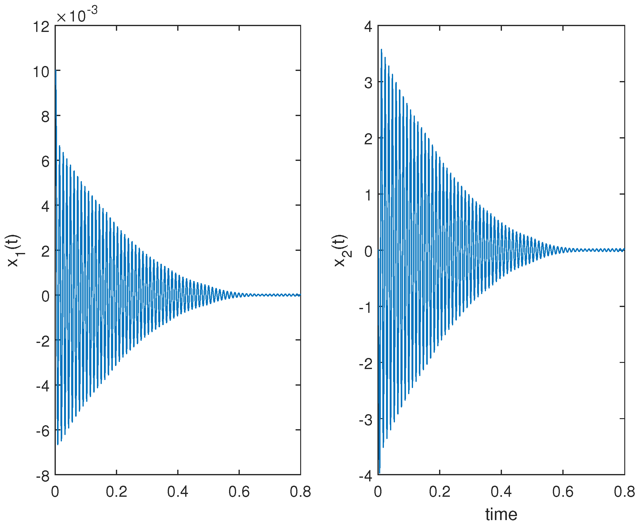
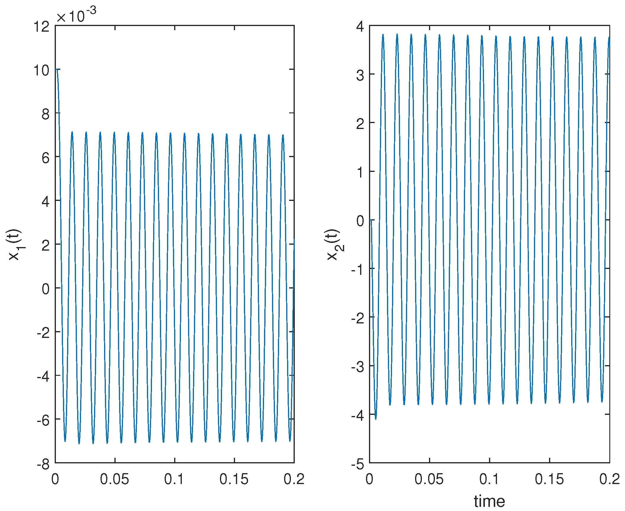
The state trajectories of the haptic system are shown in Figure 3 and Figure 4. From Table 1, the haptic system is stable for the case: $\alpha =0.131$ and $\beta =0.5$. Then, simulation studies are carried out considering the following four cases.

(1)

Case 1: $T=1$ ms, $t_d=1$ ms, $K=131,000$ N/m, $B=500$ Ns/m, $\alpha =0.131$, $\beta =0.500$.

(2)

Case 2: $T=1$ ms, $t_d=1$ ms, $K=137,890$ N/m, $B=500$ Ns/m, $\alpha =0.137$, $\beta =0.500$.

(3)

Case 3: $T=1$ ms, $t_d=1$ ms, $K=141,000$ N/m, $B=400$ Ns/m, $\alpha =0.141$, $\beta =0.400$.

(4)

Case 4: $T=1$ ms, $t_d=1$ ms, $K=143,985$ N/m, $B=400$ Ns/m, $\alpha =0.143$, $\beta =0.400$.

Figure 3 shows that the haptic system is stable when $\beta =0.5$ and $\alpha =0.131$, which proves the effectiveness of the proposed method. Figure 4 shows that the haptic system reaches critical stability when $\alpha =0.137$, and the theoretical value of $\alpha$ is $0.136$, which verifies the calculated accuracy of the proposed method. Similarly, the effectiveness of the proposed method is verified by Figure 5 that the haptic system is stable when $\beta =0.4$ and $\alpha =0.141$. Figure 6 also shows that the haptic system reaches critical stability when $\alpha =0.143$, which verifies the calculated accuracy of the proposed method.

5. Conclusions

In order to analyze the stability of haptic system with time delays, this paper has proposed a new delay-dependent stability criterion. By linearization, a haptic system model with time delays has been presented. An augmented LKF has been constructed, and an auxiliary function-based integral inequality has been introduced to estimate the derivative of the LKF. Therefore, a new stability criterion has been established to calculate the delay margins. Compared with existing methods, the advantages of this proposed criterion are mainly showed in two aspects. One aspect is that the proposed method provides a result, which is closer to the upper bound of the haptic system delay than other methods. The other is that, compared with other methods, the proposed method reduces the computational complexity to a greater extent. Finally, case studies have shown that both conservatism and computational complexity of the proposed method are reduced.

References

- Grajewski, D.; Górski, F.; Hamrol, A.; Zawadzki, P. Immersive and haptic educational simulations of assembly workplace conditions. Procedia Comput. Sci. 2015, 75, 359–368. [Google Scholar] [CrossRef] [Green Version]
- You, B.; Li, J.; Ding, L.; Xu, J.; Li, W.; Li, K.; Gao, H. Semi autonomous bilateral teleoperation of hexapod robot based on haptic force feedback. J. Intell. Robot. Syst. 2018, 91, 583–602. [Google Scholar] [CrossRef]
- Yoon, H.U.; Wang, R.F.; Hutchinson, S.A.; Hur, P. Customizing haptic and visual feedback for assistive human–robot interface and the effects on performance improvement. Robot. Auton. Syst. 2017, 91, 258–269. [Google Scholar] [CrossRef]
- Mashayekhi, A.; Behbahani, S.; Ficuciello, F.; Siciliano, B. Delay-dependent stability analysis in haptic rendering. J. Intell. Robot. Syst. 2019, 97, 33–45. [Google Scholar] [CrossRef]
- Shangguan, X.C.; He, Y.; Zhang, C.K.; Jin, L.; Yao, W.; Jiang, L.; Wu, M. Control performance standards-oriented event-triggered load frequency control for power systems under limited communication bandwidth. IEEE Trans. Control Syst. Technol. 2021. [Google Scholar] [CrossRef]
- Minsky, M.; Ming, O.; Steele, O.; Brooks, F.P.; Behensky, M. Feeling and seeing: Issues in force display. ACM SIGGRAPH Comput. Graph. 1990, 24, 235–241. [Google Scholar] [CrossRef]
- Hannaford, B.; Ryu, J.H. Time-domain passivity control of haptic interfaces. IEEE Trans. Robot. Autom. 1990, 18, 1–10. [Google Scholar] [CrossRef]
- Ryu, J.H.; Kim, Y.S.; Hannaford, B. Sampled- and continuous-time passivity and stability of virtual environments. IEEE Trans. Robot. 1990, 20, 772–776. [Google Scholar] [CrossRef]
- Gil, J.J.; Avello, A.; Rubio, Á.; Flórez, J. Stability analysis of a 1 DOF haptic interface using the Routh-Hurwitz criterion. IEEE Trans. Control Syst. Technol. 2004, 12, 583–588. [Google Scholar] [CrossRef]
- Gil, J.J.; Sánchez, E.; Hulin, T.; Preusche, C.; Hirzinger, G. Stability boundary for haptic rendering: Influence of damping and delay. J. Comput. Inf. Sci. Eng. 2009, 9, 011005. [Google Scholar] [CrossRef]
- Mashayekhi, A.; Behbahani, S.; Ficuciello, F.; Siciliano, B. Influence of human operator on stability of haptic rendering: A closed-form equation. Int. J. Intell. Robot. Appl. 2020, 4, 403–415. [Google Scholar] [CrossRef]
- He, Y.; Wang, Q.G.; Lin, C.; Wu, M. Augmented Lyapunov functional and delay dependent stability criteria for neutral systems. Int. J. Robust Nonlinear Control 2005, 15, 923933. [Google Scholar] [CrossRef]
- Ning, C.Y.; He, Y.; Wu, M.; Zhou, S.W. Indefinite derivative Lyapunov-Krasovskii functional method for input to state stability of nonlinear systems with time-delay. Appl. Math. Comput. 2015, 270, 534–542. [Google Scholar] [CrossRef]
- Zhang, C.K.; He, Y.; Jiang, L.; Wu, M. Notes on stability of time-delay systems: Bounding inequalities and augmented Lyapunov-Krasovskii functionals. IEEE Trans. Autom. Control 2017, 62, 5331–5336. [Google Scholar] [CrossRef] [Green Version]
- Wu, M.; He, Y.; She, J.H.; Liu, G.P. Delay-dependent criteria for robust stability of time-varying delay systems. Automatica 2004, 40, 1435–1439. [Google Scholar] [CrossRef]
- Seuret, A.; Gouaisbaut, F. Wirtinger-based integral inequality: Application to time-delay systems. Automatica 2013, 49, 2860–2866. [Google Scholar] [CrossRef] [Green Version]
- Park, P.; Lee, W.; Lee, S.Y. Auxiliary function-based integral inequalities for quadratic functions and their applications to time-delay systems. J. Frankl. Inst. 2015, 352, 1378–1396. [Google Scholar] [CrossRef]
- Zeng, H.B.; He, Y.; Wu, M.; She, J.H. Free-matrix-based integral inequality for stability analysis of systems with time-varying delay. IEEE Trans. Autom. Control 2015, 60, 2768–2772. [Google Scholar] [CrossRef]
- Zhang, C.K.; He, Y.; Jiang, L.; Wu, M.; Wang, Q.G. An extended reciprocally convex matrix inequality for stability analysis of systems with time-varying delay. Automatica 2017, 85, 481–485. [Google Scholar] [CrossRef]
- Kwon, W.; Koo, B.; Lee, S.M. Novel Lyapunov–Krasovskii functional with delay-dependent matrix for stability of time-varying delay systems. Appl. Math. Comput. 2018, 320, 149–157. [Google Scholar] [CrossRef]
- Zeng, H.B.; Liu, X.G.; Wang, W. A generalized free-matrix-based integral inequality for stability analysis of time-varying delay systems. Appl. Math. Comput. 2019, 354, 1–8. [Google Scholar] [CrossRef]
- Diolaiti, N.; Niemeyer, G.; Barbagli, F.; Salisbury, J.K. Stability of haptic rendering: Discretization, quantization, time delay, and coulomb effects. IEEE Trans. Robot. 2006, 22, 256–268. [Google Scholar] [CrossRef]
- Hulin, T.; Albu-Schaffer, A.; Hirzinger, G. Passivity and stability boundaries for haptic systems with time delay. IEEE Trans. Control Syst. Technol. 2014, 22, 1297–1309. [Google Scholar]
- Hogan, N. Controlling impedance at the man/machine interface. In Proceedings of the 1989 IEEE International Conference on Robotics and Automation, Scottsdale, AZ, USA, 14–19 May 1989; Volume 1, pp. 1626–1631. [Google Scholar]
- Zhang, C.K.; Long, F.; He, Y.; Yao, W.; Jiang, L.; Wu, M. A relaxed quadratic function negative-determination lemma and its application to time-delay systems. Automatica 2020, 113, 108764. [Google Scholar] [CrossRef]
Figure 1.
Structure diagram of a haptic device.