
Automatic Lane-Changing Decision Based on Single-Step Dynamic Game with Incomplete Information and Collision-Free Path Planning


1
School of Automotive and Transportation Engineering, Hefei University of Technology, Hefei 230009, China
2
Anhui Intelligent Vehicle Engineering Laboratory, Hefei 230009, China
3
School of Mechanical and Mechatronic Engineering, University of Technology, Sydney, NSW 2007, Australia
*
Authors to whom correspondence should be addressed.
Actuators 2021, 10(8), 173; https://0-doi-org.brum.beds.ac.uk/10.3390/act10080173
Submission received: 18 June 2021
/
Revised: 19 July 2021
/
Accepted: 22 July 2021
/
Published: 24 July 2021
(This article belongs to the Special Issue Actuators for Intelligent Electric Vehicles)
Abstract
:Traffic accidents are often caused by improper lane changes. Although the safety of lane-changing has attracted extensive attention in the vehicle and traffic fields, there are few studies considering the lateral comfort of vehicle users in lane-changing decision-making. Lane-changing decision-making by single-step dynamic game with incomplete information and path planning based on Bézier curve are proposed in this paper to coordinate vehicle lane-changing performance from safety payoff, velocity payoff, and comfort payoff. First, the lane-changing safety distance which is improved by collecting lane-changing data through simulated driving, and lane-changing time obtained by Bézier curve path planning are introduced into the game payoff, so that the selection of the lane-changing start time considers the vehicle safety, power performance and passenger comfort of the lane-changing process. Second, the lane-changing path without collision to the forward vehicle is obtained through the constrained Bézier curve, and the Bézier curve is further constrained to obtain a smoother lane-changing path. The path tracking sliding mode controller of front wheel angle compensation by radical basis function neural network is designed. Finally, the model in the loop simulation and the hardware in the loop experiment are carried out to verify the advantages of the proposed method. The results of three lane-changing conditions designed in the hardware in the loop experiment show that the vehicle safety, power performance, and passenger comfort of the vehicle controlled by the proposed method are better than that of human drivers in discretionary lane change and mandatory lane change scenarios.
1. Introduction
1.1. Background
With the increase in the number of vehicles, the fatality in traffic accidents keeps rising. According to a survey by the World Health Organization (WHO), approximately 1.24 million people were killed in road traffic accidents in 2010 [1]; this number has soared to 1.35 million in 2016 [2] and has remained stubbornly high in recent years. Furthermore, more than 90% of traffic accidents are caused by human error [3]. The drivers’ inaccurate estimation of traffic status or illegal operation under lane-changing conditions are the main factors of various traffic accidents [4,5]. Therefore, the safety of lane-changing has attracted extensive attention in the vehicle and traffic fields.
Vehicle lane-changing is a complex condition [6]. Successful lane-changing requires the driver to find an appropriate insertion position in the target lane, control the distance between the vehicle and the front vehicle, and maintain a safe driving position. The function of a lane-changing assistance system is to select an appropriate lane-changing time, plan a reasonable lane-changing path, and further coordinate the vehicle dynamic performance to realize lane-changing operation. The core of the control system includes three parts: early warning and decision-making, path planning, and path tracking. The analysis of the research status will be carried out from the above three aspects.
1.2. Literature Review and Analysis
A lane-changing early warning and decision-making system mainly determines when the vehicle changes its lane and directly affects the vehicle lane-changing safety. Dang et al. [7] realized the lane-changing warning function by vehicle-to-vehicle (V2V) communication. However, the maturity and popularization of V2V communication still need more time. Song et al. [8] used global positioning system and real-time kinematic (GPS-RTK) positioning technology to achieve high-precision vehicle positioning, which could be used to calculate the vehicles’ interval. Zhu et al. [9] classified and recognized drivers’ driving characteristics based on machine learning, and introduced the parameters considering drivers’ characteristics into the following vehicle safety distance to adjust lane-changing decision time. Nevertheless, a long time of data accumulation is needed to realize the recognition of driving characteristics. Butakov and Ioannou [10] collected a large amount of lane-changing related data to understand the reaction characteristics of drivers and vehicles in different driving environments before and during lane-changing, which provided a data basis for the relevant research. By comparing the relative distance between vehicles when drivers change lanes with the traditional headway safety distance, it can be found that the distance between the driver and front vehicle when drivers change the lanes may be less than the safety time distance. Because the distance between vehicles is often less than the safety distance in the real driving environment, the lane-changing decision based on vehicle interval is obviously not in line with the real scene. When there is a car behind the target lane, the lane-changing can be described as the game between the host car and the car behind the target lane. Yu et al. [11] introduced driver aggressiveness into game theory to design lane-changing decision-making to simulate human drivers. Meng et al. [12] combined receding horizon control into game theory and proved the effectiveness of the method through traffic case simulation. Cao et al. [13] established lane-level link performance function to evaluate the driving efficiency of the lane-changing behavior, to improve the macroscopic traffic flow efficiency.
In terms of path planning, there are two common methods, i.e., stochastic and kinematic methods [10]. Although the stochastic method can be used for dynamic planning according to the traffic environment, its planning results are difficult to accurately solve the physical parameters such as the expected yaw rate, which is not conducive to the design of the path tracking controller. The main methods based on kinematic are Polynomial curve [14,15], Clothoid curve [16], Bézier curve [17], and B-spline curve [18]. The kinematic method can describe the lane-changing path in the form of the equation which makes up for the defect of stochastic method, but it is difficult to constrain the path through the vehicle position relationship in the traffic environment. Bae et al. [19] designed a lane-changing path based on the quintic Bézier curve and compared it with the cubic Bézier curve. However, the constraints on the control points only consider the vehicle driving parameters of the starting point and the end point, and therefore there is a lack of basis for the selection of other constraint points. In addition, Mukai and Kawabe [20] used the multiparameter programming method to solve the problem of lane-changing decision and optimal path generation of model predictive control, but the scene construction was relatively simple and could not represent the real driving situation. Hu et al. [21] designed several cost functions to realize real-time path planning and optimal path selection, and the proposed method achieves real-time path planning and speed planning.
In the path tracking, the representative control methods are model predictive control, intelligent control, and sliding mode control. Falcone et al. [22] used the model predictive control to design an active steering path tracking controller. The LTV-MPC method achieved similar performance with nonlinear model predictive control at a lower hardware cost. Naranjo et al. [23] designed an overtaking system with path tracking and lane-changing functions using fuzzy controller. Ren et al. [24] designed the lane-changing path for the curve road and used the nonsingular terminal sliding mode controller to track the lane-changing path. Wu et al. [25] combined sliding mode control with active disturbance rejection control for path tracking, and compared with model predictive control, the effectiveness of the method was verified.
In the vehicle lane-changing system, the upper-level system’s decision on lane-changing instruction will have an impact on vehicle power performance and driving comfort when changing lane. Although Yu et al. [11], Meng et al. [12], and Cao et al. [13] verified that the designed decision-making method could improve the efficiency of macroscopic traffic flow, it lacked consideration of automobile power performance and driving comfort in the decision-making method. Liniger et al. [26] formulated three different racing games to study the game between automatic racing cars, which are of great value to promote the research of lane-changing games, and it was necessary to modify the focus of the payoff when applied to the passenger car system. In the aspect of path planning, the frequently used quintic polynomial path planning method [27] can easily obtain the yaw rate and lane-changing path. However, it can only adjust the lane-changing path by changing the whole process time, and therefore it is difficult to restrain the driving path through the distance relationship among the surrounding vehicles. The Bézier curve can be adjusted by constraint points, which is more flexible than the polynomial. Bulut et al. [28] compared the cubic Bézier curve with the quintic Bézier curve. The results showed that compared with the cubic Bézier curve, the variation of the quintic Bézier curve on velocity, lateral acceleration, longitudinal, and lateral jerk was more reasonable.
1.3. Paper Contribution and Organization
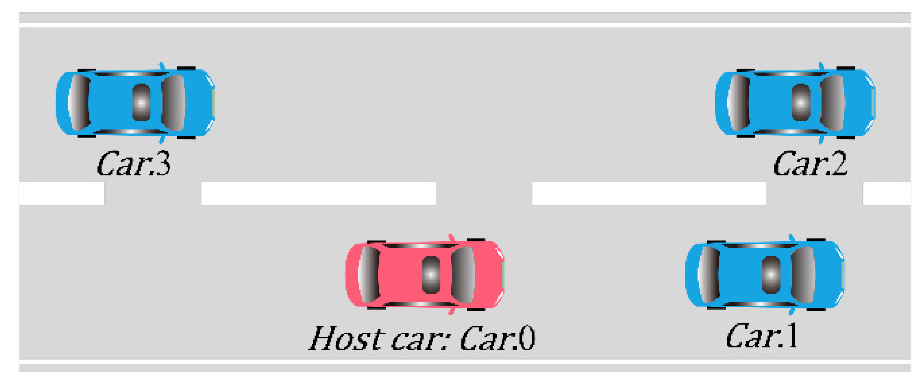
In order to improve the above shortcomings, the automatic lane-changing decision-making based on game theory with Bézier curve path planning is proposed. This paper has made the following contributions to the automatic vehicle lane-changing system. (I) In this paper, the existing safety distance model is improved, and the key parameters of the model are optimized through the lane-changing data of the human driver. (II) Through a single-step dynamic game with incomplete information, the safety payoff, comfort payoff, and velocity payoff are taken into account for the lane-changing system and achieve the balance in the optimization. (III) The lane-changing time calculated by the path planning layer is taken as an important parameter to ensure the safety and comfort of lane-changing, which realizes the strong coupling of decision layer and planning layer. The proposed algorithm can better adapt to both discretionary lane change (DLC) and mandatory lane change (MLC). This paper mainly studies the typical expressway driving environments as shown in Figure 1, in which Car.0 is the host car, Car.1 is the front car in the current lane, Car.2 is the front car in the target lane, and Car.3 is the rear car in the target lane.
The rest of this paper is organized as follows. In Section 2, the lane-changing safety distance is improved by collecting lane-changing data. In Section 3, the payoff function of the lane-changing decision-making method based on game theory is analyzed. In Section 4, the control points of the quintic Bézier curve are constrained to obtain the lane-changing path without forward collision. Based on the vehicle linear two-degree-of-freedom model, the path tracking sliding mode controller of front wheel angle compensation by radical basis function (RBF) neural network is designed. In Section 5, the model-in-the-loop (MIL) simulation, driving simulation test, and hardware-in-the-loop (HIL) verification are carried out. Section 6 is the discussion, and the conclusions are drawn in Section 7.
2. Lane-Changing Safety Distance
There are some driving parameters in the widely used Gipps car following model [29], which is difficult to obtain in the actual environment, so the headway safety distance model [30] is selected. The headway safety distance model is based on the time difference between the adjacent front and rear vehicles passing through the specified point in turn. When the relative speed of the two cars is small, there is an approximately linear relationship between the headway time and the distance of the two cars. Based on this, the following models are established:
where is the safety distance based on headway, is the headway time, generally 1.2–2.0 s, is the rear car speed, and is the safety margin, generally taken as 2–5 m [31].
Considering that the speed of the rear car often changes with the speed of the front car under the car-following condition, a safety distance margin is needed. When the braking distance model of the driver for emergency braking is applied to the car-following scenario, we get
where is the front car speed; is the braking distance; is the sum of driver reaction time and brake system coordination time, generally taken as 0.8–1.0 s; is the growth time of braking deceleration, generally taken as 0.1–0.2 s; and is the maximum braking deceleration that can be achieved during braking, generally taken as 6–8 m/s2.
It can be seen that the main influencing factor of the safety distance model based on the headway is the host car speed without considering the relative speed of adjacent vehicles. The braking distance model focuses on the relationship with the relative speed and is not sensitive to the speed of the host car. In order to make up for the shortcomings of the two models and achieve complementary advantages, the fusion safety distance (FSD) can be obtained as follows.:
where is the fusion of safety distance, is the weight coefficient of safety distance based on headway, and is the weight coefficient of braking distance model. When , the safety margin is used to replace the braking distance model.
Left lane-changing and right lane-changing often occur in the real driving process, and the steering characteristics of left lane-changing and right lane-changing are similar [32]. On the basis of the specific left lane-changing scene, the specific analyses of the safety distance between and other cars are carried out as follows.
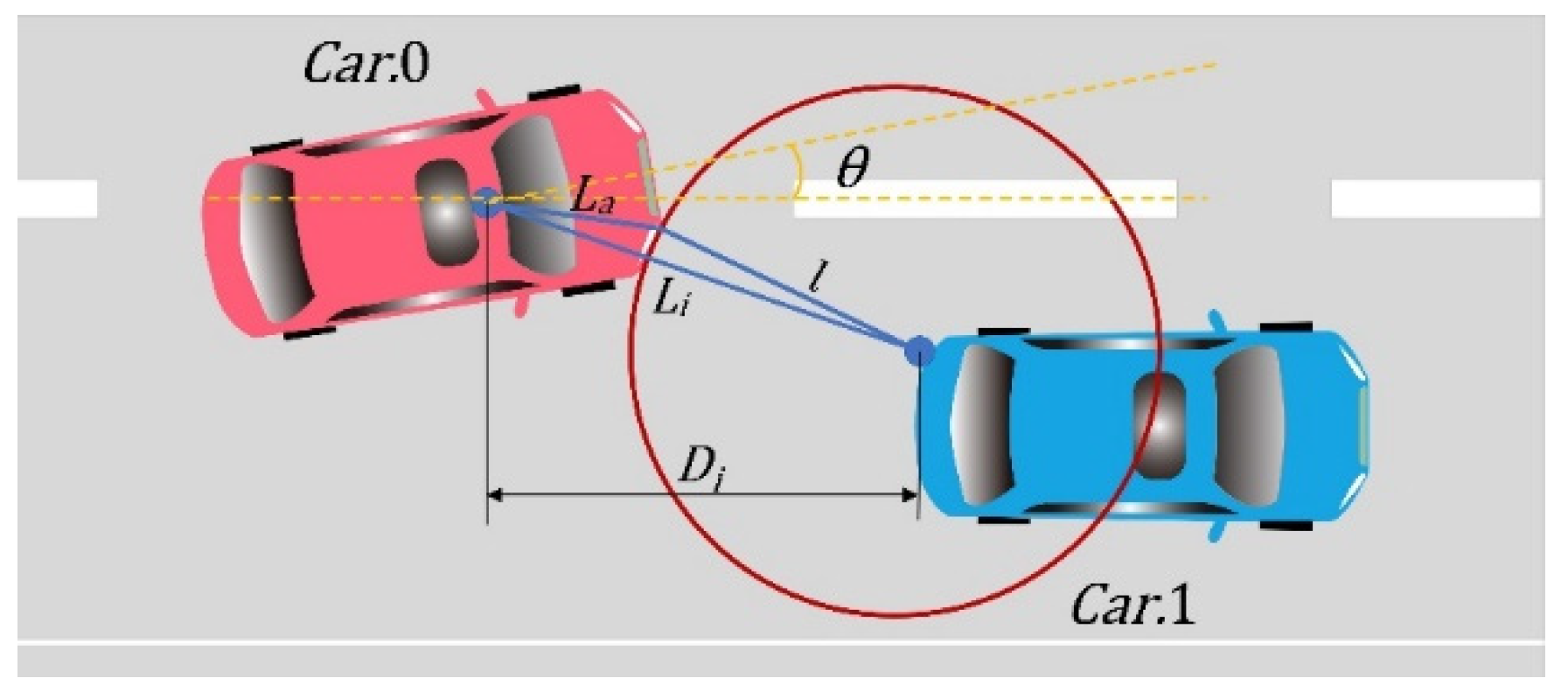
Based on (3), analyzing and may have a rear-end collision during the lane-changing process. It is necessary to consider the safety distance under emergency braking and lane changing, and the safety distance to avoid the rear-end collision is
where is the speed of , is the speed of , is the safety distance between and , is the time for to change its lanes, is the length of both car, is the width of both car, and is the ’s heading angle when it collides with . As is generally near the center line of the lane at this time, .
The collision between and occurs after the beginning of the lane-changing. Therefore, while ensuring the safety distance for the lane-changing, a safe car-following distance should be reserved for after entering the target lane to avoid subsequent rear-end collisions. According to the analysis of possible collisions based on the FSD, it can be concluded that the safety distance of to avoid rear-end collision or side scraping with as shown in (5), where is the FSD between and , and is the speed of .
The situation where collides with occurs at the end of lane-changing. At this time, has entered into the target lane, the steering wheel angle is about to return to zero, and the heading angle of is very small. Considering the above conditions, based on the FSD, the possible collision with is analyzed, and the safety distance to avoid the rear-end collision of can be expressed as (6), where the safety distance between and , and is the speed of .
Lane-changing habits of human driver is affected by age, gender, experience, etc. [33]. In order to ensure the authenticity of lane-changing related parameters in the model, 83 drivers with different driving experience and ages are specially invited for lane-changing operation on the driving simulator. Due to the difference between the subjective feeling of driving simulator and real vehicle, each driver is given a period of operation training.
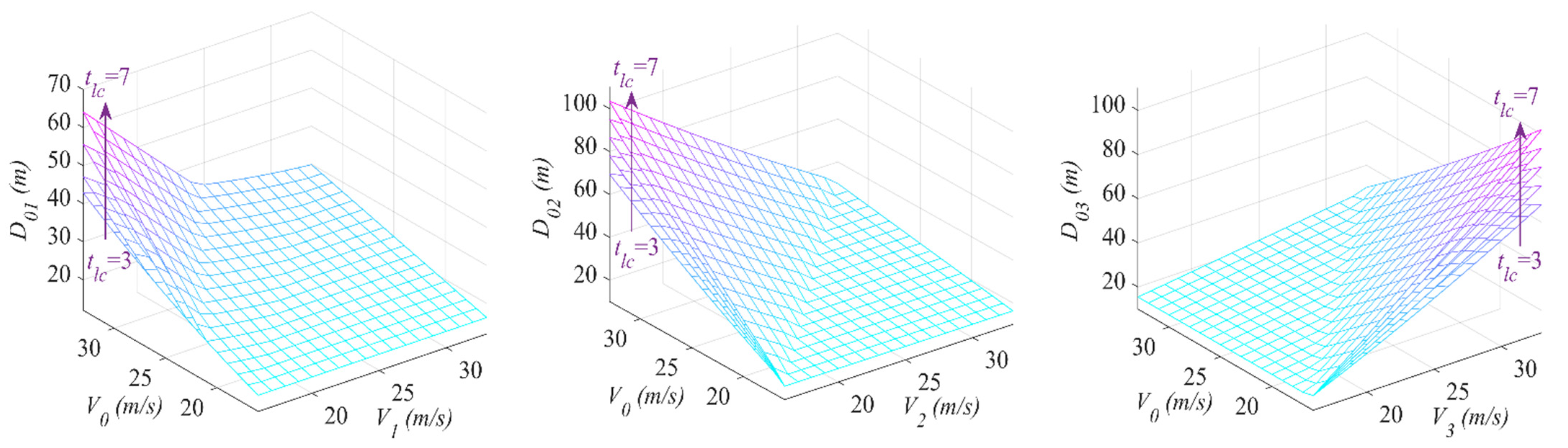
After completing the training, 83 drivers changed the lanes left and right for a total of 672 times. The final results are shown in Table 1, where is the average lane-changing time, is the standard deviation corresponding to , is the average maximum heading angle, and is the standard deviation corresponding to the . The last column in Table 1 is the total number of left and right lane-changing, and , , , , corresponding to the total lane-changing number. From Table 1, it can be concluded that the average value of the maximum heading angle is 3.20°, which indicates that the assumption that the maximum heading angle appears during lane-changing process is reasonable, and the average lane-changing time of 5.17 s is close to the 5.48 s [34]. The standard deviation corresponding to the lane-changing time and the maximum heading angle are small, which implies that the data are concentrated. According to the statistics of this lane-changing simulation data, 86.41% of the lane-changing time are in the interval (3.7, 6.3), so the change range of is taken as an integer of (3, 7), and the speed change range is set to 16~33 m/s. The changing rule of the lane-changing safety distance with is shown in Figure 2.
Through Figure 2, it can be found out that the greater the expected lane-changing time , the greater the lane-changing safety distance will be. Combining the data in Table 1, = 5.17 s is used to determine the lane-changing safety distance. The relevant parameters in the lane-changing safety distance model have been determined shown in Table 2.
3. Lane-Changing Decision-Making Based on Single-Step Dynamic Game with Incomplete Information
If refuses the lane-changing behavior of , it may cause a rear-end collision or side scraping. If accepts the lane-changing behavior of , will slow down and avoid . Therefore, there is a strong interaction between and in lane-changing scenarios. Game theory is a powerful tool to study the interaction between decision-makers [11]. The relationship between two cars can be regarded as players playing lane-changing games. Game behavior can be defined as a definite mathematical object which mainly includes three essential elements: player, strategy, and payoff [35]. First of all, in the process of driving, the strategies of both players will be adjusted according to the change of traffic environment, and the result of the game is determined once, so the game type between players belongs to single-step dynamic game. Second, assuming the relative distance and speed of the surrounding vehicles can be obtained by radar, but for vehicles without V2V communication function, only the controlled vehicle () can obtain the payoff function of both players in the game, that is, the information obtained by both players in the game is not complete. Finally, a single-step dynamic game with incomplete information is selected to model the game relationship between and in the lane-changing scene.
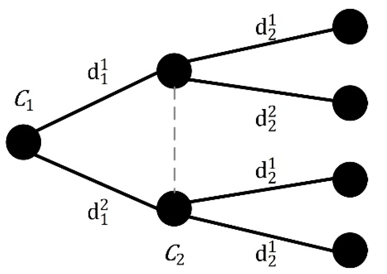
As shown in Figure 3, is the player, and is the corresponding strategy. When two players play a single-step dynamic game, the dotted line connects the two possible behaviors of which means that does not know what decision will make. This game is equivalent to and making a lane-changing decision at the same time, so that the extended game problem under incomplete information can be transformed into a static game problem for solution [36]. The pure strategies produced by this game can be written as shown in Table 3.
In Table 3, is lane-changing payoff of , is lane keeping payoff of , is the payoff of when accepts ’s lane-changing, and is the payoff of when refuses to change its lane.
3.1. Safety Payoff
Taking as the safety payoff, the safety payoff function can be described as
where , 0 is corresponding to , and 3 is corresponding to ; , 1 means lane-changing or accepting lane-changing, 2 means lane keeping or refusing lane-changing; , 02 represents the relationship between and , 01 represents the relationship between and , 03 represents the relationship between and , and 23 represents the relationship between and ; The numbers in , and play the role of codes, is the distance between vehicles, and is the lane-changing safety distance.
It can be seen that when , the safety payoff will directly reach , prompting to change its lane immediately. Similarly, when is close to , the payoff of will directly reach when it agrees changes the lane. When is close to , the lane-changing behavior of will not be carried out. If is close to , will change its lane immediately. Assuming that the speed of all vehicles is constant, when the above two situations occur at the same time, the collision loss caused by lane-changing or not is judged by combining other payoff functions.
3.2. Velocity Payoff
For both players of the game, the vehicle’s current speed of the player is set as the threshold that the player can continue to obtain, and the speed difference between the front vehicle and the player’s own vehicle is the payoff variable. According to this setting, the velocity payoff can be described as follows.
When there is a stationary car ahead or vehicle is detected currently on the ramp and needs to change its lane, the velocity payoff reaches the minimum value of −1. When the target speed is equal to the current speed, the velocity payoff is 0. Because the speed of each car on the road is basically within the speed limit range when driving at high speed, the velocity gain reaches 1 when the target speed is twice the current speed.
The significance of the velocity payoff setting is that when the speed of is greater than the current speed or the expected speed of , does not need to change its lanes. When the speed of is less than the current speed or the expected speed of , the speed of will be compared with the speed of . If the speed of can better meet the velocity payoff of , the lane-changing demand will be generated. That is to say, the earlier the lane-changing is completed, the better the vehicle power performance will be.
3.3. Comfort Payoff
When the speed of the preceding car is lower than the speed of the host car, the host car choosing to brake or change its lane to avoid the collision is needed. However, when the relative speed difference is large, the small lane-changing time is needed, the short lane-changing time will cause large lateral acceleration. Which is bad to the comfort of passengers. Therefore, connecting the lane changing time obtained from (14) and the comfort payoff. The comfort payoff is
where is half of the total lane-changing time shown in (14). The big speed difference between the preceding car and the host car will cause a small , and the time reserved for the driver to change the lanes is also very short. That is, the big lateral acceleration will be generated during lane-changing, leading to the worse comfort of passengers. The changing trend of is shown in Figure 4. It is indicated that when is more than 2.5 s, the change of is relatively gentle, while when is less than 2.5 s, the comfort payoff decreases sharply, which is consistent with the collected average lane-changing time of human drivers. The change trend of meets the influence rule of lane-changing time on lateral comfort.
3.4. Total Payoff and Game Solution
The total payoff is a linear combination of safety payoff, velocity payoff, and comfort payoff. , , and in (10) are the weights of corresponding payoff.
Excessive consideration of safety will reduce the lane-changing possibility, leading to system conservativeness increased. On the contrary, weakening the consideration of safety will increase the risk of collision [37]. This paper takes , , and .
The game model has at least one equilibrium point, which can be calculated by the change in the payoff function while driving. The problem of solving the equilibrium point is transformed into a problem of extreme points for solving, as in (11).
where and are the decisions of and , respectively; and are the strategy sets of the two cars; is the decision set of after the decision of ; is the decision under the decision set; and , are the final decisions of the two vehicles.
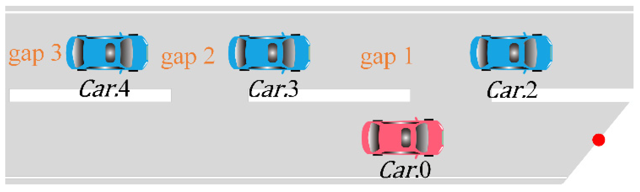
In order to verify the effectiveness of the proposed game method, the MLC scenario shown in Figure 5 designed in [11] is used for the simulation verification. Suppose the decision-making method used in that paper is , and the decision-making method used in this paper is . The comparison results are shown in Table 4. It can be seen from the Table 4 that the method of and adopt the same lane-changing cut-in position in the two scenarios of Test 1 and Test 2. In Test 3, the distance between and is only 10 m. At this time, still choosing to insert gap 2 will have a greater impact on the velocity payoff of , and it may even cause rear-end collision. Therefore, the proposed method chooses to change the lane immediately when overtakes . The price of delaying the lane-changing operation is to produce greater lateral acceleration, that is, to ensure driving safety by sacrificing part of the comfort. It is indicated that the proposed game lane-changing decision is effective.
4. Lane-Changing Path Planning and Tracking Control
The lane-changing path needs the lateral speed and lateral acceleration of the starting point and the ending point to be continuous, and the path can be constrained through the control points according to the traffic environment. The first part of this section will complete the lane-changing path planning by constraining the control points of the quintic Bézier curve. In the case of MLC, the high accuracy of the path tracking controller is required to control the vehicle interval accurately. There are some assumptions and simplifications in vehicle modeling, which will inevitably lead to the decline of tracking control accuracy [38]. Therefore, in the second part of this section, RBF neural network is used to compensate the vehicle front wheel angle modeling error under sliding mode control (SMC).
4.1. Lane-Changing Path Planning Based on Bézier Curve
The Bézier curve was invented by Pierre Bézier and has been widely used in computer graphics and animation [19]. Taking the lane direction as the coordinate X and the vertical lane direction as the coordinate Y, the lane change path can be given in the form of the parametric equation as
where and are the horizontal and vertical coordinates of the control point , respectively.
In order to meet the requirements of lane-changing lateral velocity and lateral acceleration at the starting and ending to be continuous, the lane width m, then ; .
Setting the lane-changing starting point , the vehicle-mounted radar is installed on the top of the vehicle. Considering that may collide to during the lane-changing process (shown in Figure 6), the horizontal coordinates and of the midpoint of the path are restricted shown in (13).
where is the time for to rear-end , is the longitudinal distance between the vehicle-mounted radar of and the closest point of , and is the linear distance between the vehicle-mounted radar and the closest point of . As is small, and , where is the distance from the vehicle-mounted radar to the front bumper of .
Then, for the vehicle to reach the lane-changing midpoint can be obtained as
Because , the control point has also been constrained. Setting that and are symmetrical about , so we get
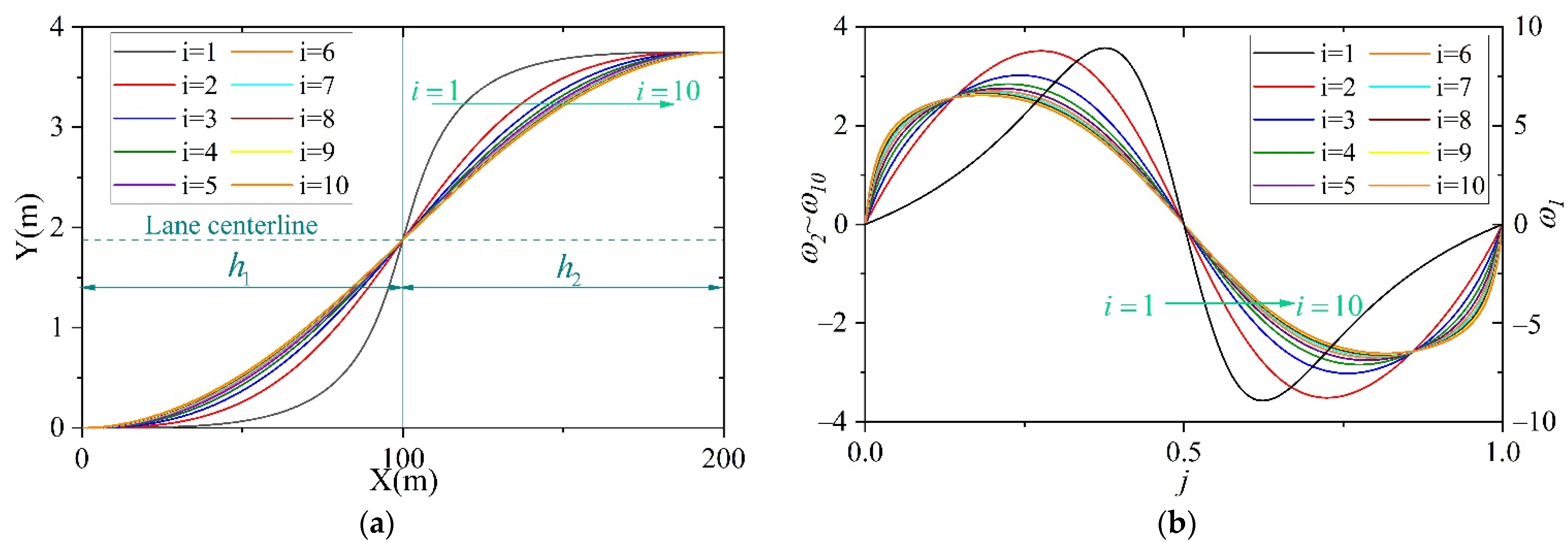
Take as an integer between [1,10] to draw Bézier curve shown in Figure 7a. It can be found out that when , , and no matter what the value of is, the curve will always pass , which also verifies the constraints setting of , , , and are correct and reasonable. In addition, the curve gradually tends to be flat with increasing. Therefore, it can be judged that with the increase of , the maximum yaw rate generated by the vehicle in the tracking process is decreased. In order to verify this conjecture, according to (16), the change trend of yaw rate corresponding to different values of is obtained shown in Figure 7b.
where is the curvature of the path and is the yaw rate; .
In Figure 7b, the maximum yaw rate that is generated by the planned path decreases with the increase of , which is conducive to providing better dynamism and comfort during the lane-changing process. However, with increases in , a greater rate of change in yaw will be generated near the starting and ending points of the lane-changing curve, which may cause passengers to become anxious when subjected to an instantaneously increasing lateral force. When , the decrease in yaw rate caused by the increase of is small, so is chosen to constrain and in this paper.
4.2. Path Tracking Controller
In the design of the path tracking controller, the following reasonable assumptions are put forward: (1) Ignore the roll, pitch, and vertical movement of the vehicle. (2) The vehicle lateral acceleration during the lane-changing is small, and the tires can be assumed working in the linear region. (3) The controller directly controls the front wheel angle. (4) The road surface is flat. Based on the above assumptions, the vehicle linear two-degree-of-freedom model built shown in (17).
where is the longitudinal velocity; is the lateral velocity; is the yaw rate; is the turning angle of the front wheels; is the mass of the vehicle; and are the cornering stiffnesses of the front and rear axles, respectively; and and are the distances from the center of mass to the front and rear axles, respectively.
There are some unavoidable disturbances during vehicle driving. In order to improve the robustness of the path tracking controller, the design of the sliding mode surface is
where , is the actual yaw angle of the vehicle, and is the desired yaw angle.
Differentiating (18) and combining with (17) and (19), we get
where ; ; ; is the desired yaw angle velocity; is the actual yaw angle acceleration.
In order to reduce the chattering of the path tracking system, the saturation function shown in (21) is used instead of the symbolic function.
Past research has shown that any nonlinear function over a compact set with arbitrary accuracy can be approximated by an RBF neural network [39], and the solution is hard to fall into the local optimal. Considering the inevitable error of the built model, the RBF neural network is used to compensate the front wheel angle by the sliding mode control. The input value of the RBF neural network is , and the performance index function of the RBF neural network is . The number of neurons in the hidden layer of the neural network is , and the output layer has one neuron. The Gaussian radial basis function of the hidden layer is
The compensation value of RBF neural network to the front wheel angle is obtained as follows:
where is the neural network weight vector, ; .
Then, the front wheel angle control law with the path tracking SMC compensated by RBF (SMC-RBF) is as follows:
In order to verify the effectiveness of the proposed tracking control method, the lane-changing path tracking results of SMC and SMC-RBF are compared in MIL simulation environment. The vehicle speed is 25 m/s, the total lane changing time is 5.1 s, and the simulation time is 10 s. The results are compared in Figure 8.
Figure 8a shows that although the sliding mode controller can complete path tracking without compensation by RBF, vehicle lateral error reaches 0.1524 m, which will have a greater impact in emergency lane changing scenes. In Figure 8b,c, the errors between the heading angle, the yaw rate and the reference values are reduced under RBF angle compensation. After the RBF is applied to compensate the angle, the accuracy of path tracking is greatly improved, and the maximum lateral error is only 0.0317 m. It shows that the designed path tracking sliding mode controller of front wheel angle compensation by RBF greatly improves the accuracy of path tracking.
5. Simulation and Result Analysis
In the Section 3, the effectiveness of the game lane-changing decision-making method is verified by simulation. In Section 4, the lane-changing curve is obtained by controlling the constraint points of Bézier curve, and SMC-RBF is used for path tracking. In this section, the advantages of the proposed method will be analyzed and discussed considerably by compared with the traditional method (decision-making by time to collision and quintic polynomial curve path planning) through MIL, and human driver through HIL.
5.1. MIL Simulation
In MIL simulation, a game decision-making method, a time-based decision-making method, Bézier curve path planning, and quintic polynomial path planning will be combined and applied to further prove the effectiveness of game lane-changing decision-making and Bézier curve path planning method (GT-B), and the influence of different decision-making methods and lane-changing paths on passenger comfort will be discussed. MIL simulation is carried out in Simulink/Carsim environment. Vehicle parameters are set in Carsim shown in Table 5.
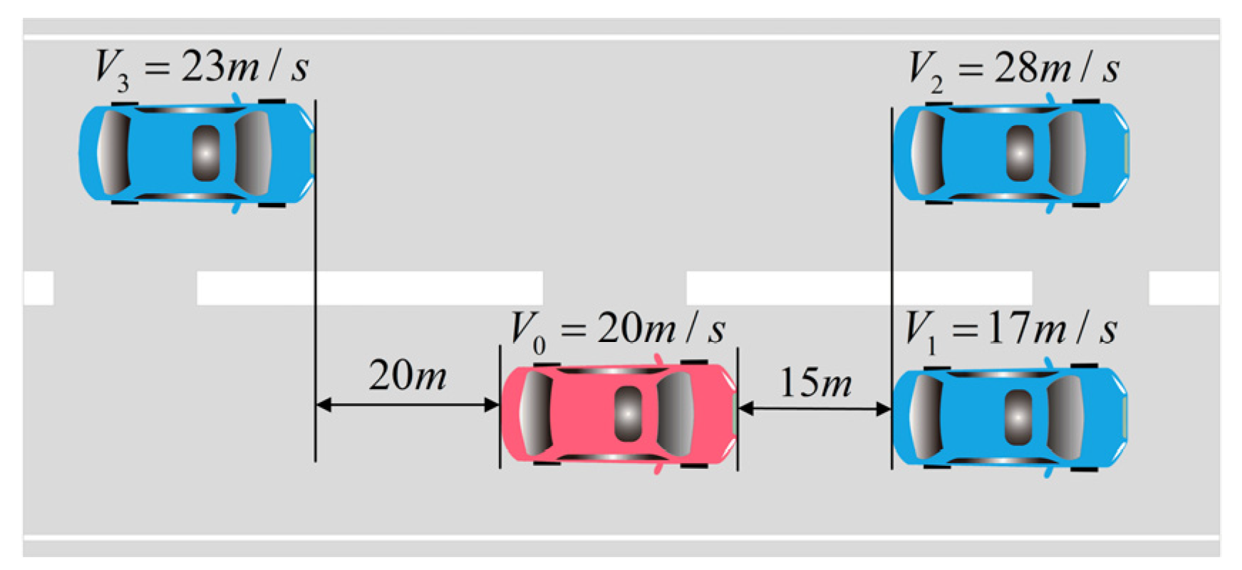
Build a traffic scene in Carsim (Figure 9), and perform a simulation with 15 s.
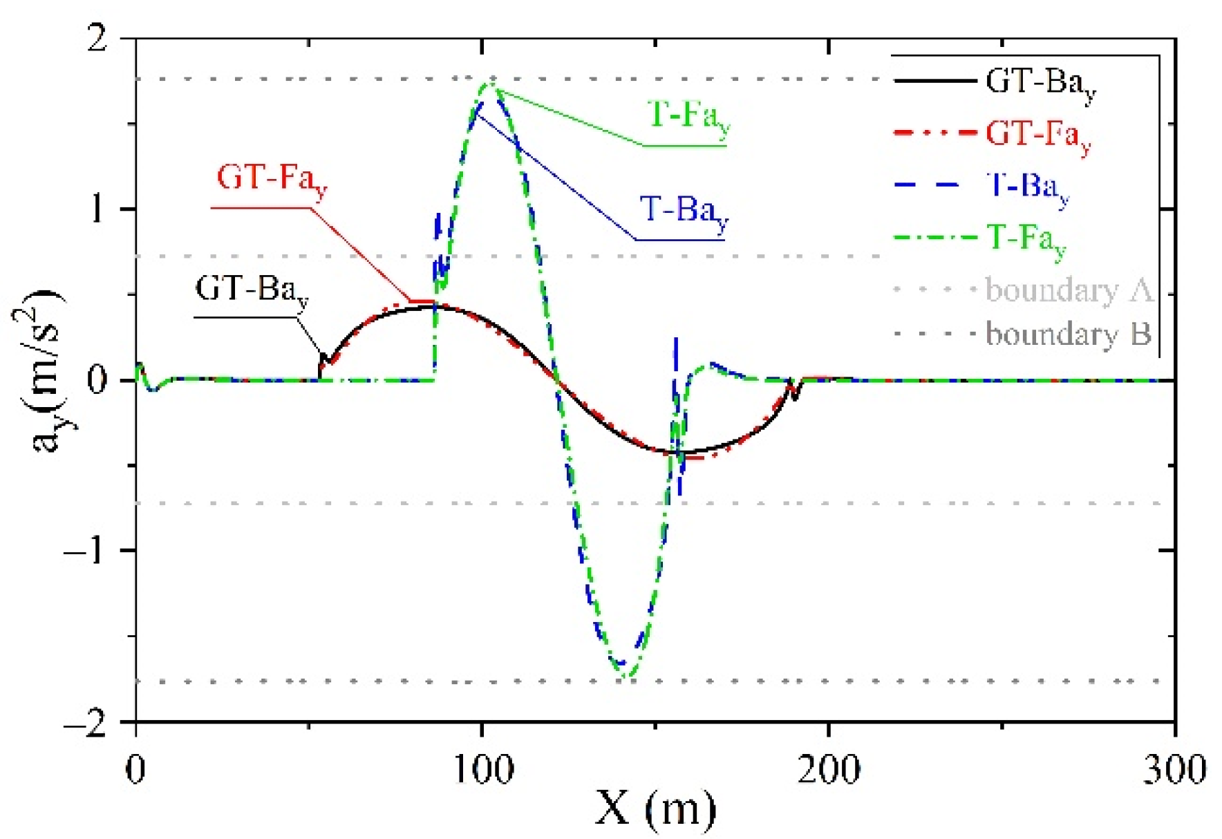
In Figure 10, GT-Bay is the lateral acceleration generated by tracking the Bézier curve under game decision-making; GT-Pay is the lateral acceleration generated by tracking the quintic polynomial curve under game decision-making; T-Bay is the lateral acceleration generated by tracking Bézier curve based on time to collision decision-making; T-Pay is the lateral acceleration generated by tracking the quintic polynomial curve based on the time to collision decision-making. The lateral acceleration division is shown in Table 6 where [40].
Compared with the lane-changing start time based on game theory and time to collision decision-making in Figure 10, it can be found out that by the decision-making method based on time to collision delays the lane-changing starting time is at 1.7 s. Owing to the close distance to at this time, the first half of the lane-changing has to be compressed to 1.8 s, making maximum lateral acceleration of reach 1.6595 m/s2. However, the vehicle by game decision-making starts to change its lane when the speed of is lower than , and the distance between and is large. As the lane-changing start time is earlier, the first half of lane change can be controlled to 3.4 s when the vehicle maximum lateral acceleration is only 0.4249 m/s2, reduced by 74.40%. Earlier lane-changing can also enable to reach the desired speed as soon as possible, so that improving the vehicle velocity payoff. Comparing GT-Pay with GT-Bay, it can be concluded that with the Bézier curve lane-changing path planning the maximum lateral acceleration is reduced by 8.03% than the quintic polynomial lane-changing path planning, and T-Bay also reduces 4.46% than T-Pay. The lane-changing path planned by the Bézier curve can provide higher passenger comfort. Compared with T-Pay, which is close to boundary B, the maximum lateral acceleration with GT-Bay is reduced by 75.54%, which greatly improves the passenger comfort.
5.2. HIL Experiment
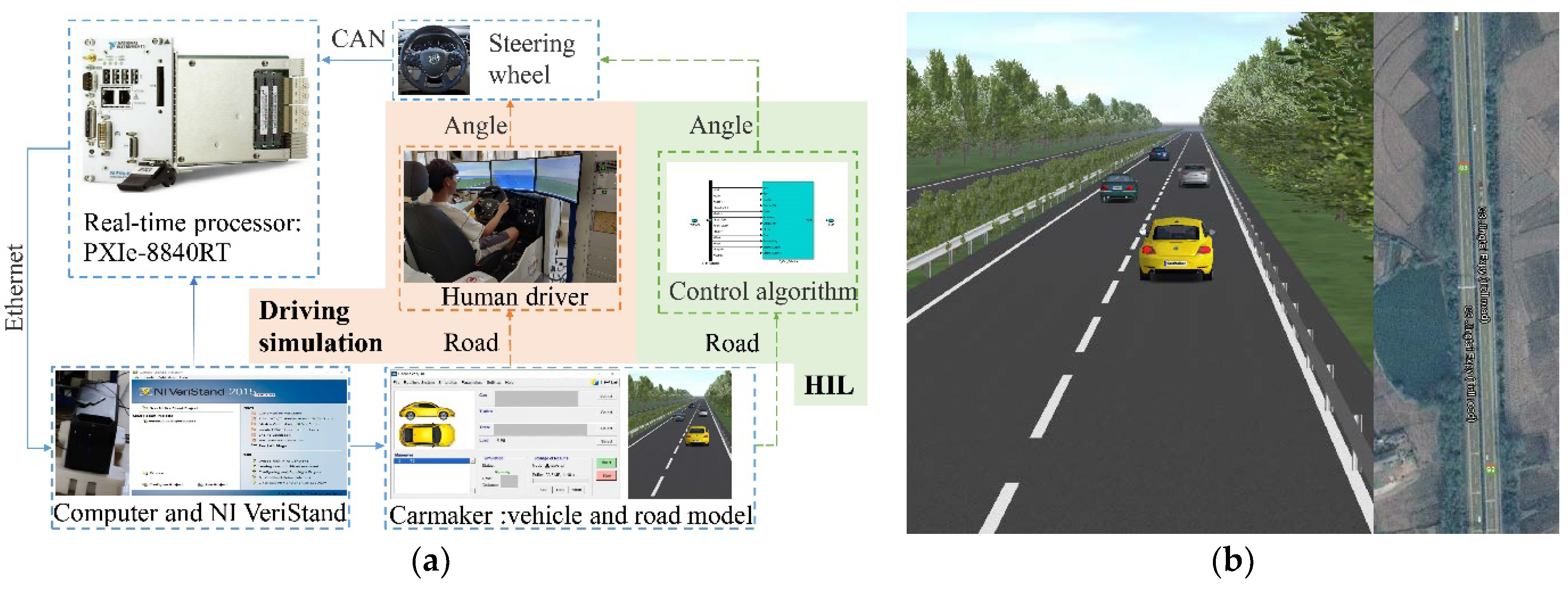
In order to analyze the difference of the decision-making and behavior differences between the proposed lane-changing method and the human driver, and to collect some lane-changing data of human drivers, it is necessary to invite drivers to conduct a real-car driving test in the same scene. However, due to the low safety, poor repeatability, and difficult scene modeling of real-car driving, it is decided to use driving simulator for HIL driving experiment. The principle of driving simulator is shown in Figure 11a. The core component of the system is the PXIe-8840RT real-time processor. NI VeriStand realizes the communication between the computer and PXI real-time processor through the network cable. The maximum simulation frequency in HIL experiment can reach 1000 Hz. In an HIL experiment, the steering wheel angle is controlled by the control program through the feedback information from Carmaker. In the driving experiment, the road and traffic scenes are displayed to the driver on the monitors, and the driver directly controls the steering wheel angle to realize the vehicle lateral movement.
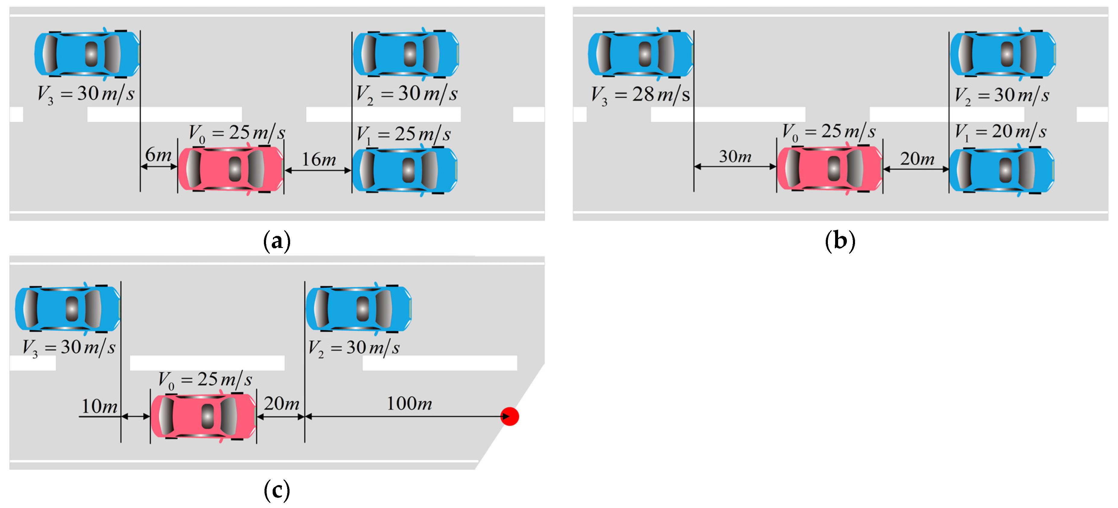
In the HIL experiment, in order to be close to the real road scene, the Hefei-Xuzhou Section of G3 Jingtai Expressway in China is simulated in Carmaker to build a one-way two-lane road with a total length of 700 m shown in Figure 11b. Three different traffic environments are set shown in Figure 12. From the setting of the relationship between the speed and distance of each vehicle, the software indicates that Case I represents a kind of condition without driving danger. If the driver wants to reach a higher speed, the lane needs to be changed timely; Case II represents an emergency driving situation, that is, the speed difference between the preceding car and the host car suddenly increases, and the driver can choose to lane-changing or brake for car-following. Case III is a common lane merging situation where the driver must perform lane-changing operations.
Five people are randomly selected from 83 people who perform the simulated lane-changing operations to conduct the driving tests in three scenarios. Before the simulated driving, the driver is only informed of the host car () speed and expected speed, and is not given any imply to the driver’s operation. To facilitate the description of the simulation results, the method proposed in this paper is referred to as GT-B in short. The code names of the driving experiments in the three cases are A, B, C, D, and E, which do not represent a specific driver. In order to simulate the speed fluctuation of the real high-speed vehicle during stable driving and the detection error of the radar equipment, the speed of the vehicle in the experiment is fluctuates in a sine curve with a fluctuation range of ±1 km/h, and cannot detect this small range of the speed fluctuations. That is to say, the speed obtained in the lane-changing game decision-making is not accurate.
5.2.1. Case I
In Case I, the target speed of is set as 33 m/s; at 2 s after the start of the simulation, surpasses to become the new , and surpasses at 6 s. The relationship between decision time and vehicle distances of different drivers under Case I is shown in Table 7, where is the shortest distance between and when crosses the lane, and is the shortest distance between and when crosses the lane. In order to express the process of surpassing more visually, take the distance between vehicles calculated in Figure 13a as the relative distance among vehicle-mounted radars, the relationship with the shortest distance among vehicles is . It can be seen from Figure 13a and Table 7 that the speed difference between and is large, chooses to follow up when has not completely surpassed under GT-B control. Further, a longer total lane-changing time is calculated by GT-B under the premise of ensuring a safety distance from the front vehicle, and the passenger comfort of is improved and the expected speed can be achieved earlier. Three drivers choose to follow up when does not completely surpass . This decision-making result is the same as GT-B. Driver C quickly follows and changes the lane when the speed of is judged to be high. Although the expected speed can be reached early, the driving safety of will decrease if the distance to the vehicle in front is closer. Before driver E starts to change lanes, is already greater than , indicating that lane change starting time of driver E is too conservative. The analysis shows that decision-making of GT-B is more in line with the human driver’s perception of the driving environment in Case I.
The vehicle path of driver B is compared with GT-B and shown in Figure 13b. The traffic setting in Case I is no risk of collision when lane is changed in the current scene, so GT-B chooses a longer lane-changing time, thus reducing the maximum lateral acceleration. In Figure 13b, the maximum lateral acceleration of the vehicle under the control of GT-B is only 0.32 m/s2, which is decreased by 36% than the maximum lateral acceleration of driver B of 0.5 m/s2 in the simulation, so that the comfort of passengers is improved.
5.2.2. Case II
Unlike Case I, the difference between and in Case II is relatively large. In order to achieve higher speed or maintain the current speed, the lane-changing is needed for . The expected speed of in Case II is set as 25 m/s. In Case II, two drivers choose to brake and follow , so there is no relevant comparison in Table 8. The remaining three drivers quickly judge the traffic situation after simulation beginning, and then all decisively change their lanes. Driver A makes full use of the distance with , and compared with driver B whose lane changing beginning time is close to driver A, the lateral acceleration of driver A during lane-changing is greatly reduced. However, generated by driver A and B is less than the safety distance margin, and a certain safety hazard has existed.
Figure 14a indicates that starts to slow down gradually after starts to change its lanes to guarantee a safety distance between different cars. Under the same deceleration with braking, the different lane-changing starting time of each driver leads to final different car-following distances of . In the same way, if the car-following distance is kept constant and the lane-changing starts later, requires greater deceleration with braking. Therefore, starting lane-changing operation early has smaller impact on other vehicles in traffic environment built in Case II.
The lane-changing time of driver C is close to the lane-changing time under GT-B control, so driver C and GT-B are selected for comparison shown in Figure 14. It can be seen that at the lane-changing midpoint, the distance between under the control of GT-B and is relatively close. Although there is no collision, it may have negative impact on the psychology of the passengers in . Table 8 shows that the time from beginning to midpoint is less than the time from midpoint to finish by human drivers, and human drivers may be more accustomed to cutting into the target lane and then overtaking, rather than overtaking during lane-changing. However, under dangerous situations, overtaking during lane-changing is obviously a benefit choice for both vehicle safety and passenger comfort. Figure 14b shows that the lateral acceleration of the vehicle driven by driver C has exceeded boundary B and reached 2.1240 m/s2. Under the control of GT-B, the lateral acceleration of during lane-changing is still within boundary A, and its maximum value is only 0.6055 m/s2, which is decreased by 71.49% than that by driver C.
5.2.3. Case III
Vehicle lane-changing conditions can be divided into (1) MLC due to environmental constraints and (2) DLC to improve driving environment [41]. In Case III, the vehicle is driving to a road condition that needs to be merged, such as driving into an underpass or driving into a main road from a ramp, so the scene of Case III can be regarded as MLC.
Because in Case III, and the distance between and is small, can not quickly change its lanes. Therefore, can only choose lane-changing after overtakes and become the new . In the first test of driving experiment, all five participants collide with or the end of the road due to the emergency of Case III. As a result of the emergency of MLC, it will increase the mental load of drivers [42]. Therefore, under the suggestions and requirements of the participants, each participant is given three opportunities to adapt to Case III, and the final data is obtained from the third test results. Even so, there is still a driver who collides with during the lane-changing. The lane-changing time and vehicle distance of the remaining four drivers and GT-B control are shown in Table 9.
Table 9 shows that no matter when the driver starts to change the lanes, their crossing time is basically the same as that of vehicles under GT-B control. However, generated by driver C and driver D is only 1.5 m. Although the road space is fully utilized, this lane-changing has certain risk. Only generated by driver A and GT-B is more reasonable. Judging from the lane-changing end time, the end time by GT-B is close to driver B and driver C, so they can reach the expected speed ahead of time compared with other experimental participants.
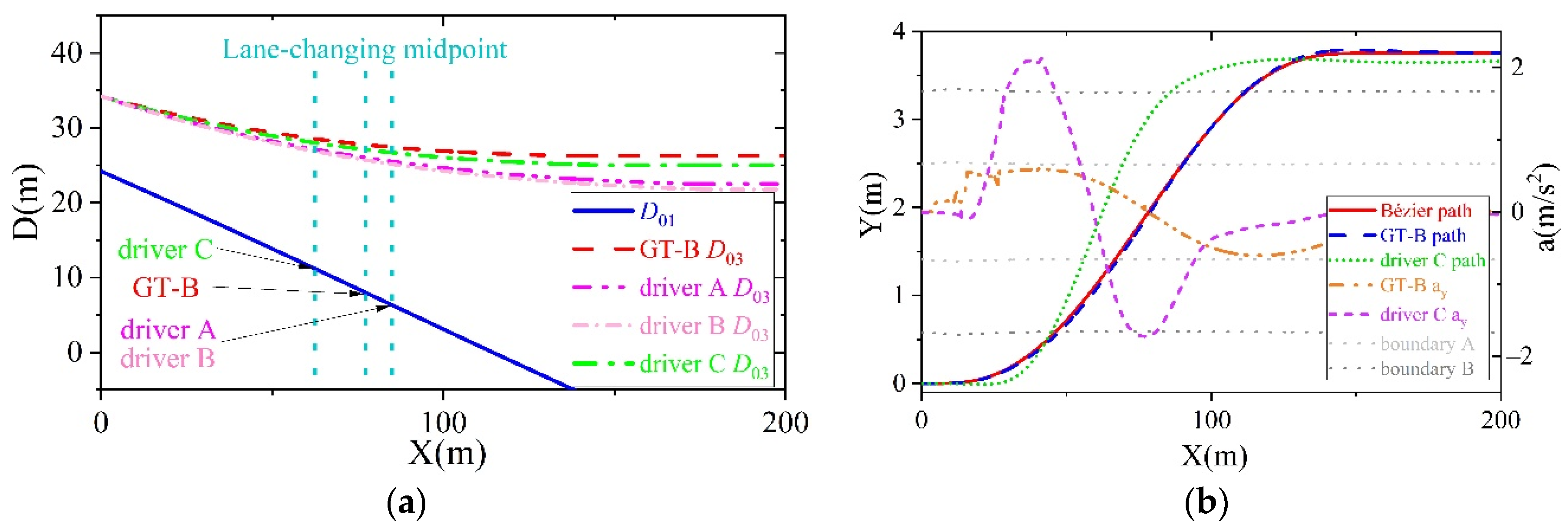
It can be determined from Table 9 and Figure 15a that as the front lane is about to end, vehicle safety, power performance, and human comfort can be coordinated by GT-B, so that drives to the adjacent lane with 6.5 m away from the end of the lane. Driver C with the same lane-changing start time is selected for comparison with GT-B shown in Figure 15b. Although the vehicle lateral acceleration under the control of GT-B is at the edge of boundary B, the lateral acceleration of vehicle driven by driver C already exceeds boundary C. In addition, the shorter lane-changing time will lead to the larger heading angle while crossing the lane. During turning the steering wheel to right after reaching the target lane, the maximum lateral acceleration of 2.9676 m/s2 is generated by driver C, and the maximum vehicle lateral acceleration under the control of GT-B is 1.8156 m/s2, which is 38.82% lower than that of driver C. The lateral deviation distance of the vehicle relative to the target lane center line by driver C reaches 0.375 m, and the close distance with the left guardrail will aggravate the deviation of the vehicle owing to the wind pressure in the case of high-speed driving, resulting in difficulty of the vehicle direction control. The maximum deviation distance of the vehicle relative to the lane centerline by SMC-RBF during the lane-changing is 0.125 m, and the vehicle can quickly return to the lane center.
6. Discussion
Comparing the analysis of lane-changing process under the control of GT-B with that of human drivers, it is obvious that vehicle safety, power performance, and human comfort can be coordinated well by the GT-B method. In the common traffic situation (Case I), part of vehicle power performance is sacrificed to guarantee driving safety, and the lane-changing time is appropriately extended to obtain good human comfort. In emergency situation (Case II), the vehicle’s performance is improved while guaranteeing its safety. In a very emergency situation (Case III), part of the power performance and human comfort are both sacrificed to make driving safety guaranteed. Moreover, vehicle performance by GT-B method is superior to that by human drivers in lane-changing path planning and vehicle lateral control. From the experiment results, it can be seen that GT-B method can balance the payoffs generated by lane-changing, and obtain more rapid, smoother, and safer lane-changing.
In order to simplify the lane-changing model, this paper makes some reasonable assumptions, such as the speed changing in a small range and only considering lane-changing in straight road. However, there are two conditions that may be needed to be noticed: (I) When the surrounding vehicles decelerate or accelerate suddenly, the lane-changing decision and the longitudinal motion of the host car will be affected. (II) Although lane-changing in a curved road is not recommended, it is still necessary to design an automatic lane-changing system that is safe for curved roads. When the vehicle is driving in the curved road to avoid the obstacle, the appropriate decision results are very important to ensure the vehicle and passengers’ safety. In the follow-up related research, the decision-making and path planning method will be studied and optimized based on the lane-changing in the curved road and consider longitudinal acceleration of each car in the traffic flow. Herrmann et al. [43] optimized the velocity on the available paths for the racing cars, which inspired velocity planning of host car in future study. The difference is that the racing cars need to fully utilize the maximum possible tire forces, whereas the passenger cars need to consider the impact of speed planning on ride comfort.
At present, the system is in the principle verification stage, so the vehicle distance signal obtained in the simulation is accurate value, however any distance measurement method has the error and noise. Vehicle state variables also need to be acquired through sensors, and sensor signals are bound to have delays and noises. If the system designed in this paper is to be applied to the actual vehicle in the future, it is necessary to study the sensor signal fusion technology and the vehicle state parameter estimation system. Although it is difficult to apply this method in the actual driving scene at present, the experimental data presented in this paper would promote the development of autonomous lane-changing systems and the further research based on this paper will help to reduce the number of traffic accidents caused by lane-changing.
7. Conclusions
A game of lane-changing decision-making with Bézier curve path planning is proposed in this paper which considers driving safety, power performance, and passenger comfort comprehensively. Lane-changing safety distance is obtained by using 83 driver lane-changing data. The lane-changing safety distance and lane-changing time calculated by the path planning layer are considered in game payoff to enhance safety considerations, which realizes the strong coupling between path planning layer and decision layer. The results of the planning layer are returned to the decision layer as the input, which can improve the security of the decision results. In addition, a detailed constrained optimization method is proposed for Bézier curves, which improves the safety, traceability, and comfort of the planned path. In the MIL simulation, it is proved that the method proposed in this paper greatly improves the vehicle safety and passenger comfort. The HIL experimental results indicate that the method proposed in this paper is superior to human drivers in the selection of lane change time, the control of vehicle interval, and can achieve the balance among vehicle safety, power performance and passenger comfort. In the HIL verification, there are not many driving scenarios, but the three lane-changing scenarios are representative that can be used for comparative tests.
It is obvious that the method proposed in this paper can meet the requirements well in the decision-making of lane-changing starting time, the total lane-changing time, the lane-changing planning path, and the tracking control of planned path in both scenarios of DLC and MLC. The results of this paper will accumulate experience for the further research.
Author Contributions
Conceptualization, H.W. and S.X.; methodology, H.W. and S.X.; software, S.X.; validation, S.X.; formal analysis, H.W., S.X. and L.D.; investigation, S.X.; resources, H.W.; data curation, S.X.; writing—original draft preparation, H.W. and S.X.; writing—review and editing, H.W. and S.X.; visualization, S.X. and L.D.; supervision, H.W. All authors have read and agreed to the published version of the manuscript.
Funding
This research was funded by National Nature Science Foundation of China, grant number U1564201, and Science Fund of Anhui Intelligent Vehicle Engineering Laboratory, grant number PA2018AFGS0026.
Data Availability Statement
The data presented in this study are available on request from the corresponding author. The data are not publicly available due to privacy.
Conflicts of Interest
The authors declare no conflict of interest.
References
- World Health Organization. Global Status Report on Road Safety 2013; Injury Prevention: London, UK, March 2013; pp. 4–10. Available online: https://www.who.int/violence_injury_prevention/road_safety_status/2013/en/ (accessed on 14 March 2021).
- World Health Organization. Global Status Report on Road Safety 2018; Injury Prevention: London, UK, June 2018; pp. 4–7. Available online: https://www.who.int/publications/i/item/9789241565684 (accessed on 14 March 2021).
- Singh, S. Critical Reasons for Crashes Investigated in The National Motor Vehicle Crash Causation Survey; DOT HS 812 115; Nat. Highway Traffic Safety Admin.: Washington, DC, USA, 2015.
- Kim, J.; Kim, J.; Jang, G.J.; Lee, M. Fast learning method for convolutional neural networks using extreme learning ma-chine and its application to lane detection. Neural Netw. 2017, 87, 109–121. [Google Scholar] [CrossRef]
- Zhao, D.; Lam, H.; Peng, H.; Bao, S.; LeBlanc, D.J.; Nobukawa, K.; Pan, C.S. Accelerated Evaluation of Automated Vehi-cles Safety in Lane-Change Scenarios Based on Importance Sampling Techniques. IEEE Trans. Intell. Trans.-Portation Syst. 2016, 18, 595–607. [Google Scholar] [CrossRef] [Green Version]
- Ali, Y.; Haque, M.M.; Zheng, Z.; Washington, S.; Yildirimoglu, M. A hazard-based duration model to quantify the impact of connected driving environment on safety during mandatory lane-changing. Transp. Res. Part C Emerg. Technol. 2019, 106, 113–131. [Google Scholar] [CrossRef]
- Dang, R.; Ding, J.; Su, B.; Yao, Q.; Tian, Y.; Li, K. A lane change warning system based on V2V communication. In Proceedings of the 17th International IEEE Conference on Intelligent Transportation Systems (ITSC), Qingdao, China, 8–11 October 2014; pp. 1923–1928. [Google Scholar]
- Song, Z.; Ji, J.; Zhang, R.; Cao, L. Development of a test equipment for rating front to rear-end collisions based on C-NCAP-2018. Int. J. Crashworthiness 2020, 1–11. [Google Scholar] [CrossRef]
- Zhu, B.; Yan, S.; Zhao, J.; Deng, W. Personalized Lane-Change Assistance System with Driver Behavior Identification. IEEE Trans. Veh. Technol. 2018, 67, 10293–10306. [Google Scholar] [CrossRef]
- Butakov, V.A.; Ioannou, P. Personalized Driver/Vehicle Lane Change Models for ADAS. IEEE Trans. Veh. Technol. 2015, 64, 4422–4431. [Google Scholar] [CrossRef]
- Yu, H.; Tseng, H.E.; Langari, R. A human-like game theory-based controller for automatic lane changing. Transp. Res. Part C Emerg. Technol. 2018, 88, 140–158. [Google Scholar] [CrossRef]
- Meng, F.; Su, J.; Liu, C.; Chen, W.-H. Dynamic decision making in lane change: Game theory with receding horizon. In Proceedings of the 2016 UKACC 11th International Conference on Control (CONTROL), Belfast, UK, 31 August–2 September 2016; pp. 1–6. [Google Scholar]
- Cao, P.; Xu, Z.; Fan, Q.; Liu, X. Analysing driving efficiency of mandatory lane change decision for autonomous vehicles. IET Intell. Transp. Syst. 2019, 13, 506–514. [Google Scholar] [CrossRef]
- Berglund, T.; Brodnik, A.; Jonsson, H.; Staffansson, M.; Soderkvist, I. Planning Smooth and Obstacle-Avoiding B-Spline Paths for Autonomous Mining Vehicles. IEEE Trans. Autom. Sci. Eng. 2009, 7, 167–172. [Google Scholar] [CrossRef]
- Stahl, T.; Wischnewski, A.; Betz, J.; Lienkamp, M. Multilayer Graph-Based Trajectory Planning for Race Vehicles in Dynamic Scenarios. In Proceedings of the 2019 IEEE Intelligent Transportation Systems Conference (ITSC), Paris, France, 9–12 June 2019. [Google Scholar]
- Broggi, A.; Medici, P.; Zani, P.; Coati, A.; Panciroli, M. Autonomous vehicles Control in the VisLab Intercontinental Au-tonomous Challenge. Annu. Rev. Control 2012, 36, 161–171. [Google Scholar] [CrossRef]
- Choi, J.-W.; Curry, R.; Elkaim, G. Path Planning Based on Bézier Curve for Autonomous Ground Vehicles. In Proceedings of the Advances in Electrical and Electronics Engineering—IAENG Special Edition of the World Congress on Engineering and Computer Science 2008, San Francisco, CA, USA, 22–24 October 2008; pp. 158–166. [Google Scholar] [CrossRef]
- Glaser, S.; Vanholme, B.; Mammar, S.; Gruyer, D.; Nouveliere, L. Maneuver-Based Trajectory Planning for Highly Autonomous Vehicles on Real Road With Traffic and Driver Interaction. IEEE Trans. Intell. Transp. Syst. 2010, 11, 589–606. [Google Scholar] [CrossRef]
- Bae, I.; Moon, J.; Park, H.; Kim, J.H.; Kim, S. Path generation and tracking based on a Bézier curve for a steering rate controller of autonomous vehicles. In Proceedings of the 16th International IEEE Conference on Intelligent Transportation Systems (ITSC 2013), Kurhaus, The Hague, 6–9 October 2013; pp. 436–441. [Google Scholar]
- Mukai, M.; Kawabe, T. Model predictive control for lane change decision assist system using hybrid system representation. In Proceedings of the 2006 SICE-ICASE International Joint Conference, Busan, Korea, 18–21 October 2006; pp. 5120–5125. [Google Scholar] [CrossRef]
- Hu, X.; Chen, L.; Tang, B.; Cao, D.; He, H. Dynamic path planning for autonomous driving on various roads with avoidance of static and moving obstacles. Mech. Syst. Signal Process. 2018, 100, 482–500. [Google Scholar] [CrossRef]
- Falcone, P.; Borrelli, F.; Asgari, J.; Tseng, H.E.; Hrovat, D. Predictive Active Steering Control for Autonomous Vehicle Systems. IEEE Trans. Control. Syst. Technol. 2007, 15, 566–580. [Google Scholar] [CrossRef]
- Naranjo, J.E.; Gonzalez, C.; Garcia, R.; De Pedro, T. Lane-Change Fuzzy Control in Autonomous Vehicles for the Overtaking Maneuver. IEEE Trans. Intell. Transp. Syst. 2008, 9, 438–450. [Google Scholar] [CrossRef] [Green Version]
- Ren, D.; Zhang, J.; Zhang, J.; Cui, S. Trajectory planning and yaw rate tracking control for lane changing of intelligent vehicle on curved road. Sci. China Ser. E Technol. Sci. 2011, 54, 630–642. [Google Scholar] [CrossRef]
- Wu, Y.; Wang, L.; Zhang, J.; Li, F. Path Following Control of Autonomous Ground Vehicle Based on Nonsingular Terminal Sliding Mode and Active Disturbance Rejection Control. IEEE Trans. Veh. Technol. 2019, 68, 6379–6390. [Google Scholar] [CrossRef]
- Liniger, A.; Lygeros, J. A Noncooperative Game Approach to Autonomous Racing. IEEE Trans. Control. Syst. Technol. 2019, 28, 884–897. [Google Scholar] [CrossRef] [Green Version]
- Yao, W.; Zhao, H.; Davoine, F.; Zha, H. Learning lane change trajectories from on-road driving data. In Proceedings of the 2012 IEEE Intelligent Vehicles Symposium, Madrid, Spain, 3–7 June 2012; pp. 885–890. [Google Scholar]
- Bulut, V. Path planning for autonomous ground vehicles based on quintic trigonometric Bézier curve. J. Braz. Soc. Mech. Sci. Eng. 2021, 43, 1–14. [Google Scholar] [CrossRef]
- Gipps, G. A behavioural car-following model for computer simulation. Transp. Res. Board 1981, 15, 105–111. [Google Scholar] [CrossRef]
- Aycin, M.F.; Benekohal, R.E. Linear Acceleration Car-Following Model Development and Validation. Transp. Res. Rec. J. Transp. Res. Board 1998, 1644, 10–19. [Google Scholar] [CrossRef]
- Seiler, P.; Song, B.; Hedrick, J.K. Development of a Collision Avoidance System. SAE Tech. Paper Ser. 1998, 98PC417. [Google Scholar] [CrossRef]
- Salvucci, D.D.; Liu, A. The time course of a lane change: Driver control and eye-movement behavior. Transp. Res. Part F Traffic Psychol. Behav. 2002, 5, 123–132. [Google Scholar] [CrossRef]
- Sharma, A.; Ali, Y.; Saifuzzaman, M.; Zheng, Z.; Haque, M. Human Factors in Modelling Mixed Traffic of Traditional, Connected, and Au-tomated Vehicles. Advances in Intelligent Systems and Computing; Springer: Berlin, Germany, 2017; pp. 262–273. [Google Scholar]
- Long, X.; Zhang, L.; Liu, S.; Wang, J. Research on Decision-Making Behavior of Discretionary Lane-Changing Based on Cumula-tive Prospect Theory. J. Adv. Transp. 2020, 2020, 1291342. [Google Scholar] [CrossRef]
- Nash, J. Non-Cooperative Games. Ann. Math. 1951, 54, 286–295. [Google Scholar] [CrossRef]
- Başar, T.; Olsder, G.J. Dynamic Noncooperative Game Theory, 2nd ed.; SIAM Publications: Philadelphia, PA, USA, 1998. [Google Scholar] [CrossRef]
- Lindgren, A.; Chen, F. State of the art analysis: An overview of advanced driver assistance systems (ADAS) and possible human factors issues. In Proceedings of the Human Factors and Economic Aspects on Safety, Linköping, Sweden, 5–7 April 2007; Volume 38, pp. 38–50. [Google Scholar]
- Zhang, K.; Cui, S.M.; Wang, J.F. Intelligent vehicle’s path tracking control based on self-adaptive RBF network compensation. Control Decision. 2014, 29, 627–631. [Google Scholar]
- Sonfack, L.L.; Kenné, G.; Fombu, A.M. An improved adaptive RBF neuro-sliding mode control strategy: Application to a static synchronous series compensator controlled system. Int. Trans. Electr. Energy Syst. 2019, 29, e2835. [Google Scholar] [CrossRef]
- Jr, N.H.S. An Investigation of Vehicle Critical Speed and its Influence on Lane-Change Trajectories. Ph.D. Thesis, University of Texas at Austin, Austin, TX, USA, 1997. [Google Scholar]
- Toledo, T.; Koutsopoulos, H.N.; Ben-Akiva, M.E. Modeling Integrated Lane-Changing Behavior. Transp. Res. Rec. J. Transp. Res. Board 2003, 1857, 30–38. [Google Scholar] [CrossRef] [Green Version]
- Plankermann, K. Human Factors as Causes for Road Traffic Accidents in the Sultanate of Oman Under Consideration of Road Construction Designs. Ph.D.’s Thesis, University of Regensburg, Regensburg, Germany, 2014. [Google Scholar] [CrossRef]
- Herrmann, T.; Wischnewski, A.; Hermansdorfer, L.; Betz, J.; Lienkamp, M. Real-Time Adaptive Velocity Optimization for Autonomous Electric Cars at the Limits of Handling. IEEE Trans. Intell. Veh. 2020. [Google Scholar] [CrossRef]
Figure 1.
Driving environment and vehicle code name.

Figure 2.
Variation of lane-changing safety distance with .

Figure 3.
The extended schematic diagram of single-step game.

Figure 4.
The change trend of .

Figure 5.
MLC scenario.

Figure 6.
The relationship between and avoiding collision.

Figure 7.
Influence of different values on lane-changing path. (a) Comparison of driving path. (b) Comparison of yaw rate.
Figure 7.
Influence of different values on lane-changing path. (a) Comparison of driving path. (b) Comparison of yaw rate.

Figure 8.
Comparison of path following controller with and without angle compensation control. (a) Comparison of driving path. (b) Comparison of heading angle. (c) Comparison of yaw rate.
Figure 8.
Comparison of path following controller with and without angle compensation control. (a) Comparison of driving path. (b) Comparison of heading angle. (c) Comparison of yaw rate.

Figure 9.
Traffic environment in MIL.

Figure 10.
Comparison of lateral acceleration under different combinations of decision-making and path planning methods.
Figure 10.
Comparison of lateral acceleration under different combinations of decision-making and path planning methods.

Figure 11.
Experimental equipment framework and road modeling. (a) Driving simulation and HIL implementation. (b) Hefei-Xuzhou Section of G3 Jingtai Expressway in China in Carmaker.
Figure 11.
Experimental equipment framework and road modeling. (a) Driving simulation and HIL implementation. (b) Hefei-Xuzhou Section of G3 Jingtai Expressway in China in Carmaker.

Figure 12.
HIL traffic environment settings. (a) Traffic environment Case I. (b) Traffic environment Case II. (c) Traffic environment Case III.
Figure 12.
HIL traffic environment settings. (a) Traffic environment Case I. (b) Traffic environment Case II. (c) Traffic environment Case III.

Figure 13.
Vehicles’ interval, vehicle path and lateral acceleration in Case I. (a) Decision-making time and distance. (b) Vehicle path and lateral acceleration.
Figure 13.
Vehicles’ interval, vehicle path and lateral acceleration in Case I. (a) Decision-making time and distance. (b) Vehicle path and lateral acceleration.

Figure 14.
Vehicles’ interval, path and lateral acceleration in Case II. (a) Vehicle interval during lane-changing by different drivers. (b) Vehicle path and lateral acceleration.
Figure 14.
Vehicles’ interval, path and lateral acceleration in Case II. (a) Vehicle interval during lane-changing by different drivers. (b) Vehicle path and lateral acceleration.

Figure 15.
Vehicles’ interval, path and lateral acceleration in Case III. (a) Relative distance between other vehicles and ; (b) Vehicle path and lateral acceleration.
Figure 15.
Vehicles’ interval, path and lateral acceleration in Case III. (a) Relative distance between other vehicles and ; (b) Vehicle path and lateral acceleration.


Table 1.
Results of driving simulation lane-changing experiment.
| Left Lane-Changing | Right Lane-Changing | General | |
|---|---|---|---|
| Number of times | 347 | 325 | 672 |
| 5.11 | 5.23 | 5.17 | |
| 0.8002 | 0.9403 | 0.8703 | |
| (deg) | 3.33 | 3.10 | 3.20 |
| 0.6410 | 0.6122 | 0.6266 |
Table 2.
Parameters of lane-changing safety distance model.
| Parameter | Value | Unit |
|---|---|---|
| 4.2 | m | |
| 1.8 | m | |
| 3 | m | |
| 3.20 | deg | |
| 5.17 | ||
| 1.2 | s | |
| 0.15 | s | |
| 0.9 | s | |
| 0.65 | - | |
| 0.35 | - | |
| 7 | m/s2 |
Table 3.
Pure strategies of the lane-changing game.
| Player | ||
|---|---|---|
| Lane-Changing/Accept | Lane Keeping/Refuse | |
Table 4.
Lane-changing cut-in positions comparison.
| Test 1 | Test 2 | Test 3 | ||
|---|---|---|---|---|
| Parameter | (m/s2) | 10 | 10 | 10 |
| (m) | 50 | 50 | 50 | |
| (m) | 10 | 10 | 10 | |
| (m/s2) | 15 | 15 | 15 | |
| (m) | −20 | −8 | −8 | |
| (m/s2) | 15 | 15 | 15 | |
| (m) | −30 | −25 | −18 | |
| (m/s2) | 15 | 15 | 15 | |
| Decision | gap 1 | gap 2 | gap 2 | |
| gap 1 | gap 2 | gap 3 | ||
Table 5.
Parameters of simulation vehicle.
| Parameter | Value | Units |
|---|---|---|
| Distance from the center of mass to the front axis, | 1.232 | m |
| Distance from the center of mass to the rear axis, | 1.468 | m |
| Vehicle mass, | 1520 | kg |
| Total lateral stiffness of front axle, | 66,900 | N/rad |
| Total lateral stiffness of rear axle, | 62,700 | N/rad |
| The moment of inertia, | 3965 | kg·m2 |
Table 6.
Classification of lateral acceleration intensity.
| Level | Lateral Acceleration Range (m/s2) | Code Name |
|---|---|---|
| Normal-level | boundary A | |
| Strong-level | boundary B | |
| Restricted-level | boundary C | |
| Maximum-level | boundary D |
Table 7.
Driving parameters of different drivers under Case I.
| Driver | Begin Time (s) | Finish Time (s) | ||
|---|---|---|---|---|
| A | 5.4 | 10.3 | 11.5 | 13.5 |
| B | 5.9 | 11.7 | 13.9 | 14.4 |
| C | 4.3 | 13.2 | 6.3 | 14.8 |
| D | 6.7 | 13.4 | 17.9 | 14.4 |
| E | 11.5 | 19.9 | 45.0 | 17.5 |
| GT-B | 5.3 | 13.3 | 11.0 | 13.5 |
Table 8.
Driving parameters of different drivers under Case II.
| Driver | Begin Time (s) | Midpoint Time (s) | Finish Time (s) | ||
|---|---|---|---|---|---|
| A | 1.3 | 3.4 | 6.2 | 2.3 | 1.4571 |
| B | 1.5 | 3.4 | 5.4 | 2.3 | 2.1989 |
| C | 0.6 | 2.5 | 5.9 | 7.2 | 2.1240 |
| GT-B | 0.2 | 3.1 | 6.1 | 4.0 | 0.6031 |
Table 9.
Driving parameters of different drivers under Case III.
| Driver | Begin Time (s) | Midpoint Time (s) | Finish Time (s) | ||
|---|---|---|---|---|---|
| A | 1.7 | 3.7 | 5.8 | 6.5 | 3.4 |
| B | 1.5 | 3.8 | 5.3 | 4 | 3.8 |
| C | 2.0 | 3.9 | 5.5 | 1.5 | 4.3 |
| D | 2.5 | 3.9 | 7.0 | 1.5 | 4.3 |
| GT-B | 2.0 | 3.7 | 5.4 | 6.5 | 3.4 |
Publisher’s Note: MDPI stays neutral with regard to jurisdictional claims in published maps and institutional affiliations. |
© 2021 by the authors. Licensee MDPI, Basel, Switzerland. This article is an open access article distributed under the terms and conditions of the Creative Commons Attribution (CC BY) license (https://creativecommons.org/licenses/by/4.0/).
Share and Cite
MDPI and ACS Style
Wang, H.; Xu, S.; Deng, L. Automatic Lane-Changing Decision Based on Single-Step Dynamic Game with Incomplete Information and Collision-Free Path Planning. Actuators 2021, 10, 173. https://0-doi-org.brum.beds.ac.uk/10.3390/act10080173
AMA Style
Wang H, Xu S, Deng L. Automatic Lane-Changing Decision Based on Single-Step Dynamic Game with Incomplete Information and Collision-Free Path Planning. Actuators. 2021; 10(8):173. https://0-doi-org.brum.beds.ac.uk/10.3390/act10080173
Chicago/Turabian StyleWang, Hongbo, Shihan Xu, and Longze Deng. 2021. "Automatic Lane-Changing Decision Based on Single-Step Dynamic Game with Incomplete Information and Collision-Free Path Planning" Actuators 10, no. 8: 173. https://0-doi-org.brum.beds.ac.uk/10.3390/act10080173
Note that from the first issue of 2016, this journal uses article numbers instead of page numbers. See further details here.