Segment Drift Control with a Supervision Mechanism for Autonomous Vehicles

Abstract

Stable maneuverability is extremely important for the overall safety and robustness of autonomous vehicles under extreme conditions, and automated drift is able to ensure the widest possible range of maneuverability. However, due to the strong nonlinearity and fast vehicle dynamics occurring during the drift process, drift control is challenging. In view of the drift parking scenario, this paper proposes a segmented drift parking method to improve the handling ability of vehicles under extreme conditions. The whole process is divided into two parts: the location approach part and the drift part. The model predictive control (MPC) method was used in the approach to achieve consistency between the actual state and the expected state. For drift, the open-loop control law was designed on the basis of drift trajectories obtained by professional drivers. The drift monitoring strategy aims to monitor the whole drift process and improve the success rate of the drift. A simulation and an actual vehicle test platform were built, and the test results show that the proposed algorithm can be used to achieve accurate vehicle drift to the parking position.

1. Introduction

The stability of the vehicle chassis has always been a matter of concern. Chassis design can be divided into different classifications for different groups of people [1]. For professional drivers, the chassis usually exhibits a reduced margin of stability in the system when completing specific driving actions. This usually causes tire adhesion to reach saturation, also referred to as the limit condition. By studying the dynamic characteristics of the vehicle under extreme states, it is possible to better adapt the dynamic control boundaries of the vehicle. When the vehicle is driving on a low-adhesion road, with a low friction coefficient, it is easy for turning to cause the rear wheels to reach the adhesion limit ahead of the other wheels, and the tail of the vehicle will swing out, that is, the drift phenomenon will occur. When the vehicle drifts, it causes the vehicle’s heading angle, mass center sideslip angle, and other states to change with time, accelerating, and the vehicle will be in an unstable state. Goh et al., performed experiments on the full-scale MARTY test vehicle to confirm the effectiveness of the controller on a trajectory with a curvature varying from 1/7 to 1/20 m. The vehicle speed was varied from 25 to 45 km/h [2]. Driverless vehicles are able to perform correct decision making by sensing the surrounding environmental conditions, and accurately tracking their trajectory. In addition, driverless vehicles are able to ignore driver factors such that nonprofessional drivers are able to experience the fun of the drift.

The trajectory tracking control of intelligent vehicles has developed rapidly in the last ten years. Due to the strong nonlinearity, internal dynamic instability, and underdrive of the vehicle system, achieving trajectory tracking control with high precision and high robustness remains a difficult problem. Therefore, various control methods are constantly emerging.

The linear quadratic regulator (LQR) is one of the most commonly used optimal control methods for trajectory tracking and has a small real-time calculation burden and a simple structure. Alcala et al. [3] used the Lyapunov-based control method to reconstruct the closed-loop system in the form of linear variable parameters and used the linear quadratic regulator–linear matrix inequalities (LQR-LMI) to adjust the parameters of the Lyapunov controller. The sliding mode control (SMC) method has good robustness, and still possesses a good control effect in systems with high model uncertainty. Tagne et al. [4] introduced a high-order sliding mode controller to control the steering wheel angle of autonomous vehicles in response to the current lateral displacement error. Hu et al. [5] adopted nonlinear feedback (integral sliding mode–composite nonlinear feedback) based on sliding mode control to weaken the chattering of the system in consideration of the stability of the system under tire saturation conditions. Funke et al. [6] comprehensively considered trajectory tracking, vehicle stability, and collision avoidance as the three control objectives by adjusting the weight coefficient in the MPC method, with priority being given to avoiding obstacles and maintaining vehicle stability. Liu et al. [7] used the MPC method to realize lane changing control in unmanned vehicles at high speed, while assessing vehicle stability on the basis of the phase diagram, and developed a stability envelope constraint on this basis to ensure the stability of the vehicle under high lateral conditions. Guo et al. [8] realized trajectory tracking control of four-wheel distributed-drive electric vehicles through hierarchical control. The upper layer calculates the expected front wheel angle and the direct yaw moment through the MPC method, while the lower controller assigns the direct yaw moment to each wheel motor. Kim et al. [9] considered the dynamic characteristics of the steering system in a control model and added actuator characteristic constraints to the MPC controller.

In recent years, scholars at home and abroad have performed a lot of research on vehicle drift control. Velenis et al. [10] studied the drift stability of rear-wheel-drive vehicles and demonstrated that a vehicle can only maintain an unstable balance if the vehicle’s throttle and steering are controlled simultaneously. A set of backstepping controllers was designed, and these were combined with the driver’s input commands to achieve control of the stability of vehicle drift along a steady circle in the simulation environment. In line with the preview control theory, Nakano et al. [11] designed a full-state feedback controller based on the linearization of a nonlinear system and tracked a steady-state circular trajectory with a drift attitude. Goh et al. [12] studied lateral displacement control, calculating the lateral force of the front and rear wheels while simultaneously controlling the stability of the sideslip angle of the mass center and directly solving the longitudinal force on the basis of the saturation of the rear tires, thus allowing a vehicle to drive along a steady circle in a state of drift balance. The control scheme proposed by Jelavic et al., switches between nonlinear model predictive control and linear feedforward feedback strategy to achieve drift [13]. An RC vehicle with a ratio of 1/10 was used for test verification. Kolter et al. [14,15] designed a set of open-loop and closed-loop fusion control algorithms. Firstly, a closed-loop controller based on the LQR algorithm was designed according to the vehicle dynamics model, which can realize the trajectory tracking control under normal working conditions. Secondly, an open-loop controller was designed according to the analysis of a data library of the motion control actions of professional drivers during drifts. At each moment of the control process, the two are switched independently according to the control effect of the controller.

In traditional research, when the vehicle is in e extreme emergency conditions on the low-adhesion roads, it becomes more likely to experience problems with poor control accuracy, which makes the vehicle lose stability or even abruptly sideslip. These algorithms have poor self-adaptability in complex environments, so it is difficult to ensure overall control stability [16,17]. Currently, research on trajectory tracking control under extreme conditions in terms of driverless vehicle motion control remains immature, and drift control is rarely studied. Based on research on the control of driverless vehicles drifting into a storage warehouse, this paper aims to achieve limited controllability of rear wheel brake lock, a state which is regarded as unstable in traditional motion tracking control The present study thus plays a role in technical exploration within the field.

This paper further explores the control of unmanned drift into a storage warehouse. The main contributions are as follows:

(1)

A segment drift control strategy is designed. The depot approach section ensures that the vehicle enters the drift state when it reaches the drift trigger point. Drift in depot ensures that vehicles can complete the drift in operation with high precision.

(2)

The drift monitoring strategy is proposed, including a path planning monitoring strategy, a drift-triggered state monitoring strategy, and a drift process monitoring strategy. Since the drift results are greatly affected by external disturbance factors, the proposed monitoring strategy can increase the success rate of drifts and ensure the safety and integrity of the test.

(3)

Based on Simulink and CarSim, simulation experiments are carried out to verify the drift parking and monitoring strategy. Actual vehicle verification is carried out to provide the basis for the research under typical limit conditions.

The schematic diagram of the segmented drift control designed in this paper is shown in Figure 1. The OD segment is the location approaching segment, D is the drift trigger point, and the DP segment is the drift parking segment.

The difficulties of segment drift parking control include the following: (1) The triggering drift state of the vehicle should be consistent with the expected vehicle state. (2) The entire control system is greatly affected by external disturbance. (3) As a complex control system, the vehicle has strong parameter uncertainty and nonlinearity. Efforts to control costs impose limits on the type and quantity of onboard sensors available, so it is difficult to obtain vehicle dynamics parameters accurately and in real-time.

The rest of the article is arranged as follows: Section 2 covers the location approaching process; Section 3 covers the drift parking process; Section 4 covers the drift control supervision strategy; and Section 5 and Section 6 cover both the simulation test and actual vehicle test, including a summary.

2. The Location Approaching Process

2.1. Path Planning

A Bezier curve, with as little curvature change as possible, is made between the current position of the vehicle and the drift trigger point, to serve as the travel path. The Bessel curve can be expressed as [18]:

$$q({\tau }_i)={\displaystyle \sum _{k=0}^m\left(\begin{array}{c}m\\ k\end{array}\right)P_k{(1-{\tau }_i)}^{m-k}{\tau }_i{}^k},{\tau }_i\in [0,1]$$

(1)

where $m$ is the order of the Bezier curve, $q({\tau }_i)$ is the interpolation point at the parameter, and ${\tau }_i,P_k$ is the control point with k sequence on the trajectory. By taking the value of the parameter ${\tau }_i$, any interpolation point can be generated in the first control point and the last control point. A cubic Bezier curve is commonly used, where $m=3$, and the cubic Bezier curve can be expressed as:

$$q({\tau }_i)={(1-{\tau }_i)}^3{P}_0+3{\tau }_i{(1-{\tau }_i)}^2{P}_1+3{\tau }_i{}^2(1-{\tau }_i)P_2+{\tau }_i{}^3{P}_3$$

(2)

The least-squares method is selected to fit the middle point of each reference path of the cubic Bezier curve. The sum of the squares of the fitting residuals can be expressed as:

$$S={\displaystyle \sum _{i=1}^n{[p_i-q({\tau }_i)]}^2}$$

(3)

where $n$ is the number of discrete path points contained in the cubic Bezier curve, and $p_i$ are the discrete path points given by the cubic Bezier curve. According to the least squares method, by solving $\frac{\partial S}{\partial P_1}=0,\frac{\partial S}{\partial P_2}=0$, the two control points $P_1$ and $P_2$ in the middle of the cubic Bezier curve can be obtained. The equation can be expressed as:

$$P_1=\frac{A_2{C}_1-A_{12}{C}_2}{A_1{A}_2-A_{12}^2}, P_2=\frac{A_1{C}_2-A_{12}{C}_1}{A_1{A}_2-A_{12}^2}$$

(4)

where: $A_1=9{\displaystyle \sum _{i=1}^n{\tau }_i^2{(1-{\tau }_i)}^4}$, $A_2=9{\displaystyle \sum _{i=1}^n{\tau }_i^4{(1-{\tau }_i)}^2}$, $A_{12}=9{\displaystyle \sum _{i=1}^n{\tau }_i^3{(1-{\tau }_i)}^3}$, $C_1={\displaystyle \sum _{i=1}^{n}3{\tau }_i{(1-{\tau }_i)}^2[p_i-{(1-{\tau }_i)}^3{P}_0-{\tau }_i^3{P}_3]}$, $C_2={\displaystyle \sum _{i=1}^{n}3{\tau }_i^2(1-{\tau }_i)[p_i-{(1-{\tau }_i)}^3{P}_0-{\tau }_i^3{P}_3]}$.

In the initial stage of path fitting, the vehicle starting point and the drift trigger point are regarded as the first and last control points of the cubic Bezier curve, respectively. In each iteration of curve fitting, the position of the middle control point is solved according to Equation (4), and then the interpolation point corresponding to the original path point can be obtained according to Equation (2).

2.2. Trajectory Tracking

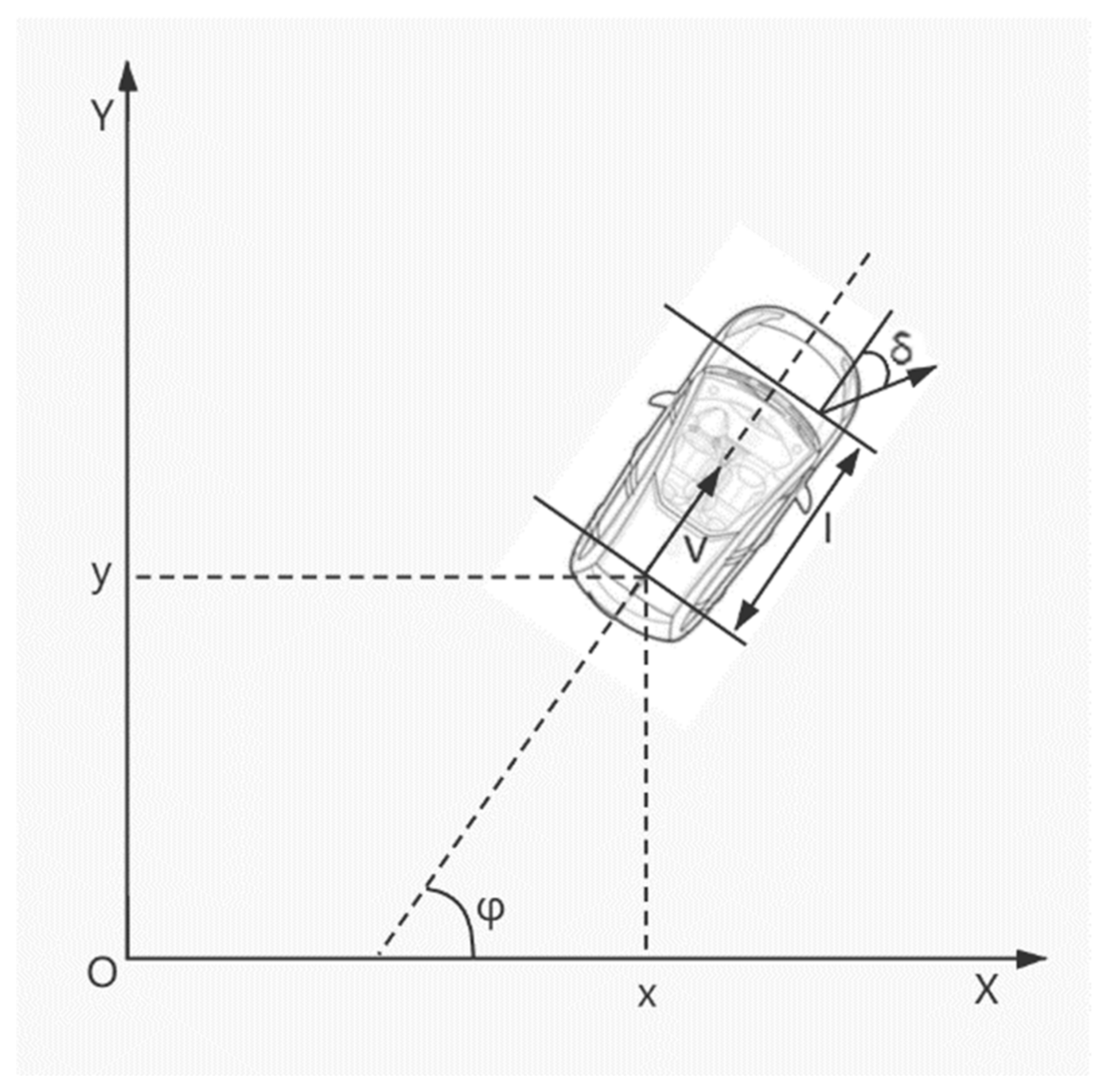
The vehicle kinematics model is shown in Figure 2. The definitions of the main terms appearing in the following equation are shown in

Table 1. Symbols and Definitions.

Symbols	Definitions
$\phi$	Vehicle heading angle
$\delta$	Vehicle front wheel angle
$v$	Vehicle speed
$l$	Wheel base
$u_r$	System reference input
${\chi }_r$	Vehicle reference status
$T$	Sampling time
$Q$	Weight matrix
$R$	Weight matrix
$N_p$	Prediction time domain
$N_c$	Control time domain
$\rho$	Weight coefficient
$\epsilon$	Relaxation factor
$\eta$	Dimension of state quantity
$u_{\min }$	System reference input minimum
$u_{\max }$	System reference input maximum
$\left(X_D,Y_D\right)$	Drift trigger point position
${\psi }_D$	Heading angle of drift trigger point
$d_{thres}$	Drift trigger distance threshold
$\mathsf{\Delta }{\psi }_{thres}$	Drift trigger heading angle threshold
$\mathsf{\Delta }{v}_{thres}$	Drift trigger speed threshold
$l_f$	Distance from centroid to front axle
$l_r$	Distance from centroid to rear axle

.

In the ground fixed coordinate system, the vehicle kinematics equation can be expressed as:

$$\left[\begin{array}{c}\dot{x}\\ \dot{y}\\ \dot{\phi }\end{array}\right]=\left[\begin{array}{c}\cos \phi \\ \sin \phi \\ \raisebox{1ex}{$\tan \delta $}\!\left/ \!\raisebox{-1ex}{$l$}\right.\end{array}\right]v$$

(5)

where $\left(x,y\right)$ is the coordinate of the center of the rear axle of the vehicle, $\phi$ is the vehicle heading angle, $\delta$ is the front wheel angle, $v$ is the longitudinal speed of the vehicle, and $l$ is the wheelbase of the vehicle.

Defining $u(v,\delta )$ as the system input, the state variable is $(x,y,\phi )$. The system can be expressed as:

$$\dot{\chi }=f(\chi ,u)$$

(6)

Each point on the cubic Bessel curve obtained by planning satisfies the above kinematic equation. The reference value is $r$. The reference trajectory can be expressed as:

$${\dot{\chi }}_r=f({\chi }_r,u_r)$$

(7)

The system equation is expanded by the Taylor series at the reference trajectory point:

$${\dot{\chi }}_r=f({\chi }_r,u_r)+\frac{\partial f(\chi ,u)}{\partial x}\left|\chi -{\chi }_r+\frac{\partial f(\chi ,u)}{\partial u}\right|(u-u_r)$$

(8)

where ${\chi }_r=(x_r,y_r,{\phi }_r)$, and $u_r=(v_r,{\delta }_r)$. The error of the vehicle tracking model can be expressed as:

$$\dot{\tilde{\chi }}=\left[\begin{array}{c}\dot{x}-{\dot{x}}_r\\ \dot{y}-{\dot{y}}_r\\ \dot{\phi }-{\dot{\phi }}_r\end{array}\right]=\left[\begin{array}{l}0 0 -v_r\sin {\phi }_r\\ 0 0 v_r\cos {\phi }_r\\ 0 0 0\end{array}\right]\left[\begin{array}{l}\stackrel{}{x}-{\stackrel{}{x}}_r\\ \stackrel{}{y}-{\stackrel{}{y}}_r\\ \stackrel{}{\phi }-{\stackrel{}{\phi }}_r\end{array}\right]+\left[\begin{array}{c}\cos {\phi }_r\\ \sin {\phi }_r\\ \raisebox{1ex}{$\tan {\delta }_r$}\!\left/ \!\raisebox{-1ex}{$l$}\right.\end{array}\begin{array}{c}0\\ 0\\ \raisebox{1ex}{$v_r$}\!\left/ \!\raisebox{-1ex}{$l{\cos }^2{\delta }_r$}\right.\end{array}\right]\left[\begin{array}{l}v-v_r\\ \delta -{\delta }_r\end{array}\right]$$

(9)

We can discretize this equation as:

$$\tilde{\chi }(k+1)=A_{k,t}\tilde{\chi }(k)+B_{k,t}\tilde{u}(k)$$

(10)

where $A_{k,t}=\left[\begin{array}{l}1 0 -v_r\sin {\phi }_{r}T\\ 0 1 v_r\cos {\phi }_{r}T\\ 0 0 1\end{array}\right]$, $B_{k,t}=\left[\begin{array}{l}\cos {\phi }_{r}T 0\\ \sin {\phi }_{r}T 0\\ \raisebox{1ex}{$\tan {\delta }_r$}\!\left/ \!\raisebox{-1ex}{$l$}\right. \raisebox{1ex}{$v_{r}T$}\!\left/ \!\raisebox{-1ex}{$l{\cos }^2{\delta }_r$}\right.\end{array}\right]$, $T$ is the sampling time. In order to ensure that the vehicle can track the cubic Bezier curve quickly and smoothly, the objective function is designed in the following form:

$$J(k)=\sum _{i=1}^{N_p}{\displaystyle \Vert }\eta (k+i|t)-{\eta }_{ref}(k+i|t){{\displaystyle \Vert }}_Q^2+\sum _{i=1}^{N_c-1}{\displaystyle \Vert }\mathsf{\Delta }U(k+i|t){{\displaystyle \Vert }}_R^2+\rho {\epsilon }^2$$

(11)

where $Q$ and $R$ are weight matrices, $N_p$ is the prediction time domain, $N_c$ is the control time domain, $\rho$ is the weight coefficient, and $\epsilon$ is the relaxation factor. The vehicle linear error model is transformed as follows:

$$\xi (k|t)=\left[\begin{array}{l}\tilde{x}(k|t)\\ \tilde{u}(k-1|t)\end{array}\right]$$

(12)

State-space expressions can be expressed as:

$$\xi (k+1|t)={\tilde{A}}_{k,t}\xi (k|t)+{\tilde{B}}_{k,t}\mathsf{\Delta }U(k|t)$$

(13)

$$\eta (k|t)={\tilde{C}}_{k,t}\xi (k|t)$$

(14)

where ${\tilde{A}}_{k,t}=\left[\begin{array}{l}{A}_{k,t} B_{k,t}\\ 0_{m\times n} I_m\end{array}\right]$,${\tilde{B}}_{k,t}=\left[\begin{array}{c}{B}_{k,t}\\ I_m\end{array}\right]$. $n$ is the state quantity dimension and $m$ is the control quantity dimension. The output expression of system prediction can be expressed as:

$$Y(t)={\psi }_t\xi (t|t)+{\mathsf{\Theta }}_t\mathsf{\Delta }U(t)$$

(15)

where $Y_t=\left[\begin{array}{l}\eta (t+1|t)\\ \eta (t+2|t)\\ \eta (t+3|t)\\ \hfill ......\hfill \\ \eta (t+N_p|t)\end{array}\right]$, ${\psi }_t=\left[\begin{array}{c}{\tilde{C}}_{t,t}{\tilde{A}}_{t,t}\\ {\tilde{C}}_{t,t}{\tilde{A}}_{t,t}^2\\ {\tilde{C}}_{t,t}{\tilde{A}}_{t,t}^3\\ .....\\ {\tilde{C}}_{t,t}{\tilde{A}}_{t,t}^{N_p}\end{array}\right]$, $\mathsf{\Delta }{U}_t=\left[\begin{array}{c}\mathsf{\Delta }u(t|t)\\ \mathsf{\Delta }u(t+1|t)\\ \mathsf{\Delta }u(t+2|t)\\ ......\\ \mathsf{\Delta }u(t+N_c|t)\end{array}\right]$, ${\mathsf{\Theta }}_t=\left[\begin{array}{cccc}{\tilde{C}}_{t,t}{\tilde{B}}_{t,t}& 0& 0& 0\\ {\tilde{C}}_{t,t}{\tilde{A}}_{t,t}{\tilde{B}}_{t,t}& {\tilde{C}}_{t,t}{\tilde{B}}_{t,t}& 0& 0\\ ......& ......& ......& ......\\ {\tilde{C}}_{t,t}{\tilde{A}}_{t,t}^{N_c}{\tilde{B}}_{t,t}& {\tilde{C}}_{t,t}{\tilde{A}}_{t,t}^{N_c-1}{\tilde{B}}_{t,t}& ......& {\tilde{C}}_{t,t}{\tilde{A}}_{t,t}{\tilde{B}}_{t,t}\\ ......& ......& ......& ......\\ {\tilde{C}}_{t,t}{\tilde{A}}_{t,t}^{N_p-1}{\tilde{B}}_{t,t}& {\tilde{C}}_{t,t}{\tilde{A}}_{t,t}^{N_p-2}{\tilde{B}}_{t,t}& ......& {\tilde{C}}_{t,t}{\tilde{A}}_{t,t}^{N_p-N_c-1}{\tilde{B}}_{t,t}\end{array}\right]$.

The constraint conditions of both the control quantity and increment are specified. The control quantity includes the wheel angle and the longitudinal speed of the vehicle. The control quantity constraint can be expressed as:

$$u_{\min }(t+k)\le u(t+k)\le u_{\max }(t+k),k=0,1,2\dots N_c-1$$

(16)

The control increment constraint can be expressed as:

$$\mathsf{\Delta }{u}_{\min }(t+k)\le \mathsf{\Delta }u(t+k)\le \mathsf{\Delta }{u}_{\max }(t+k),k=0,1,2\dots N_c-1$$

(17)

The constraint equation for control quantity is transformed and the corresponding transformation matrix is obtained:

$$u(t+k)=u(t+k-1)+\mathsf{\Delta }u(t+k)$$

(18)

$$U_t=1_{N_c}\otimes u(k-1)$$

(19)

$$A=M_{N_c\times N_c}\otimes I_m$$

(20)

where $1_{N_c}$ is a column vector with $N_c$ rows, $M_{N_c\times N_c}$ is the unit lower triangular matrix with dimension $N_c$, $I_m$ is the identity matrix of dimension $m$, $\otimes$ is the Kronecker product, and $u(k-1)$ is the actual control quantity of the previous time. In combination with Equations (18)–(20), the constraint condition of the control quantity can be rewritten as:

$$U_{\min }\le A\times \mathsf{\Delta }{U}_t+U_t\le U_{\max }$$

(21)

where $U_{\min }$ is the minimum set of control variables in the control time domain and $U_{\min }$ is the maximum set of control variables in the control time domain. The objective function is then transformed into a standard quadratic form:

$$J(\xi (t),u(t-1),\mathsf{\Delta }U(t))={\left[\mathsf{\Delta }U{(t)}^T,\epsilon \right]}^T{H}_t\left[\mathsf{\Delta }U{(t)}^T,\epsilon \right]+G_t\left[\mathsf{\Delta }U{(t)}^T,\epsilon \right]$$

(22)

$$\begin{array}{ll}s.t.& \mathsf{\Delta }{U}_{\min }\le \mathsf{\Delta }{U}_t\le \mathsf{\Delta }{U}_{\max }\\ & U_{\min }\le A\mathsf{\Delta }{U}_t+U_t\le U_{\max }\end{array}$$

(23)

where $H_t=\left[\begin{array}{l}{\mathsf{\Theta }}_t^{T}Q{\mathsf{\Theta }}_t+R 0\\ 0 \rho \end{array}\right]$, $G_t=\left[2e_t^{T}Q{\mathsf{\Theta }}_t 0\right]$, $e_t$ is the tracking error in the prediction time domain. In each control cycle, the control input increment can be expressed as:

$$\mathsf{\Delta }{U}_t^{*}={\left[\mathsf{\Delta }{u}_t^{*},\mathsf{\Delta }{u}_{t+1}^{*},\mathsf{\Delta }{u}_{t+2}^{*},\dots ,\mathsf{\Delta }{u}_{t+N_c-1}^{*}\right]}^T$$

(24)

The first element of the optimal sequence control is applied to the control system as the optimal control increment in this cycle, until the next period solves the new optimal control quantity according to the real-time system state. The vehicle finally reaches the drift trigger point, and the vehicle will begin to drift when the drift-triggering condition is met.

3. The Process of Drift Parking

3.1. Drift Open-Loop Control

Vehicle drift is triggered based on the longitudinal coupling characteristics of the tire. According to the tire force ellipse shown in Figure 3, when the rear wheel applies enough braking force to lock the wheel, the longitudinal force reaches the road adhesion limit, and the lateral force provided by the rear wheel is close to zero. At this time, the front wheel turns at a specific angle to produce a lateral force, and the rear wheel cannot provide a balanced lateral force. The lateral force of the front wheel produces a yaw moment on the body, which makes the rear axle sideslip, triggering the drift [19].

To create a sample of drifting instances to study, it is not necessary to float the vehicle into the warehouse during sampling, but only to carry out repeated tail-flick tests of the rear-wheel brake locking in the same field under the same vehicle conditions [20,21]. The vehicle starts in a static state, begins to accelerate, and then applies a drift after reaching a specific speed. Changes in the vehicle state and the action sequence from the initial time of the drift starting to the vehicle coming to a complete stop and achieving stability are recorded, such that:

$$\begin{array}{c}S\left(k\right)=s_1,s_2,\dots s_k\\ A\left(k\right)=a_1,a_2,\dots ,a_k\end{array}$$

(25)

The recorded action $A$ includes the desired steering wheel angle and the desired brake fluid pressure of the vehicle. The recorded vehicle state $S$ includes the $X,Y$ direction coordinates and heading angle. The purpose of state sequence $S\left(k\right)$ is to record the position change at the end of the drift process ($\mathsf{\Delta }X,\mathsf{\Delta }Y$), and the change in the heading angle, $\mathsf{\Delta }\psi$. The absolute coordinates $\left(X_D,Y_D\right)$ and heading angle, ${\psi }_D$, of drift trigger point D can be calculated by using Equation (26) according to the coordinates $\left(X_P,Y_P\right)$ and heading angle (i.e., ${\psi }_P$) of the target location during drift test:

$$\begin{array}{l}{X}_D=X_P+\left(\mathsf{\Delta }X\cos {\psi }_P-\mathsf{\Delta }Y\sin {\psi }_P\right)\\ Y_D=Y_P+\left(\mathsf{\Delta }X\sin {\psi }_P+\mathsf{\Delta }Y\cos {\psi }_P\right)\\ {\psi }_D={\psi }_P-\mathsf{\Delta }\psi \end{array}$$

(26)

The vehicle trajectory and heading sequence are used as the reference sequence in order to monitor whether the vehicle drifts according to the expected trajectory. The drift process failure monitoring strategy outlined in Section 4 was designed based on this premise.

3.2. Design of Drift Trigger Conditions

Directed by the motion tracking controller, the vehicle travels along the planned route and gradually accelerates to the desired speed. When the vehicle is running, the state of the vehicle is monitored in real-time to determine whether it is consistent with the expected drift trigger state. The judgment conditions are as follows:

(1)

Begin by calculating the distance between the current vehicle position coordinates $\left(X,Y\right)$ and the drift trigger point $\left(X_D,Y_D\right)$, $d\left(k\right)=\sqrt{{\left(X-X_D\right)}^2+{\left(Y-Y_D\right)}^2}$. Compare this with the distance obtained previously, to determine if $d\left(k\right)-d\left(k-1\right)\le 0$, and $d\left(k\right)<d_{thres}$. The result indicates whether the vehicle meets the position condition triggered by drift.

(2)

Calculate whether the difference between the actual speed and the expected speed, $\mathsf{\Delta }v$ is less than $\mathsf{\Delta }{v}_{thres}$. If $\mathsf{\Delta }v<\mathsf{\Delta }{v}_{thres}$, the vehicle meets the speed condition triggered by a drift.

(3)

Calculate whether the difference between the actual heading angle and the expected heading angle, $\mathsf{\Delta }\psi$ is less than $\mathsf{\Delta }{\psi }_{thres}$. If $\mathsf{\Delta }\psi <\mathsf{\Delta }{\psi }_{thres}$, the vehicle meets the heading angle condition triggered by drift.

(4)

Judge whether the current steering wheel angle exceeds the limit value. If $\left|\delta \right|<{\delta }_{thres}$, it means that the vehicle meets the yaw motion condition triggered by drift.

Since the vehicle drifting into the warehouse is simulated by the recurrence of the tail-flick action, the motion state cannot be feedback-controlled during drifting with our methodology, so the consistency between the vehicle state at the drift trigger time and the expected vehicle state must be high. If the motion planner or motion tracking controller fails during the depot approach and the vehicle triggers a drift in the wrong state, it will not drift to the depot. It may collide with the pile barrels or other obstacles near the depot, and aggravate the wear of the rear tires. Therefore, it was necessary to design a failure monitoring strategy for the drift entry action. When the vehicle motion state meets the specific conditions and cannot drift into the warehouse successfully, some measures should be taken to stop the drift entry action.

4. Monitoring Strategy

4.1. Supervision Strategy of the Path Planning Algorithm

In this paper, a cubic Bezier curve is used to connect the vehicle starting point and the drift trigger point and serves as the vehicle’s approach path. In the process of generating the path, the algorithm is used to ensure the path has a minimum change in the curvature. In addition to the geometric constraints outlined in the planning stage, the path should also meet the following constraints:

(1)

Maximum curvature constraint: The minimum radius of the path should be greater than the minimum turning radius of the vehicle while satisfying the corner constraint of the path-following controller.

(2)

Maximum attachment constraint: The tire force should be less than the maximum tire force provided by the road surface at the maximum curvature of the constrained path, and also less than the tire force provided at the larger curvature when running at the maximum speed, so as to avoid wheel slip.

(3)

Longitudinal velocity constraint: The planned path should be long enough to allow the vehicle to accelerate at the maximum acceleration and reach the desired drift longitudinal speed at the drift trigger point.

The curvilinear path is treated as being connected by several small circles, and the problem of a vehicle driving along the curvilinear path is simplified as a steady-state circular problem. The relationship between the curvature of the path and the steering angle of the vehicle can now be obtained. If the vehicle maintains a constant speed while moving in a circular motion with a certain radius, $R_0$, then the radius and the front wheel angle of $\delta$ will demonstrate the following relationship:

$$\delta =\left(1+K\cdot v_x^2\right)\frac{l}{R_0}$$

(27)

where $v_x$ is the vehicle speed; $R_0$ is the turning radius; l is the vehicle wheelbase; and $K$ is the stability factor, $K=\frac{m}{l^2}\left(l_f{C}_{\alpha f}-l_r{C}_{\alpha r}\right)$. According to Equation (27), when the front wheel angle ${\delta }_{\max }$ corresponds to the maximum steering wheel angle in the controller constraint, the upper bound of the path curvature constraint is reached when the vehicle reaches maximum speed. In other words, the expression of the maximum curvature constraint is as follows:

$$\kappa \le \frac{k_{\delta }{\delta }_{\max }}{\left(1+K\cdot v_{\max }^2\right)l}$$

(28)

where $k_{\delta }$ is the safety factor, and the value range is [0, 1]. The maximum expected speed on the path is $v_{\max }$, which is equal to the drift trigger speed $v_{\mathrm{target}}$. The vehicle motion is simplified to the steady-state circular driving problem, and the maximum attachment constraint of the path is deduced. The front axle does not slip during steering, provided the following criterion is met:

$$F_{yf}\le \mu F_{zf}$$

(29)

where $\mu$ is the road adhesion coefficient, $F_{yf}$ is front axle lateral force, $F_{zf}$ is front axle vertical force, and $v_y$ is the lateral speed. The vehicle is simplified as a linear model with two degrees of freedom, and the front axle lateral force can be expressed as:

$$F_{yf}=C_{\alpha f}\left(\delta -\frac{v_y+l_f\omega }{v_x}\right)$$

(30)

Due to the steady circular motion of the vehicle:

$$R_0=\frac{v_x}{\omega }$$

(31)

We then substitute Equations (27), (30), and (31) into Equation (29):

$$\kappa \le \frac{\frac{v_y}{v_x}+\frac{\mu F_{zf}}{C_{\alpha f}}}{l\cdot \left(1+K{v}_x^2\right)-l_f}$$

(32)

Ignoring the lateral acceleration of the vehicle makes the inequality constraint stricter, and the maximum path attachment constraint is obtained:

$$\kappa \le \frac{\mu F_{zf}}{C_{\alpha f}\left[l\cdot \left(1+K{v}_x^2\right)-l_f\right]}$$

(33)

When determining the longitudinal speed of the vehicle at a certain point on the path, it is assumed that the vehicle meets the road adhesion and road surface constraints, and thus accelerates with the maximum longitudinal acceleration. The longitudinal speed can then be determined by the distance from the point to the starting point:

$$v_x\left(s\right)=\min \left(v_{\mathrm{target}},\sqrt{2a_{\max }s}\right)$$

(34)

$$a_{\max }=\min \left(\mu g,\frac{T_{\max }i}{mr}\right)$$

(35)

where $v_{\mathrm{target}}$ is the target speed at the drift trigger point, $s$ is the path length from the starting point to a certain point, $T_{\max }$ is the peak torque of the driving motor, $i$ is the transmission ratio of the reduction mechanism, $m$ is the mass of the whole vehicle, and $r$ is the wheel radius.

In addition, it is necessary to verify the distance from the starting point to the drift trigger point in order to ensure that the vehicle can achieve maximum acceleration towards the drift trigger speed before reaching the drift trigger point. The longitudinal speed constraint equation is expressed as follows:

$$s\ge \frac{v_{\mathrm{target}}^2}{2a_{\max }}$$

(36)

where $a_{\max }$ is determined by Equation (35). After planning a path connecting the starting point and the drift trigger point, Equations (28), (33) and (36) can be utilized to check whether the constraint conditions are met, so as to judge the feasibility of the proposed path. If the conditions are not met, it means that the path planning fails. The approach path to the depot must be re-planned by adjusting the initial vehicle position and the initial heading angle.

4.2. Drift Process Monitoring Strategy

The vehicle drift process may be influenced by changes in the vehicle road system, which cause the vehicle system to produce different responses under the same control input. When the same site and the same vehicle conditions are tested, the vehicle road system may change due to factors including:

(1)

Tire characteristics: Tire wear occurs in the process of lock slip, which leads to the change of tire characteristics. The change of tire force will directly affect the corresponding relationship between the steering wheel angle input and the drift trajectory output, so that the actual drift trajectory does not match the expected trajectory.

(2)

Road conditions: Due to the influence of temperature and humidity, the adhesion condition of the road surface may differ between the tail-flick test and the drift test, which changes the tire force under the same load and slip rate.

(3)

Vehicle status: Changes in the vehicle load size and distribution lead to changes in vehicle mass and the centroid position, which affects the tire force.

Through the sampling of vehicle states in the tail-flick test, the expected trajectory and the expected heading angle sequence of the vehicle drift process were obtained. The vehicle state is $\left(X_t,Y_t,{\psi }_t\right)$ at a certain time during the drift. The expected state closest to the current state in the expected sequence is calculated by Equation (37):

$$k=\underset{k}{\arg \min }\left({\left[\begin{array}{c}‖X_t-X_{ref}\left(k\right)‖\\ ‖Y_t-Y_{ref}\left(k\right)‖\\ ‖{\psi }_t-{\psi }_{ref}\left(k\right)‖\end{array}\right]}^{\mathrm{T}}\times \left[\begin{array}{ccc}{\omega }_X& & \\ & {\omega }_Y& \\ & & {\omega }_{\psi }\end{array}\right]\times \left[\begin{array}{c}‖X_t-X_{ref}\left(k\right)‖\\ ‖Y_t-Y_{ref}\left(k\right)‖\\ ‖{\psi }_t-{\psi }_{ref}\left(k\right)‖\end{array}\right]\right)$$

(37)

where ${\omega }_X$,${\omega }_Y$, and ${\omega }_{\psi }$ are the weight coefficient, which is used to balance the influence of different distance and angle dimensions. After obtaining the expected state at the current moment, the weighted error vector between the actual vehicle state and the expected state at the current moment is calculated:

$${\mathit{e}}_t={\left[{\omega }_X,{\omega }_Y,{\omega }_{\psi }\right]}^{\mathrm{T}}·\left[\begin{array}{c}‖X_t-X_{ref}\left(k\right)‖\\ ‖Y_t-Y_{ref}\left(k\right)‖\\ ‖{\psi }_t-{\psi }_{ref}\left(k\right)‖\end{array}\right]$$

(38)

The error vector ${\mathit{e}}_t$ is compared with the error threshold vector ${\mathit{e}}_{thres}={\left[e_{thres}^X,e_{thres}^Y,e_{thres}^{\psi }\right]}^{\mathrm{T}}$. When any component of ${\mathit{e}}_t$ is greater than y, it is considered that the control open-loop is invalid and the vehicle cannot accurately stop in the storage position.

5. Simulation and Ground Test

A CarSim-Simulink simulation platform was built to verify the effectiveness of the drift parking algorithm, and the drift parking action in the simulation environment was realized. Key parameters of the vehicle model are shown in

Table 2. CarSim key parameters of simulation vehicle model.

Parameter	Unit	Value	Parameter	Unit	Value
Vehicle mass	kg	1412	Vehicle length	m	4.025
Yaw moment of inertia	kg m2	1536.7	Vehicle width	m	1.916
Wheel radius	m	0.325	Steering ratio	-	2.91
Centroid height	m	0.54	Wheelbase	m	2.91

.

5.1. Simulation Test of Drift Whole Process Control

A simulation experiment of the whole-process open-loop algorithm was carried out to verify the effectiveness of the algorithm.

(1)

Working condition setting:

The location coordinates of the vehicle’s starting point are (−100, −50), and the location coordinates of the depot are (0, 0). The initial vehicle heading angle is 0°. The initial speed is 0 km/h. The target location’s orientation is 180°. The road adhesion coefficient is 1. According to the results of the tail-flick test, the preset coordinates of the drift trigger point are (−10.69, −6.13), and the heading angle of the drift point is 7.50°. The longitudinal speed triggered by the drift is 39.96 km/h, and the step angle of the drift steering wheel is 140°.

(2)

Parameter setting:

The threshold settings of the drift trigger point are $\mathsf{\Delta }{v}_{thres}=0.5 \text{km/h}$, $d_{thres}=0.3 \mathrm{m}$, ${\psi }_{thres}=5$, and ${\delta }_{thres}=5$.

(3)

Simulation test results:

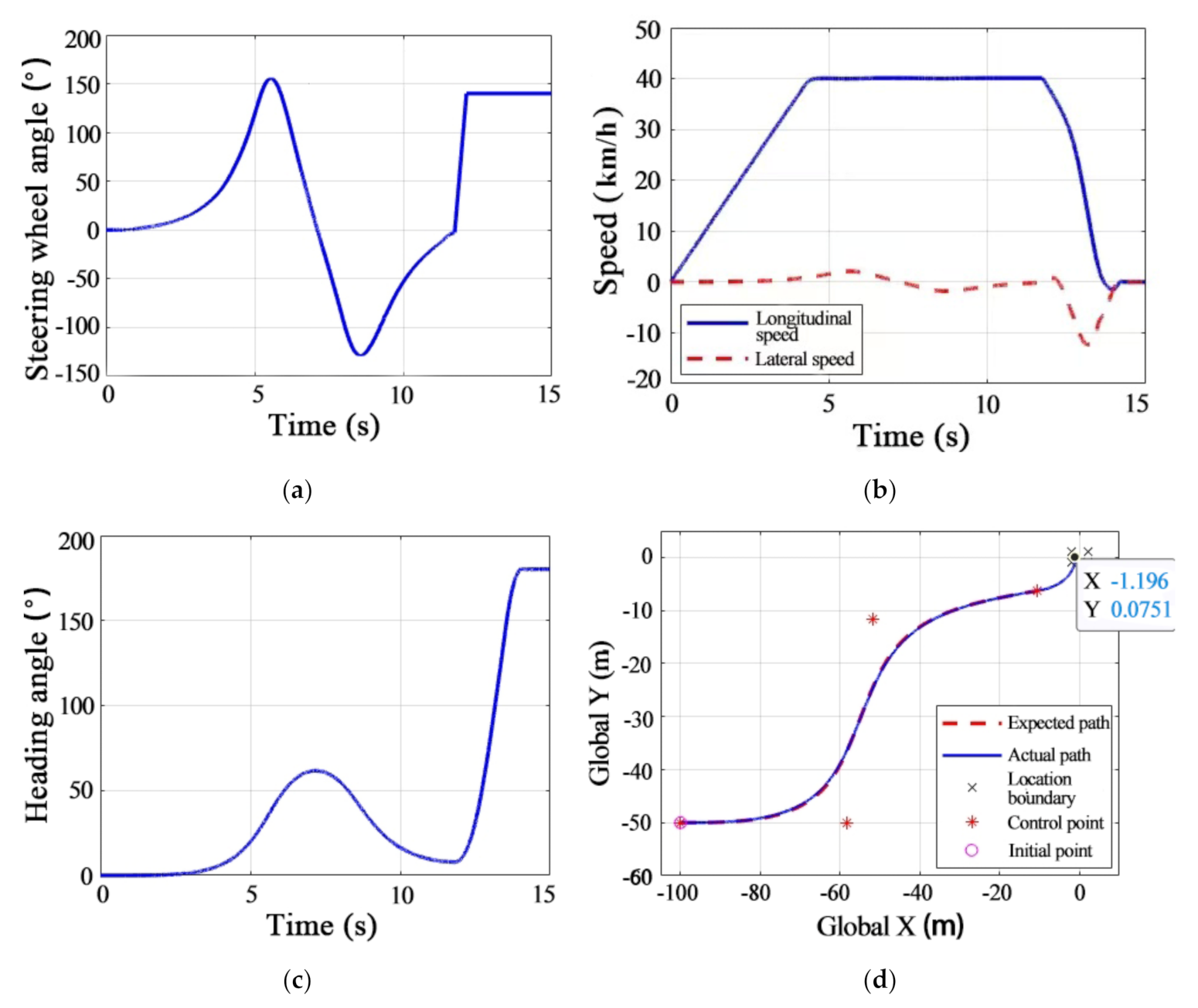
The simulation results are shown in Figure 4. At 11.72 s, when the vehicle reaches (−10.97, −6.34), the vehicle is 0.278 m away from the drift trigger point, and the steering wheel angle is −2.7°. The longitudinal speed is 40.1 km/h, satisfying the drift triggering condition. The change in the vehicle trajectory in the global coordinate system is shown in Figure 4. Finally, the vehicle parks at (−1.196, 0.075). The distance from the center of the warehouse’s error is 0.196 m. The final heading angle is 180.2°, and the error of the storage location orientation angle is 0.2°. The location is 5.2 × 2.5 m in size. The simulation test demonstrates that the car body stops completely within the storage position range and does not interfere with the storage position line. An animation of the entire output process made in CarSim is shown in Figure 5. The figures demonstrate that the vehicles are correctly parked in the warehouse and surrounded by the four pile barrels.

5.2. Function Verification of Monitoring Strategy

First, the initial positions and heading angles of different vehicles are set to verify the effectiveness of the failure monitoring strategy of the path planner. The simulation results are shown in Figure 6. The coordinates of the target drift trigger point are (0, 0), and the heading angle of the drift trigger point is 0°. The three flag bits correspond to the maximum curvature constraint, the maximum adhesion constraint, and the longitudinal speed constraint, respectively. The path planning and feasibility judgment were completed before the simulation test.

As shown in Figure 6a,b, the vehicle initial point coordinates are (−100, −50), and the initial heading angle is 0°. The simulation results show that the vehicle can complete the approach action, and the failure flag is 0.

As shown in Figure 6c,d, the vehicle initial point coordinates are (−10, −10), and the initial heading angle is 90°. the path is too short for the vehicle to accelerate to the desired drift trigger speed by the time it reaches the desired point, and thus does not meet the drift trigger conditions. The path does not meet the longitudinal speed constraint, and the corresponding flag bit is 1.

As shown in Figure 6e,f, the vehicle initial point coordinates are (−100, −50), and the initial heading angle is 180°. Due to the path’s large curvature, the vehicle cannot track the path with the maximum steering wheel angle, which leads to path tracking failure. The path does not satisfy the maximum curvature constraint, and the corresponding flag bit is 1.

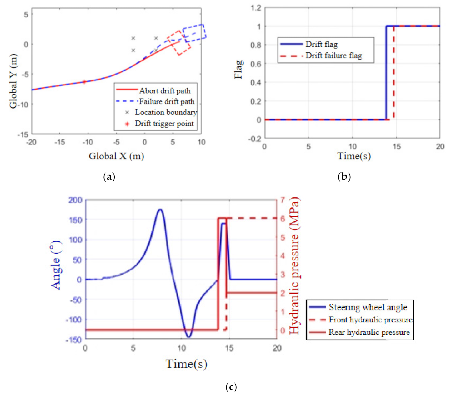
Next, the drift trajectory tracking and monitoring strategy and drift stop strategy are simulated and verified. Let the weight coefficients in Equation (38) be ${\omega }_X=1$, ${\omega }_Y=1$, ${\omega }_{\psi }=2$. The target location is (0, 0), and the heading angle of the target location is 180°. The vehicle starting point coordinates are (−100, −50), and the starting heading angle is 0°. If the road adhesion coefficient is set to 0.5, the vehicle can complete the approaching movement on the road surface attached to the center, but it cannot drift into the warehouse according to the open-loop control law obtained from the tail-flick test when the adhesion coefficient is 1. The simulation results are shown in Figure 7. As can be seen from Figure 7b, at 13.84 s, the vehicle meets the drift trigger condition and enters the drift state. At 14.71 s, the controller detects that the vehicle deviates from the expected drift trajectory, and the drift failure flag is 1. At this time, the steering wheel angle returns to 0°. The front axle is put under greater pressure and the pressure on the rear axle is reduced, as shown in Figure 7c. Figure 7a shows that the drift stop action makes the vehicle stop faster and greatly reduces the yaw motion. Compared with a vehicle completing the entire drift the final heading angle changed from 193° to 124°, the total drift time decreased from 5.86 s to 3.56 s, and the rear wheel slip distance decreased from 28.87 m to 23.33 m. The simulation results verify the effectiveness of the strategy.

5.3. Ground Test

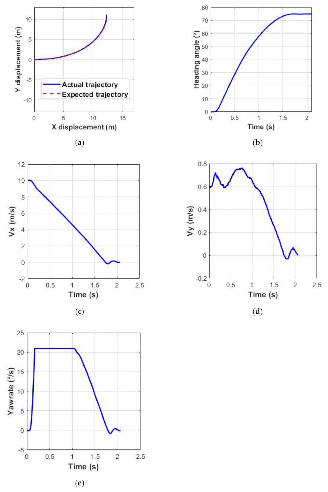
The open-loop control drift algorithm was verified using the actual vehicle. First, a 170° steering wheel angle was applied to record the change in the vehicle motion state from the beginning to the end of the drift. The initial position of the vehicle is (0, 0). At the end of the drift, the x-direction displacement changes by 12.27 m, the y-direction displacement changes by 11.28 m, and the heading angle changes by 75.4 degrees. In the real vehicle test, the vehicle conditions and road conditions must be consistent to achieve high-precision drift control. The data begin recording when the drift state is triggered. The change in vehicle motion state parameters across the entire drift process is shown in Figure 8.

The drift trigger point is set to (0, 0), the distance threshold of the drift trigger point is set to 0.3 m, and the heading angle error threshold is set to 3 degrees. The vehicle meets the drift trigger condition and begins to drift. During the entire process of the vehicle drifting and entering the warehouse, the heading angle changes by 75.1°, the x-direction displacement changes by 12.32 m, and the y-direction displacement changes by 11.05 m. In contrast to the collected data, the heading angle deviation is 0.3°, the x-direction displacement deviation is 0.05 m, the y-direction displacement deviation is 0.23 m, and the vehicle completes the drift.

6. Discussion and Conclusions

The actual vehicle test is compared with the simulation experiment. In the simulation experiment, the distance between the drifting vehicle and the center of the parking location is 0.196 m. In the actual vehicle test, when the vehicle completes its drift, the distance between the vehicle and the center of the parking location is 0.235 m. This indicates a 3.9% accuracy difference between the two. The accuracy of the heading angle deviation is 1%. These differences stem from fluctuations in the drift trigger point and the state of the vehicle road system during the actual vehicle test.

In this paper, a segmented drift algorithm is designed to extend the handling ability beyond the limit of vehicle stability. By tracking the planned path, the vehicle can reach the drift trigger point and apply the open-loop control rate. In the simulation test, the vehicle drifts into the parking location from 0.196 m away, with a heading angle deviation of 0.2 degrees. In the ground test, the deviation between the final position of the vehicle and the center position of the parking location is 0.235 m, and the deviation of the heading angle is 0.3°. A strategy for monitoring the drift triggering condition, path planning, and vehicle state was designed. The simulation results show that the monitoring method can accurately monitor the real-time state of the vehicle and completion of the drift. The simulation and real vehicle test results show that the segmented drift control method can achieve high-precision drift parking.

The research of segmented drift control has the following significance:

(1)

Through the combination of path planning, path tracking, and an open-loop control algorithm, it can realize the action of the driverless vehicle drifting into the warehouse, which demonstrates the potential of further research on driverless vehicle under extreme conditions.

(2)

The segmented drift control strategy is designed to make the vehicle complete a drift during its approach of the warehouse. In order to ensure that there are no major changes to the vehicle road system, the open-loop control rate can effectively complete the drift.

(3)

The realization of the whole drift process requires the initial state of the vehicle and the vehicle path system to be consistent with the acquisition path, which leads to the low success rate of drift parking. Constraints on the planned path and drift trigger state can significantly improve the success rate of drift storage. The monitoring strategy of the drift process can also ensure the integrity and safety of the test.

In subsequent research based on this paper, the tire inflation state should also be fully considered as part of the road system. The tire characteristics and road adhesion coefficient could be used as input for improving the robustness of the system. Future research could try to employ reinforcement learning methods in drift control experiments.

References

- Zhang, F. Trajectory Planning and Motion Control for Extreme Maneuvers of Autonomous Vehicles. Ph.D. Thesis, Tsinghua University, Beijing, China, 2018. [Google Scholar]
- Goh, J.Y.; Goel, T.; Gerdes, J.C. A controller for automated drifting along complex trajectories. In Proceedings of the 14th International Symposium on Advanced Vehicle Control (AVEC 2018), Beijing, China, 14–18 September 2018; pp. 1–6. [Google Scholar]
- Alcala, E.; Puig, V.; Quevedo, J.; Escobet, T.; Comasolivas, R. Autonomous vehicle control using a kinematic Lyapunov-based technique with LQR-LMI tuning. Control Eng. Pract. 2018, 73, 1–12. [Google Scholar] [CrossRef]
- Tagne, G.; Talj, R.; Charara, A. Higher-order sliding mode control for lateral dynamics of autonomous vehicles, with experimental validation. In Proceedings of the IEEE Intelligent Vehicles Symposium, Gold Coast, QLD, Australia, 23–26 June 2013; pp. 678–683. [Google Scholar]
- Hu, C.; Wang, R.; Yan, F. Integral Sliding Mode-Based Composite Nonlinear Feedback Control for Path Following of Four-Wheel Independently Actuated Autonomous Vehicles. IEEE Trans. Transp. Electrif. 2016, 2, 221–230. [Google Scholar] [CrossRef]
- Funke, J.; Brown, M.; Erlien, S.M.; Gerdes, J.C. Collision Avoidance and Stabilization for Autonomous Vehicles in Emergency Scenarios. IEEE Trans. Control Syst. Technol. 2017, 25, 1204–1216. [Google Scholar] [CrossRef]
- Liu, K.; Gong, J.; Kurt, A.; Chen, H.; Ozguner, U. Dynamic Modeling and Control of High-Speed Automated Vehicles for Lane Change Maneuver. IEEE Trans. Intell. Veh. 2018, 3, 329–339. [Google Scholar] [CrossRef]
- Guo, J.; Luo, Y.; Li, K.; Dai, Y. Coordinated path-following and direct yaw-moment control of autonomous electric vehicles with sideslip angle estimation. Mech. Syst. Signal Process. 2018, 105, 183–199. [Google Scholar] [CrossRef]
- Kim, E.; Kim, J.; Sunwoo, M. Model predictive control strategy for smooth path tracking of autonomous vehicles with steering actuator dynamics. Int. J. Automot. Technol. 2014, 15, 1155–1164. [Google Scholar] [CrossRef]
- Velenis, E.; Katzourakis, D.; Frazzoli, E.; Tsiotras, P.; Happee, R. Steady-state drifting stabilization of RWD vehicles. Control Eng. Pract. 2011, 19, 1363–1376. [Google Scholar] [CrossRef]
- Nakano, H.; Kinugawa, J.; Kosuge, K. Control of a four-wheel independently driven electric vehicle with a large sideslip angle. In Proceedings of the 2014 IEEE International Conference on Robotics and Biomimetics (ROBIO 2014), Bali, Indonesia, 5–10 December 2014; pp. 265–270. [Google Scholar]
- Goh, J.Y.; Gerdes, J.C. Simultaneous stabilization and tracking of basic automobile drifting trajectories. In Proceedings of the IEEE Intelligent Vehicles Symposium, Gothenburg, Sweden, 19–22 June 2016; pp. 597–602. [Google Scholar]
- Jelavic, E.; Gonzales, J.; Borrelli, F. Autonomous Drift Parking using a Switched Control Strategy with Onboard Sensors. IFAC-PapersOnLine 2017, 50, 3714–3719. [Google Scholar] [CrossRef]
- Kolter, J.Z.; Plagemann, C.; Jackson, D.T.; Ng, A.; Thrun, S. A probabilistic approach to mixed open-loop and closed-loop control, with application to extreme autonomous driving. In Proceedings of the IEEE International Conference on Robotics Automation, Anchorage, AK, USA, 3–7 May 2010; pp. 839–845. [Google Scholar]
- Kolter, J.Z. Learning and Control with Inaccurate Models; Stanford University: San Francisco, CA, USA, 2010. [Google Scholar]
- Sakurama, K.; Nakano, K. Path tracking control of Lagrange systems with obstacle avoidance. Int. J. Control Autom. Syst. 2012, 10, 50–60. [Google Scholar] [CrossRef]
- Rosolia, U.; De Bruyne, S.; Alleyne, A.G. Autonomous vehicle control: A nonconvex approach for obstacle avoidance. IEEE Trans. Control Syst. Technol. 2016, 25, 469–484. [Google Scholar] [CrossRef]
- Gong, J.; Liu, K.; Qi, J. Model Predictive Control for Self-Driving Vehicles, 2nd ed.; Beijing Institute of Technology Press: Beijing, China, 2019; pp. 89–90. [Google Scholar]
- Zhang, F.; Gonzales, J.; Li, S.; Borrelli, F.; Li, K. Drift control for cornering maneuver of autonomous vehicles. Mechatronics 2018, 54, 167–174. [Google Scholar] [CrossRef]
- Gonzales, J.M. Planning and Control of Drift Maneuvers with the Berkeley Autonomous Race Car. Ph.D. Thesis, University of California, Berkeley/San Francisco, CA, USA, 2018. [Google Scholar]
- Lau, T.K. Learning autonomous drift parking from one demonstration. In Proceedings of the 2011 IEEE International Conference on Robotics Biomimetics, Karon Beach, Thailand, 7–11 December 2011; pp. 1456–1461. [Google Scholar]
Figure 1.
Schematic diagram of drift parking.
Figure 2.
Kinematic model.
Figure 3.
Tire force friction ellipse.
Figure 4.
Simulation test results: (a) Steering wheel angle; (b) Vehicle speed; (c) Heading angle; and (d) Drift process.
Figure 5.
Drift parking process.
Figure 6.
Simulation test of path planning failure monitoring strategy: (a) Vehicle path; (b) Failure flag; (c) Vehicle path; (d) Failure flag; (e) Vehicle path; and (f) Failure flag.
Figure 7.
Simulation test of drift process failure monitoring strategy: (a) Vehicle path; (b) Drift flag; and (c) Actuator output.
Figure 8.
Ground test: (a) Vehicle path; (b) Heading angle; (c) Vx; (d) Vy; and (e) Yawrate.