Article

Lake Ecosystem Robustness and Resilience Inferred from a Climate-Stressed Protistan Plankton Network

1
Department of Ecology, University of Kaiserslautern, D-67633 Kaiserslautern, Germany
2
Limnological Station, Department of Plant and Microbial Biology, University of Zurich, CH-8802 Zurich, Switzerland
3
Laboratory of Soil Biodiversity, University of Neuchâtel, CH-2000 Neuchâtel, Switzerland
4
Research Department for Limnology, University of Innsbruck, A-5310 Mondsee, Austria
*
Author to whom correspondence should be addressed.
Submission received: 30 January 2021 / Revised: 17 February 2021 / Accepted: 1 March 2021 / Published: 6 March 2021

Abstract

:
Network analyses of biological communities allow for identifying potential consequences of climate change on the resilience of ecosystems and their robustness to resist stressors. Using DNA metabarcoding datasets from a three-year-sampling (73 samples), we constructed the protistan plankton co-occurrence network of Lake Zurich, a model lake ecosystem subjected to climate change. Despite several documentations of dramatic lake warming in Lake Zurich, our study provides an unprecedented perspective by linking changes in biotic association patterns to climate stress. Water temperature belonged to the strongest environmental parameters splitting the data into two distinct seasonal networks (October–April; May–September). The expected ecological niche of phytoplankton, weakened through nutrient depletion because of permanent thermal stratification and through parasitic fungi, was occupied by the cyanobacterium Planktothrix rubescens and mixotrophic nanoflagellates. Instead of phytoplankton, bacteria and nanoflagellates were the main prey organisms associated with key predators (ciliates), which contrasts traditional views of biological associations in lake plankton. In a species extinction scenario, the warm season network emerged as more vulnerable than the cold season network, indicating a time-lagged effect of warmer winter temperatures on the communities. We conclude that climate stressors compromise lake ecosystem robustness and resilience through species replacement, richness differences, and succession as indicated by key network properties.

1. Introduction

Protists are essential for lake ecosystems because their roles as primary producers, decomposers, or consumers contribute to biomass fluxes among different trophic levels [1,2]. Such interactions are essential components that define the function of an ecosystem. A major challenge in revealing the complexity of these interactions is to account for the temporal shift in protistan community structures. Species replacement, changes in species richness differences, and succession in protistan communities are largely triggered by natural changes of environmental conditions (such as seasonal changes) and stressors (such as pollution or climate change stressors) [3,4,5,6,7,8]. Singular samplings of individual sites only provide a snapshot of a specific moment in time of the protistan community under study, and, therefore, do not allow to infer the complex interactions in these communities and their reaction to habitat changes. Addressing such topics requires data collected in time-series studies [9]. To date, the vast majority of time-series studies of protistan freshwater communities were dedicated to the analysis of alpha- and beta-diversity patterns [10,11] but provided only a limited perspective on the consequences of environmental changes and stressors on biotic associations within communities. Such associations and their persistence under environmental changes, however, are a powerful indicator to assess the resilience and robustness of an ecosystem affected by these changes [12]. Thereby, ecosystem robustness describes the resistance of a community to maintain its functioning during a disturbance by stressors (that is, its buffering capacity during e.g., periods of warming), while resilience describes the reorganization of a community back to a stable state after disturbance by stressors [13,14,15].
A statistical approach to infer potential biological associations from time-series data are co-occurrence network analyses [12,16,17,18,19,20,21,22]. The basic prerequisite of co-occurrence analyses is the following: two organisms which are ecologically associated are highly likely to express their relation in significantly correlating abundance profiles [16]. Co-occurrence networks are not capable to characterize the underlying reasons for specific associations between individual species but efficient in inferring effects of natural and stressor-induced changes on ecosystem function and robustness [12,23,24,25,26,27]. Towards this goal, several measures from graph theory can be considered. Centrality measurements or articulation points of networks identify keystone species, i.e., species whose loss would cause severe effects because they fulfill important functions in a community [28,29,30]. Of special importance in this context are species involved in three-way-associations, because such patterns are promising indicators for the structure and function of microbial ecosystems [16]. Modularity evaluates how far a network is divided into densely interconnected groups [31,32,33]. High modularity indicates that a community comprises multiple functional guilds or multiple ecological niches within which organisms are more frequently associated than between the different functional guilds or ecological niches [33,34]. Average path length, average degree, and density inform about the tightness of association patterns [35,36,37]. The higher these measures the more associations between community members are established and, consequently, the more (functional) redundancy exists. Robustness, measured via a loss of connectivity, indicates a network’s response towards disturbances that would remove key species from a community [38,39,40,41].
In marine [26,42,43] and soil environments [23,24,44], network analyses were successfully exploited to analyze the resilience of microbial communities when subjected to climate change stressors. Similar studies on protistan plankton are rare for freshwater ecosystems in general, and lakes in specific. Our study aims at filling this void by analyzing the protistan plankton co-occurrence network of a large freshwater lake, subjected to climate change effects. Located in the northern part of the European Alps, Lake Zurich is a model ecosystem for temperate European lakes [45]. Numerous studies documented the impacts of global warming and anthropogenic stressors on Lake Zurich and the resulting dramatic ecosystem changes including economic consequences [45,46,47,48,49]. A major effect on protistan plankton communities triggered by lake warming in Lake Zurich is a decline in phytoplankton diversity and biomass as a result of a changing mixing behavior of the lake’s water layers that led to an interruption of nutrient cycling [45,46].
We inferred the protistan plankton co-occurrence network of the epilimnion in Lake Zurich (hereafter referred to as the protistan plankton community network) from a three-year time-series DNA metabarcoding dataset with biweekly sampling. Analyzing network key properties, we addressed the following questions: (i) How are environmental parameters, which are linked to climate change in Lake Zurich, involved in association patterns within the protistan plankton communities? (ii) Do changes in phytoplankton diversity lead to changes in association patterns within protistan plankton communities of Lake Zurich that deviate from predictions of traditional models (such as the Plankton Ecology Group Model, PEG [3,4])? (iii) How does lake warming affect the robustness and resilience of protistan planktonic community associations, and, thus, ecosystem response in Lake Zurich?

2. Materials and Methods

2.1. Sampling Site Information and Measurement of Environmental Parameters

Plankton samples of Lake Zurich, Switzerland (47°19.3′ N, 8°33.9′ E) were collected biweekly from the pelagic zone of the epilimnion in a depth of 5 m between March 2014 and February 2017, resulting in a dataset of 73 samples. All samples were processed as previously described in Qu et al. [50]. Raw water samples had a volume of 5 L and were split into 2 L sample duplicates, while the remaining sample was used for determining biotic and abiotic environmental parameters. Each 2 L sample duplicate was pre-filtered through a 150 µm net to remove larger zooplankton, then filtered onto a 0.65 µm membrane filter (Durapore; Merck Millipore, Darmstadt, Germany) using a peristaltic pump. Filters containing planktonic organisms in the targeted size range of 0.65–150 µm were immediately transferred into a cryovial containing 1.5 mL RNALater (Qiagen, Hilden, Germany), placed in a refrigerator overnight, and stored at −80 °C until further processing.
Environmental parameters were measured for each sample (Table 1 and Table S1). Water temperature (°C), oxygen concentration (mg L−1), oxygen saturation (%), and conductivity (µS cm−1) were measured in situ with a multiparameter probe (6600 V2; Yellow Springs Instruments, Yellow Springs, OH, USA). Irradiance (i.e., photosynthetic active radiation; µmol m−2 s−1) was measured with a spherical underwater quantum sensor (LI-COR, Bad Homburg, Germany). Secchi depth (m) was determined with a Secchi disk. Total in situ chlorophyll concentrations and in situ chlorophyll concentrations assigned to specific phototrophic groups (diatoms and cryptophytes) were measured with a TS-16-12 fluoroprobe (bbe Moldaenke, Kronshagen, Germany). Additionally, the fluoroprobe was calibrated for the quantification of the phycoerythrin-containing cyanobacterium Planktothrix rubescens. For bacteria and coccoid cyanobacteria counts, 40 mL of each sample were preserved with formaldehyde (2% final concentration), stained with SYBR-Green I (Sigma-Aldrich, St. Louis, MO, USA), and evaluated via flow cytometry (Cytoflex S; Beckman Coulter, Brea, CA, USA) [51]. Through manual gating of scatterplots, the total bacterial abundance could be further differentiated into low nucleic acid bacteria and high nucleic acid bacteria [52].
Physical and chemical parameters give the average, minimum, and maximum determined during the investigation period March 2014 to February 2017 for the sampling depth in 5 m. Chemical parameters (marked with *) were determined every month (n = 36) by Water Supply Zurich, physical parameters were determined on a biweekly basis (n = 72).

2.2. Sample Processing and High-Throughput Sequencing

Each filter was placed into a lysing matrix tube (Lysing Matrix E; MP Biomedicals, Illkirch, France) into which 600 µL RLT buffer (Qiagen) and 6 µL β-Mercaptoethanol were inserted. After a centrifugation step, the supernatant was discarded and the pellet was suspended in 200 µL RLT buffer and 2 µL β-Mercaptoethanol. Subsequently, each matrix tube was subjected to bead-beating for 45 s by 30 Hz (MM 200; Retsch, Haan, Germany). Total DNA was extracted using the AllPrep DNA/RNA Mini Kit (Qiagen). From the extracted DNA we amplified the hypervariable V9 region of the 18S rDNA following a standard protocol [53]. The protocol employed 1391F as a forward primer (5′-GTACACACCGCCCGTC-3′; [54]) and EukB as a reverse primer (5′-TGATCCTTCTGCAGGTTCACCTAC-3′; [55]). The PCR protocol consisted of an initial denaturation step at 98 °C for 30 s, followed by 30 cycles of 10 s at 98 °C, 20 s at 61 °C, 25 s at 72 °C, and a final five-minute extension at 72 °C. The reactions volumes amounted to 50 µL and included 0.5 µL Phusion polymerase (New England Biolabs (NEB), Ipswich, MA, USA), 10 µL 5xPhusion GC buffer (NEB), 1 µL 10 mM dNTPs, 0.5 µL template DNA, 32.5 µL pure water, and 0.5 µL of each forward and reverse primer. Triplicate PCR reactions were run for each DNA extract to minimize PCR bias. Prior to purification (MinElute Kit; Qiagen), PCR sample replicates were pooled.
To prepare the resulting PCR products for high-throughput sequencing (HTS), sequencing libraries were constructed using the NEB Next Ultra DNA Library Prep Kit for Illumina (NEB). Library quality was assessed with an Agilent Bioanalyzer 2100 system (Agilent, Santa Clara, CA, USA). Illumina MiSeq sequencing was conducted by SeqIT GmbH & Co. KG (Kaiserslautern, Germany). The sequence data files are deposited at the Sequence Read Archive of the National Center for Biotechnology Information under project number PRJNA609412.

2.3. Sequence Quality Control, Clustering, and Taxonomic Assignment

A multiple-step pipeline was employed for identifying high-quality sequences. First, excessive primer overhangs were clipped using CUTADAPT version 1.18 [56]. Clipped sequences were then quality-checked in QIIME version 1.8.0 [57] by selecting sequences that had exactly matching barcodes and primers, contained exclusively unambiguous nucleotides, and had a minimum length of 90 nucleotides. Finally, all sequences were de novo chimera-checked using UCHIME version 5.2.236 [58]. Since efficient sequence clustering is extremely beneficial for subsequent network analyses [19], we applied a two-level clustering approach to all high-quality HTS sequences [59]. This strategy diminished the extent of placing highly similar sequences, arising from intra-individual or intra-species genetic variation, into distinct operational taxonomic units (OTUs). Without this precaution, false-positive signals are prone to inflate the number of nodes and edges in the networks, as several OTUs representing the same species are highly likely to significantly co-occur in time-series data. The first level of clustering was conducted in Swarm version 2.2.2 with d = 1 and the fastidious option -f [60]. For second-level clustering, the representative sequences of all swarms were extracted and pairwise aligned in VSEARCH version 2.11.0 [61]. The result of the pairwise sequence analysis was used to create sequence similarity networks of the representative sequences at a threshold of 97% sequence similarity. Network sequence clusters (NSCs) created by this second level of clustering represented the units for all downstream analyses.
NSCs with a total abundance of fewer than three sequences were discarded. The most abundant sequence of each remaining NSC (n = 37,848) was extracted and used for taxonomic assignment in BLAST against NCBIs GenBank release version 226.0. For placement of BLAST hits into higher taxonomic groups, we considered the BLAST hit with the highest sequence similarity and e-value and followed the classification system in Adl et al. [62]. Only NSCs with a representative sequence that shared a fragment of at least 90 consecutive nucleotides and a sequence similarity of at least 80% to any hit in GenBank were retained. If the best hit in GenBank related to an unidentified environmental reference sequence, we checked whether that reference sequence was also part of the protist ribosomal reference (PR2) database version 4.11.0 [63] and adopted the taxonomic affiliation. Although PR2 is a subset of GenBank, it is a curated database that contains taxonomic affiliations for several entries which are merely listed as environmental reference sequences in GenBank.

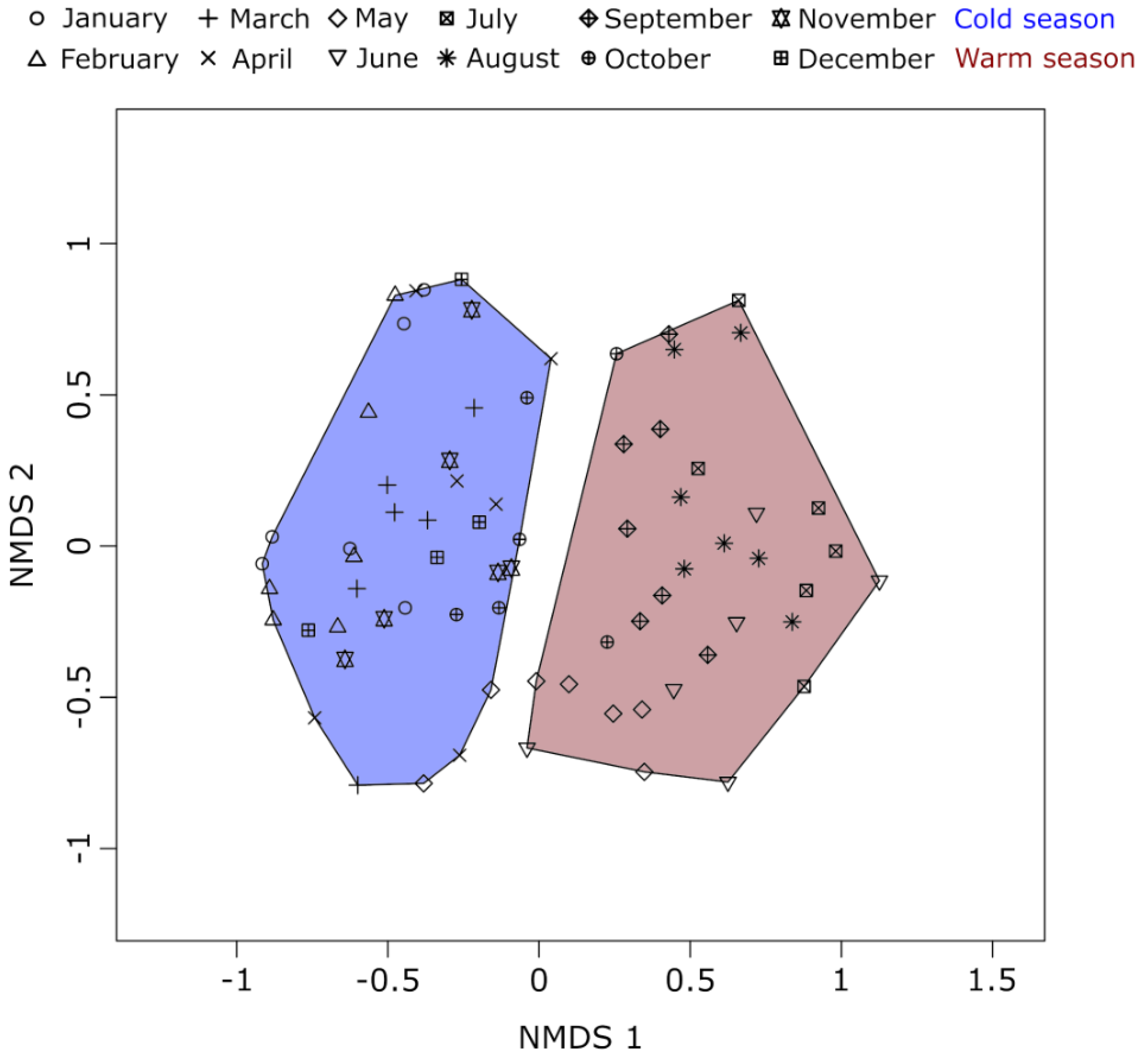
2.4. Compositional Variation Analyses

For revealing general seasonal succession patterns in the sampled data, two independent non-metric multidimensional scaling (NMDS) analyses were performed in R version 3.5.1 [64] using the package “vegan” version 2.5.2 [65]. By default, NMDS calculations in vegan include a two-level normalization step of data in the input matrix: first a Wisconsin double standardization is performed, then a square root transformation. In the first NMDS, samples were analyzed according to their community composition and in the second NMDS (Figure S1), samples were analyzed according to their environmental parameter profile (Table S1). Both NMDS analyses employed Bray–Curtis dissimilarity scores between all pairs of samples. Because seasonality emerged as the major structuring factor, we classified samples for subsequent network analyses into two groups. One “cold season” dataset of 38 samples (October–April; with the exception of samples 04/01/15 and 10/12/16) and one “warm season” dataset of 35 samples (May–September).

2.5. Construction of Co-Occurrence Networks

Protistan plankton co-occurrence networks were calculated in NetworkNullHPC version 0.3 (https://github.com/lentendu/NetworkNullHPC, accessed on 30 January 2021; [66]), a script specifically designed after the null model strategy for inferring statistically significant co-occurrences in metabarcoding datasets [16]. Data preparation in NetworkNullHPC started by removing low-abundant NSCs which occurred in less than 10% of the samples from the OTU-to-sample read abundance matrix. The resulting data matrix was log-ratio normalized, which is highly recommended for compositional data [67]. Following this recommendation, read abundances were log-transformed and then normalized by the read abundances per sample, under consideration of the expected sequencing depth. Null models were generated from the normalized read abundance matrix by adding random low-level noise in 1000 permutations to obtain statistically significant thresholds of Spearman’s rank correlation coefficient (rho). In addition, only nodes and edges which were persistently detected in the majority of permutations were retained for creating a consensus network (see [16] and [66] for detailed descriptions of the complete null model strategy). This approach avoids arbitrary set thresholds for Spearman’s rho and instead determines dataset-specific thresholds. In our study, the statistically determined Spearman’s rho threshold for co-occurrence was set to 0.6 in the cold season network and 0.62 in the warm season network, and −0.59 and −0.61 in co-exclusion networks, respectively. Correlations between NSCs that exceeded the co-occurrence or co-exclusion threshold were included in the resulting consensus network (one for the cold season, one for the warm season) in which they formed the nodes (NSCs) and edges (significant correlations). We further enabled NetworkNullHPC’s -e option to include environmental parameters in the network correlation analyses. The networks were visualized in Gephi version 0.9.2 [68] using the Yifan Hu layout.

2.6. Evaluation of Patterns within Co-Occurrence Networks

We relied on the R package “igraph” version 1.2.5 [69] to analyze several topological metrics of the co-occurrence networks: average shortest path length, which is the mean distance (in the number of edges) between two nodes; average degree, which is the mean number of edges per node; density, which is the number of realized edges amongst the nodes in the network compared against the number of edges in a fully connected network with the same number of nodes; diameter, which is the maximum shortest path distance between two nodes in the network; modularity, which is the partitioning of the network into groups of tightly associated nodes (i.e., modules); transitivity (or clustering coefficient), which is the number of realized three-way associations compared against the maximal possible number of three-way associations in fully connected network with the same number of nodes. As three-way associations are considered ecologically more meaningful than two-way associations [16], we defined key species as nodes whose betweenness centrality was significantly higher than those of all other nodes in the network and which were in addition articulation points. Statistical significance was determined by bootstrapping the betweenness centrality scores of all nodes in the R package “boot” version 1.3–25 [70] to achieve normal distribution of the data. On the bootstrapped data, we applied 95% confidence intervals to determine those betweenness scores which were significantly larger than expected by chance.
Betweenness scores were also used in species extinction simulations to assess the robustness of the networks. In a cascading attack scenario, key species were stepwise removed from the network in decreasing order of their betweenness (and with recalculating the betweenness after each removal), while the loss of connectivity in the network was recorded. Intentional attacks are recommended for testing the robustness and resilience especially of complex networks such as in environmental communities [38]. The method is based on a hypothetical scenario to assess the large-scale response of a network as a whole but does not take the likelihood of a specific species’ extinction into account or allows inferences about this likelihood. The species extinction scenario was conducted with the help of the R package “NetSwan” version 0.1 [71].
For taxon-specific subnetworks, we extracted all neighboring nodes with which a specific focal node of interest was directly correlated in each seasonal network (using the induced_subgraph command of “igraph”). Along with all nodes in the subnetwork, we also extracted all correlations that the neighboring nodes shared with the focal node and amongst each other.

3. Results

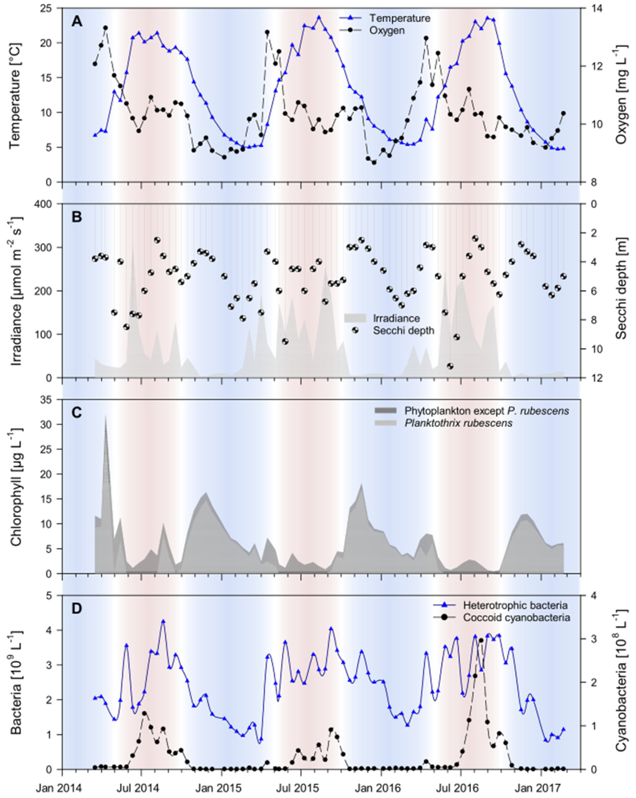
3.1. Seasonal Dynamics of Environmental Parameters

Throughout the three-year sampling campaign of our study, the environmental parameters in the epilimnion of Lake Zurich displayed re-occurring seasonal patterns (Figure 1, Table S1). These patterns allowed for distinguishing one season characterized by cold water temperature lasting from October to April, and one season characterized by warm water temperatures lasting from May to September. Although irradiance by sunlight was naturally higher in the warm season, chlorophyll concentrations and Secchi depths were lowest, which is a clear indication that phytoplankton could not establish stable populations. Planktothrix rubescens-related phycoerythrin contributed only a small portion to the total chlorophyll concentration, while heterotrophic bacteria and coccoid cyanobacteria thrived during warm season conditions. By contrast, irradiance was low in the cold season, but total chlorophyll concentrations more than doubled because of massive increases of phycoerythrin-containing P. rubescens. These increases also led to less transparency of epilimnetic waters as documented by smaller Secchi depths. Unlike P. rubescens, heterotrophic bacteria and coccoid cyanobacteria reached their respective minima in the cold season.

3.2. Co-Occurrence Network Properties

Two distinct seasonal groups emerged from non-metric multidimensional scaling (NMDS) of the epilimnetic protistan plankton time-series metabarcoding data of Lake Zurich (Figure 2). One group consisted of cold season communities sampled between October to April. The other group consisted of warm-season communities sampled between May and September. A third seasonal group, which comprised distinctive spring sample communities could not be observed. According to this pattern, we split the complete metabarcoding dataset into one cold season dataset and one warm season dataset and ran independent co-occurrence network analyses for each of the two seasons. The size of the input datasets was similar for both seasons, with slightly more samples but fewer network sequence clusters (NSCs; operational taxonomic units that resulted from two-level sequence clustering) in the cold season dataset (Table 2). Likewise, the size of the resulting networks was similar, however, with slightly more NSCs (nodes) but distinctively fewer associations (edges) in the warm season. The threshold values for Spearman’s rho differed only marginally between the cold season (−0.59 and 0.60) and the warm season dataset (−0.61 and 0.62). Although some negative correlations were observed, none of them passed the statistically determined thresholds for significant co-exclusions between NSCs. Thus, all edges in the networks represent co-occurrences between NSCs. All other network properties pointed towards a more complex network structure in the cold season plankton community. Even though fewer nodes were found in the cold season network, they were connected by notably more edges (6872 edges linking 946 nodes; Figure 3A) compared to the warm season network (5252 edges linking 973 nodes; Figure 3B). This finding is corroborated by a higher ratio of realized three-way associations (transitivity) and a higher ratio of total realized associations (density) between protists in the cold season community. In contrast, the lower complexity of the warm season network can be inferred from a longer average path distance, lower average degree, and a larger diameter. All three observations indicate a warm-season protistan plankton community in which associations between community members were not as frequently observed and in which the network structure was therefore not as tight as in the cold season community. Finally, of 68 connected components in the warm season network, 61 consisted of only one pair of NSCs. This is a further indication that the warm season community was more partitioned than its cold season counterpart, which is expressed by a higher modularity of the former network.
A targeted removal of nodes with the highest betweenness centrality from the cold season network led to a gradual loss of connectivity at the beginning of a species extinction scenario (up to 13% loss after removing 30 nodes, Figure 4). The buffering capacity of the cold season community becomes compromised after the removal of the top 31 nodes with the highest betweenness. When these nodes were removed, the loss of connectivity was 51%. A total breakdown of the cold season community network (loss of 95% of the connectivity) was observed after the removal of the top 192 nodes with the highest betweenness values. The warm season network was more vulnerable and less robust towards species extinction (Figure 4). A first clear negative effect on the buffering capacity of the community was observed after removing the top 17 nodes with the highest betweenness (loss of connectivity reaching 17%). After the removal of the top 31 nodes with the highest betweenness centrality, the loss of connectivity increased to 48%. The total breakdown of community network structures in the warm season (loss of 95% of the connectivity), was already achieved notably sooner compared to the cold season network, namely after the removal of the top 162 nodes with the highest betweenness.

3.3. Impact of Environmental Parameters on the Co-Occurrence Networks

The separation of the epilimnion time-series samples into one cold season and one warm season dataset was further supported by the seasonal dynamics of environmental parameters in Lake Zurich (Figure 1, Table S1). Eleven environmental parameters correlated with NSCs in the cold season network (Figure 3A; ordered in decreasing number of significant correlations to NSCs): bacterial abundance, water temperature, conductivity, oxygen saturation, Secchi depth, coccoid cyanobacterial abundance, oxygen concentration, Planktothrix rubescens-related chlorophyll concentration, total chlorophyll concentration, irradiance, and bacteria with high nucleic acid content. In contrast, only five environmental parameters correlated with NSCs in the warm season network (Figure 3B; ordered in decreasing number of significant correlations to NSCs): water temperature, coccoid cyanobacterial abundance, oxygen saturation, diatom-related chlorophyll concentration, and conductivity. All parameters that appeared in both networks shared a higher number of correlations with NSCs in the cold season than in the warm season (Table S2). This observation from within network structures translates into the following biological result: a larger fraction of protists is adapted to Lake Zurich’s environmental conditions in the cold season water phase than to those in the warm season water phase.

3.4. Taxonomic Composition of the Co-Occurrence Networks

Despite different network properties, the community composition within the networks of both seasons was similar on higher taxonomic levels. The two most diverse taxon groups in the cold season (Figure 5A) were Stramenopiles (319 NSCs) and Alveolata (256 NSCs). Within the Stramenopiles, Chrysophyceae were represented with the highest number of NSCs (n = 150), while diatoms (Bacillariophyta) played only a minor role (14 NSCs). Ciliophora (120 NSCs) was the most diverse phylum within the Alveolata, closely followed by Dinoflagellata (115 NSCs). Similarly, the two most diverse taxon groups in the warm season (Figure 5B) were also Stramenopiles (341 NSCs) and Alveolata (237 NSCs). Within the Stramenopiles, the Chrysophyceae were similarly diverse as in the cold season network (155 NSCs). The diversity of diatoms, however, increased to 27 NSCs. Likewise, the amount of alveolate NSCs remained similar compared to the cold season, with Ciliophora reaching 109 NSCs and Dinoflagellata 108 NSCs. A notable increase of NSCs from cold to warm-season was observed for Fungi (from 51 NSCs to 80 NSCs) and Chlorophyta (from 31 NSCs to 59 NSCs).
A considerable number of 531 NSCs were shared between the two seasonal networks. The NSCs that occurred simultaneously in both networks throughout the year belonged mainly to Stramenopiles (205 NSCs), Alveolata (120 NSCs), Opisthokonta (67 NSCs; including Fungi), Rhizaria (56 NSCs), and Cryptista (40 NSCs). Among these taxonomic groups, most NSCs shared by both networks were further affiliated to Chrysophyceae (81 NSCs) and Ciliophora (76 NSCs).

3.5. Key Nodes of the Co-Occurrence Networks

Measures from graph theory allowed for defining 56 key nodes in the protistan plankton community network of the cold season and 46 key nodes in the network of the warm season (Figure 5C,D). The most abundant taxon groups among key nodes in the cold season were Alveolata (22 NSCs, of which 13 belonged to ciliates) and Stramenopiles (19 NSCs, of which 9 belonged to chrysophytes). Similarly, the most abundant taxon groups among key nodes in the warm season were also Alveolata (16 key nodes, of which 12 belonged to ciliates) and Stramenopiles (16 key nodes, of which 7 belonged to chrysophytes). Five taxonomic key nodes were shared between the two seasonal networks, which were Nannochloropsis limnetica (Stramenopiles), Cryptomonas curvata (Cryptista), and three ciliates (Euplotidae, Halteria sp., Halteriidae). One further shared key node was an environmental parameter (conductivity).
As an example, the two subnetworks of Halteria sp., one of the five shared taxonomic key nodes in both networks, were further investigated. The biological associations of this key node taxon were remarkably distinct in a comparison of both seasonal networks. In the cold season, Halteria sp. was associated with 36 significantly correlating nodes (Figure 6A). Most of these nodes were assigned to other ciliate species (e.g., Histiobalantium sp. or Askenasia sp.) and Chrysophyceae (e.g., Dinobryon bavaricum, Dinobryon sociale, and Uroglena americanum) commonly found in freshwater habitats. Furthermore, we found indications that Halteria sp. is a species linking different trophic levels, since it was co-occurring with Mesocyclops sp. (possibly Mesocyclops leuckarti, a frequent copepod in Lake Zurich) and correlating with the abundance of coccoid cyanobacteria. In the warm season network, Halteria sp. was associated with only eight significantly correlating partners, most of which were assigned to the Stramenopiles genus Pedinella (Figure 6B). In the cold season, Halteria sp. was co-occurring with Pedinella less frequently. The comparison of Halteria sp.’s subnetworks of the cold and warm season showed that members of similar taxonomic groups co-occurred with this ciliate key node, though the warm season subnetwork was conspicuously reduced compared to its counterpart of the cold season.

4. Discussion

4.1. Placing Co-Occurrence Networks into Perspective

Although co-occurrence network analyses are limited to deriving potential species association patterns exclusively from significant correlations in species (or ASV, OTU) abundance matrices rather than from experimental observations, numerous studies have shown that such associations can be correctly predicted. More importantly, they allow for drawing valuable conclusions on community- or ecosystem-level [12,14,17,18,19,22,23,24,43]. The success and reliability of such studies, however, strongly depend on the quality of the network analysis design. Therefore, we here used state-of-the-art knowledge and methodologies to consider the critical points in co-occurrence network analyses [28,72,73]. To mention some examples: (i) the analyses of this study were based on abundance profiles obtained from time-series metabarcoding instead of mere presence-absence data [72]. (ii) Highly similar sequences placed in multiple OTUs were agglomerated by a second-level clustering strategy. This diminished excessive false-positive co-occurrences of nodes and edges that actually represented an intraspecific genetic variation of the same organism or species [19,59]. (iii) The actual assessment of significant correlations employed a null model approach [16], which was identified as a positive exception in critical reviews of ecological network analyses [72,73]. Nevertheless, we point out that eventually, conclusions drawn from network analyses require rigorous testing in specifically designed experimental studies with e.g., cultivated species, or with targeted observations in natural systems. Network analyses provide, thus, the hypothesis framework to build explanatory models and fuel further research [19,73].

4.2. Succession in the Protistan Plankton Network of Lake Zurich Is Affected by Climate Change

Seasonal succession of microbial eukaryote communities is well documented and has been studied in many lake ecosystems [7,11,74]. Our time-series metabarcoding approach confirms previously reported patterns of distinct protistan plankton communities in the cold and warm season [3,4,75,76] and the absence of phytoplankton spring blooms from the epilimnion in Lake Zurich [77]. These observed succession patterns are largely the result of seasonally changing physicochemical parameters (Figure 1, Figure 4 and Figure S1, Table S1) that have been drastically altered by global warming during the last decades [45,46,47,48,49]. By inferring the protistan co-occurrence network of each season, we revealed consequences for succession patterns of a model lake ecosystem subjected to climate change. Previous studies [45,47] demonstrated that while environmental stress in Lake Zurich often originates in autumn and winter (corroborating with the cold season dataset of our study), the consequences for plankton communities are most severe in spring and summer (corroborating with the warm season dataset of our study). Especially lake water surface temperatures significantly increased in the wake of climate change [46]. This process of lake warming is further accelerated by significantly increased air temperatures in spring [46] and has led to drastic changes in the stratification regime that prevents complete water turnovers in Lake Zurich. The strong impact of water temperature as a major stressor in Lake Zurich can be derived from its position in both networks, from which it emerged as the environmental parameter with most correlations to protists (Table S2). Further time-lagged consequences caused by the effect of water temperature on the lake ecosystem are evident in the networks from the roles of eukaryotic phytoplankton organisms and of Planktothrix rubescens, a filamentous cyanobacterium able to form massive blooms [78]. Thermocline-induced incomplete water turnovers resulted in a nutrient depletion in the epilimnion of Lake Zurich during our investigation period (2014–2017; see Table 1 and Yankova et al. [45]). Unlike most eukaryotic phytoplankton organisms, P. rubescens is capable of living in phosphorus-poor environments and is, therefore, the major profiteer of climate change in Lake Zurich [47]. In the warm season, however, P. rubescens descends into the metalimnion (10–15 m depths) [78] and is not directly associated with protists in epilimnetic communities. According to this chain of cause and effect, protistan phytoplankton does not find adequate environmental prerequisites to play major roles in the networks of both seasons (with little increase in the warm season compared to the cold season; Figure 5), while several protists significantly correlated with the opportunistic P. rubescens in the cold season, but none in the warm season (Table S2).
The identification of water temperature as a major determinant associated with numerous protistan taxa especially in the cold season underlines its influence on co-occurrence patterns among protists in the epilimnion. Also, the effects of other environmental parameters triggered by lake warming became obvious as they significantly correlated with protistan co-occurrence patterns. These parameters include for example oxygen (both saturation and concentration), which was linked to a different set of organisms in either season, which suggests that this parameter is one of the most important environmental variables associated with planktonic organisms in the epilimnion of Lake Zurich. Even though the epilimnion in Lake Zurich was saturated with oxygen in the warm season, a simultaneous decrease in conductivity indicated fewer solutes and nutrients in the epilimnion during this time of the year. Consequently, fewer protists correlated with conductivity measures in the warm than in the cold season, when more solutes were available.
Throughout the time of lake warming in Lake Zurich, phytoplankton communities have not been able to recover or to adapt to the new environmental conditions, as evident from the continuous non-initiation of spring blooms. Thus, the phytoplankton community is neither able to resist the ecosystem disturbance induced by climate change nor to recover to a stable state during the three-year observation cycle of this study. This suggests that both ecosystem robustness and resilience in Lake Zurich are compromised. Considering that lake warming in Lake Zurich is unlikely to cease soon, it is not possible to project the evolution of phytoplankton communities and the adaptation of the ecosystem to a steady state. Previous reports showed that the phytoplankton spring bloom could at least partly recover in cooler years because complete water turnover was restored in Lake Zurich [45]. But such occasions were not recorded in the three-year sampling campaign of our study.

4.3. Ecological Consequences for Different Protist Groups Inferred from Climate-Stressed Networks

The Plankton Ecology Group (PEG) model predicts two distinct peaks of protistan phytoplankton and zooplankton in spring and summer for eutrophic and mesotrophic lakes [4]. Protistan plankton succession in Lake Zurich had established such peaks for decades [77], but recent environmental changes have resulted in a surplus re-oligotrophication of the lake and an absence of characteristic epilimnetic spring bloom communities that used to be formed by autotrophic cryptophytes and diatoms [45,47]. Instead of matching the predictions of the PEG model for eutrophic and mesotrophic lakes, the succession patterns of protistan plankton in Lake Zurich have thus started to follow the predictions for a typical oligotrophic lake with a small or no abundance peak in spring and a second small peak in late summer [4]. The community structure inferred from our network analyses confirmed Lake Zurich’s transformation to an oligotrophic state, with the notable exception that the diminished role of protistan phytoplankton did not meet the expectations of the PEG model (Figure 5). This was most pronounced in the warm season network when many autotrophic protists were associated with Chytridiomycota is known to parasitize algae [79,80]. The stress-induced by climate change might make autotrophic organisms more susceptible to parasitism [81], and the combination of abiotic and biotic stressors might cumulate in an amplification of phytoplankton decline.
The climate-stress-induced decline of phytoplankton results in multiple consequences for the protistan plankton community networks. Most of all for heterotrophic protists such as ciliates, which are the main predators of protistan phytoplankton in oligotrophic lakes [4]. With autotrophs largely missing from the protistan plankton network, ciliates are forced to expand their prey spectrum towards other organisms. The co-occurrence networks indicate that nanoflagellates might fill this vacancy as by far the most associations were observed between ciliates and chrysophytes. This finding contrasts results from previous co-occurrence networks between ciliates and other planktonic organisms in Lake Zurich when phytoplankton spring blooms are successfully established [82]. In these networks, associations between chrysophytes and ciliates had not outnumbered associations between phytoplankton (especially diatoms) and ciliates. Indeed, ciliates feed on chrysophytes [83,84] and many associations may indicate predator-prey relationships. With the decline of autotrophic phytoplankton as their preferred food source, chrysophytes might become the ciliates’ most important prey throughout the year in the protistan plankton community network. However, not all associations in the networks between these two groups necessarily reflect predator-prey relations. Especially in winter, some associations may indicate an overlap in feeding strategies, because both ciliates and chrysophytes comprise effective bacterivores [85] and share the same food source (i.e., bacteria) with which they are both co-occurring. Alternatively, the significant co-occurrences between ciliates and chrysophytes could indicate a preference towards similar environmental conditions.
Moreover, ciliates emerged as the most important taxon group from the networks for mediating processes that affected a majority of other organisms (see betweenness results in Figure 5C,D). Thereby, the relation of ciliates to other organisms was either direct or indirect, when ciliates connected two other nodes which were not directly connected themselves. An example for such a three-way association can be found in the cold season subnetwork of Halteria sp., which correlated with coccoid cyanobacteria and simultaneously with a crustacean Mesocyclops species (Figure 6A). This result illustrates the potential role of ciliates in linking energy fluxes between different trophic levels [1]. Results from a morphological study characterized Halteria grandinella as a major bacterivore in freshwater food webs which corroborates well with our identification of Halteria sp. as a key species in the protistan plankton community network [85]. Likewise, ciliates of the genus Halteria are known for their characteristic jumping behavior that is a strategy to escape zooplankton predators such as rotifers or copepods to which Mesocyclops belongs [86,87,88]. The example of Halteria sp. illustrates how autecological knowledge of species corroborates findings of co-occurrence network analyses. In this particular case, we, based on ecological knowledge of this species, find a confirmation of the statistically derived associations in the network (Halteria sp. as a keystone species functioning as an important trophic link).
Apart from affecting ciliate feeding behavior, phytoplankton decline in the networks also enhanced the role of mixotrophic chrysophyte taxa, such as Dinobryon and Ochromonas, which can perform photosynthesis in addition to feeding on bacteria [89,90]. This versatile lifestyle gives them an advantage over obligate autotrophic protists in Lake Zurich that are depending on favorable light conditions and the availability of nutrients. In the cold season, mixotrophs can meet their energy demand by using bacteria as a primary energy source. In the warm season, the energy demand of mixotrophs can be covered by performing photosynthesis even under nutrient shortage. Mixotrophic chrysophytes might continue to feed on bacteria at low rates in the warm season to ensure that their energy demand is covered. However, statistically significant correlations between mixotrophic chrysophytes and bacteria were only observed in the cold season and not in the warm season network. Therefore, this scenario needs further testing in lab experiments.

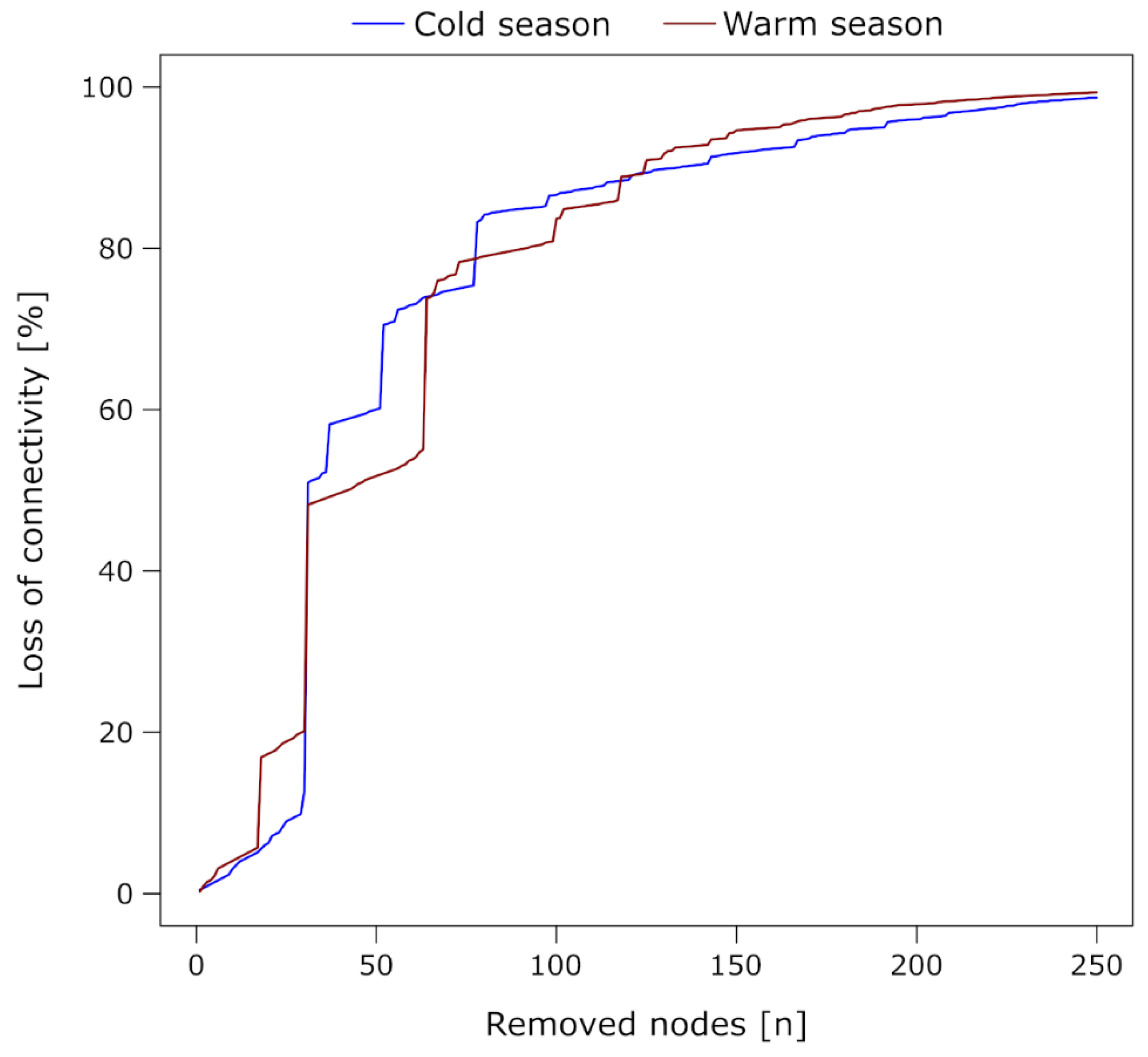
4.4. Assessing Ecosystem Resilience of Lake Zurich with Protistan Community Networks

Our results showed that biotic and abiotic associations within protistan plankton communities in Lake Zurich are more complex and more robust towards disturbances in the cold compared to the warm season (Table 2, Figure 3 and Figure 4). Thereby, the climate-change-induced stress in Lake Zurich can be categorized as a press disturbance [15], since it has been continuously affecting the ecosystem for years (and will continue to do so). A study of vertebrate communities in terrestrial ecosystems illustrated how network analyses of complex co-occurrence patterns among species can assess the impact of climate change on ecosystems [27]. Based on their results, the authors developed a framework in which robustness and connectivity emerged as indicative network metrics for the susceptibility of an ecological community to climate change. Studies on bacteria [23,24,26,37], marine communities [42,43], and benthic macroinvertebrates [91] have successfully applied similar strategies for inferring the effect of environmental stressors from network analyses of community data. Different indicator measures exist for assessing the complexity of a co-occurrence network based on metabarcoding data [12]. Our results (Table 2) demonstrate that a larger input dataset does not necessarily lead to a network that comprises more nodes (here protists) and edges (here co-occurrences). Neither does a count of nodes or edges alone allow for concluding the complexity of a network. Such conclusions need to be drawn from the network topology, by putting the numbers of nodes and edges into context and inferring their distribution and connection patterns within the network. The density of a network is one such metric and displays how many of the potential edges (with regard to the total number of nodes) are effectively established. The higher the density, the more associations in the network, and the more complex and resilient to stressors the community network become [92,93]. Average path length, average degree, and diameter are indirectly linked to density and also evaluate the distribution of edges in a network. With more associations established among the same number of organisms in a network, mean path distance and diameter decrease, and the complexity of the network increases. Another indicator measure for the complexity of a network is modularity. If this measure is high, the network is partitioned into many groups in which protists are co-occurring with each other but less with nodes from other groups (similar to functional guilds) and the network complexity decreases. Although modularity was just marginally higher in the warm season protistan plankton community network of Lake Zurich, the lower level of complexity in the warm season can further be derived from the partitioning of its co-occurrence network into many more connected components (most of which consisting of only two nodes) than in the cold season co-occurrence network.
Since functional redundancy correlates with ecosystem resilience [94], we referred to network transitivity as an indicator measure for inferring functional redundancy in the protistan plankton community networks. This metric indicates redundant associations, by measuring the probability that two nodes are at the same time, directly and indirectly, connected [12]. The higher this probability, the more redundant are associations in the network and the more complex and robust towards the extinction of species becomes the protistan community. Finally, we also assessed ecosystem resilience by documenting the response of the network towards targeted attacks (Figure 4). The longer a community network can maintain its structure and buffer the loss of connectivity, the more robust and less vulnerable it is. Thereby, functional redundancy has a positive effect on network robustness, because of its buffering capacity on node removal from the network.
Ongoing climate change can accelerate the loss of ecosystem resilience by promoting changes in protistan plankton community networks. However, it is currently difficult to predict whether the changes will continue towards a collapse of the networks or whether they lead to another stable state with permanent changes in ecosystem function and services. The latter assumption finds support in reports about declining fish stocks and increased costs for drinking water purification [95,96]. Beyond large-scale consequences for ecosystems, co-occurrence networks obtained from large metabarcoding datasets proved beneficial for developing hypotheses about autecological species-specific relationships. Based on these hypotheses, future interdisciplinary approaches can be designed where limnology, ecology, and molecular as well as morphological taxonomic expertise are considered to elucidate specific key players and their function in aquatic microbial food webs.

Supplementary Materials

The following are available online at https://0-www-mdpi-com.brum.beds.ac.uk/2076-2607/9/3/549/s1, Table S1: Time-series data of environmental parameters, Table S2: Network properties of environmental parameter nodes in both seasons, Figure S1: NMDS of environmental parameter time-series data.

Author Contributions

Conceptualization, B.S., T.P. (Thomas Posch), T.S., and D.F.; methodology—field sampling and environmental parameters, G.P., E.P.B., B.K., T.P. (Thomas Pröschold), B.S., and T.P. (Thomas Posch); methodology—molecular analyses, Z.Q.; software and formal analysis, D.F; investigation, B.S., T.P. (Thomas Posch), T.S., and D.F.; writing—original draft preparation, T.S. and D.F.; writing—review & editing, B.S. and T.P. (Thomas Posch); funding acquisition, B.S., T.P. (Thomas Posch), and T.S. All authors have read and agreed to the final version of the manuscript.

Funding

This study was supported by the Swiss National Science Foundation (SNF; projects SNF 31003A-182489 and SNF 310030E-160603), the Austrian Science Fund (FWF; project I2238-B25), the German Research Foundation (DFG; project STO 414/13-1), and a research grant by the Carl-Zeiss Foundation to D.F.

Data Availability Statement

The data presented in this study are openly available at the Sequence Read Archive of the National Center for Biotechnology Information (NCBI) under project number PRJNA609412.

Acknowledgments

We thank the captains Eugen Loher and Daniel Marty for help during sampling campaigns and the Water Supply Company Zurich for support with measuring environmental parameters.

Conflicts of Interest

The authors declare no conflict of interest.

References

  1. Sherr, B.F.; Sherr, E.B.; Hopkinson, C.S. Trophic Interactions within Pelagic Microbial Communities: Indications of feedback regulation of carbon flow. Hydrobiologia 1988, 159, 19–26. [Google Scholar] [CrossRef]
  2. Stockner, J.G.; Porter, K.G. Microbial food webs in freshwater planktonic ecosystems. In Complex Interactions in Lake Communities; Carpenter, S.R., Ed.; Springer: New York, NY, USA, 1988; pp. 69–83. ISBN 978-1-4612-3838-6. [Google Scholar]
  3. Sommer, U.; Gliwicz, Z.M.; Lampert, W.; Duncan, A. The PEG-model of seasonal succession of planktonic events in fresh waters. Arch. Hydrobiol. 1986, 106, 433–471. [Google Scholar]
  4. Sommer, U.; Adrian, R.; de Senerpont Domis, L.; Elser, J.J.; Gaedke, U.; Ibelings, B.; Jeppesen, E.; Lürling, M.; Molinero, J.C.; Mooij, W.M.; et al. Beyond the Plankton Ecology Group (PEG) Model: Mechanisms driving plankton succession. Annu. Rev. Ecol. Evol. Syst. 2012, 43, 429–448. [Google Scholar] [CrossRef]
  5. Giner, C.R.; Balagué, V.; Krabberød, A.K.; Ferrera, I.; Reñé, A.; Garcés, E.; Gasol, J.M.; Logares, R.; Massana, R. Quantifying long-term recurrence in planktonic microbial eukaryotes. Mol. Ecol. 2019, 28, 923–935. [Google Scholar] [CrossRef] [PubMed]
  6. Lallias, D.; Hiddink, J.G.; Fonseca, V.G.; Gaspar, J.M.; Sung, W.; Neill, S.P.; Barnes, N.; Ferrero, T.; Hall, N.; Lambshead, P.J.D.; et al. Environmental metabarcoding reveals heterogeneous drivers of microbial eukaryote diversity in contrasting estuarine ecosystems. ISME J. 2015, 9, 1208–1221. [Google Scholar] [CrossRef] [PubMed]
  7. Lemke, M.J.; Paver, S.F.; Dungey, K.E.; Velho, L.F.M.; Kent, A.D.; Rodrigues, L.C.; Kellerhals, D.M.; Randle, M.R. Diversity and succession of pelagic microorganism communities in a newly restored Illinois River Floodplain Lake. Hydrobiologia 2017, 804, 35–58. [Google Scholar] [CrossRef] [Green Version]
  8. Chonova, T.; Kurmayer, R.; Rimet, F.; Labanowski, J.; Vasselon, V.; Keck, F.; Illmer, P.; Bouchez, A. Benthic diatom communities in an alpine river impacted by waste water treatment effluents as revealed using DNA metabarcoding. Front. Microbiol. 2019, 10, 653. [Google Scholar] [CrossRef] [PubMed]
  9. Moreira, D.; López-García, P. Time series are critical to understand microbial plankton diversity and ecology. Mol. Ecol. 2019, 28, 920–922. [Google Scholar] [CrossRef] [PubMed]
  10. Nolte, V.; Pandey, R.V.; Jost, S.; Medinger, R.; Ottenwälder, B.; Boenigk, J.; Schlötterer, C. Contrasting seasonal niche separation between rare and abundant taxa conceals the extent of protist diversity. Mol. Ecol. 2010, 19, 2908–2915. [Google Scholar] [CrossRef] [PubMed] [Green Version]
  11. Simon, M.; López-García, P.; Deschamps, P.; Moreira, D.; Restoux, G.; Bertolino, P.; Jardillier, L. Marked seasonality and high spatial variability of protist communities in shallow freshwater systems. ISME J. 2015, 9, 1941–1953. [Google Scholar] [CrossRef] [Green Version]
  12. Karimi, B.; Maron, P.A.; Chemidlin-Prevost Boure, N.; Bernard, N.; Gilbert, D.; Ranjard, L. Microbial diversity and ecological networks as indicators of environmental quality. Environ. Chem. Lett. 2017, 15, 265–281. [Google Scholar] [CrossRef]
  13. Allison, S.D.; Martiny, J.B.H. Resistance, resilience, and redundancy in microbial communities. Proc. Natl. Acad. Sci. USA 2008, 105, 11512–11519. [Google Scholar] [CrossRef] [Green Version]
  14. Naylor, D.; Sadler, N.; Bhattacharjee, A.; Graham, E.B.; Anderton, C.R.; McClure, R.; Lipton, M.; Hofmockel, K.S.; Jansson, J.K. Soil microbiomes under climate change and implications for carbon cycling. Annu. Rev. Environ. Resour. 2020, 45, 29–59. [Google Scholar] [CrossRef]
  15. Shade, A.; Peter, H.; Allison, S.D.; Baho, D.; Berga, M.; Buergmann, H.; Huber, D.H.; Langenheder, S.; Lennon, J.T.; Martiny, J.B.; et al. Fundamentals of microbial community resistance and resilience. Front. Microbiol. 2012, 3, 417. [Google Scholar] [CrossRef] [PubMed] [Green Version]
  16. Connor, N.; Barberán, A.; Clauset, A. Using null models to infer microbial co-occurrence networks. PLoS ONE 2017, 12, e0176751. [Google Scholar] [CrossRef] [Green Version]
  17. Faust, K.; Lahti, L.; Gonze, D.; de Vos, W.M.; Raes, J. Metagenomics meets time series analysis: Unraveling microbial community dynamics. Curr. Opin. Microbiol. 2015, 25, 56–66. [Google Scholar] [CrossRef] [Green Version]
  18. Faust, K.; Raes, J. Microbial interactions: From networks to models. Nat. Rev. Microbiol. 2012, 10, 538–550. [Google Scholar] [CrossRef]
  19. Röttjers, L.; Faust, K. From hairballs to hypotheses–biological insights from microbial networks. FEMS Microbiol. Rev. 2018, 42, 761–780. [Google Scholar] [CrossRef] [Green Version]
  20. Weiss, S.; Treuren, W.V.; Lozupone, C.; Faust, K.; Friedman, J.; Deng, Y.; Xia, L.C.; Xu, Z.Z.; Ursell, L.; Alm, E.J.; et al. Correlation detection strategies in microbial data sets vary widely in sensitivity and precision. ISME J. 2016, 10, 1669–1681. [Google Scholar] [CrossRef] [PubMed]
  21. Fuhrman, J.A.; Cram, J.A.; Needham, D.M. Marine microbial community dynamics and their ecological interpretation. Nat. Rev. Microbiol. 2015, 13, 133–146. [Google Scholar] [CrossRef] [PubMed]
  22. Vacher, C.; Tamaddoni-Nezhad, A.; Kamenova, S.; Peyrard, N.; Moalic, Y.; Sabbadin, R.; Schwaller, L.; Chiquet, J.; Smith, M.A.; Vallance, J.; et al. Chapter one-learning ecological networks from next-generation sequencing data. In Ecosystem Services: From Biodiversity to Society, Part 2. Advances in Ecological Research; Woodward, G., Bohan, D.A., Eds.; Academic Press: Cambridge, MA, USA, 2016; Volume 54, pp. 1–39. [Google Scholar]
  23. Mandakovic, D.; Rojas, C.; Maldonado, J.; Latorre, M.; Travisany, D.; Delage, E.; Bihouée, A.; Jean, G.; Díaz, F.P.; Fernández-Gómez, B.; et al. Structure and co-occurrence patterns in microbial communities under acute environmental stress reveal ecological factors fostering resilience. Sci. Rep. 2018, 8, 5875. [Google Scholar] [CrossRef]
  24. De Vries, F.T.; Griffiths, R.I.; Bailey, M.; Craig, H.; Girlanda, M.; Gweon, H.S.; Hallin, S.; Kaisermann, A.; Keith, A.M.; Kretzschmar, M.; et al. Soil bacterial networks are less stable under drought than fungal networks. Nat. Commun. 2018, 9, 3033. [Google Scholar] [CrossRef] [Green Version]
  25. Evans, D.M.; Kitson, J.J.N.; Lunt, D.H.; Straw, N.A.; Pocock, M.J.O. Merging DNA metabarcoding and ecological network analysis to understand and build resilient terrestrial ecosystems. Funct. Ecol. 2016, 30, 1904–1916. [Google Scholar] [CrossRef] [Green Version]
  26. Wang, Y.; Zhang, R.; Zheng, Q.; Deng, Y.; van Nostrand, J.D.; Zhou, J.; Jiao, N. Bacterioplankton community resilience to ocean acidification: Evidence from microbial network analysis. ICES J. Mar. Sci. 2016, 73, 865–875. [Google Scholar] [CrossRef]
  27. Araújo, M.B.; Rozenfeld, A.; Rahbek, C.; Marquet, P.A. Using species co-occurrence networks to assess the impacts of climate change. Ecography 2011, 34, 897–908. [Google Scholar] [CrossRef]
  28. Berry, D.; Widder, S. Deciphering microbial interactions and detecting keystone species with co-occurrence networks. Front. Microbiol. 2014, 5, 219. [Google Scholar] [CrossRef] [Green Version]
  29. Banerjee, S.; Schlaeppi, K.; van der Heijden, M.G.A. Keystone taxa as drivers of microbiome structure and functioning. Nat. Rev. Microbiol. 2018, 16, 567–576. [Google Scholar] [CrossRef] [PubMed]
  30. Tian, L.; Bashan, A.; Shi, D.-N.; Liu, Y.-Y. Articulation points in complex networks. Nat. Commun. 2017, 8, 1–9. [Google Scholar] [CrossRef] [Green Version]
  31. Clauset, A.; Newman, M.E.J.; Moore, C. Finding community structure in very large networks. Phys. Rev. E 2004, 70, 066111. [Google Scholar] [CrossRef] [Green Version]
  32. Blondel, V.D.; Guillaume, J.-L.; Lambiotte, R.; Lefebvre, E. Fast unfolding of communities in large networks. J. Stat. Mech. 2008, 10, P10008. [Google Scholar] [CrossRef] [Green Version]
  33. Chaffron, S.; Rehrauer, H.; Pernthaler, J.; von Mering, C. A Global network of coexisting microbes from environmental and whole-genome sequence data. Genome Res. 2010, 20, 947–959. [Google Scholar] [CrossRef] [PubMed] [Green Version]
  34. Freilich, M.A.; Wieters, E.; Broitman, B.R.; Marquet, P.A.; Navarrete, S.A. Species co-occurrence networks: Can they reveal trophic and non-trophic interactions in ecological communities? Ecology 2018, 99, 690–699. [Google Scholar] [CrossRef] [PubMed]
  35. Dini-Andreote, F.; de Cássia Pereira e Silva, M.; Triadó-Margarit, X.; Casamayor, E.O.; van Elsas, J.D.; Salles, J.F. Dynamics of bacterial community succession in a salt marsh chronosequence: Evidences for Temporal niche partitioning. ISME J. 2014, 8, 1989–2001. [Google Scholar] [CrossRef] [PubMed] [Green Version]
  36. Faust, K.; Lima-Mendez, G.; Lerat, J.-S.; Sathirapongsasuti, J.F.; Knight, R.; Huttenhower, C.; Lenaerts, T.; Raes, J. Cross-Biome comparison of microbial association networks. Front. Microbiol. 2015, 6, 1200. [Google Scholar] [CrossRef] [Green Version]
  37. Peura, S.; Bertilsson, S.; Jones, R.I.; Eiler, A. Resistant microbial cooccurrence patterns inferred by network topology. Appl. Environ. Microbiol. 2015, 81, 2090–2097. [Google Scholar] [CrossRef] [Green Version]
  38. Albert, R.; Jeong, H.; Barabási, A.-L. Error and attack tolerance of complex networks. Nature 2000, 406, 378–382. [Google Scholar] [CrossRef] [Green Version]
  39. Holme, P.; Kim, B.J.; Yoon, C.N.; Han, S.K. Attack vulnerability of complex networks. Phys. Rev. E 2002, 65, 056109. [Google Scholar] [CrossRef] [PubMed] [Green Version]
  40. Klau, G.W.; Weiskircher, R. Robustness and resilience. In Network Analysis; Brandes, U., Erlebach, T., Eds.; Springer: Berlin/Heidelberg, Germany, 2005; pp. 417–437. ISBN 978-3-540-31955-9. [Google Scholar]
  41. Gao, J.; Barzel, B.; Barabási, A.-L. Universal resilience patterns in complex networks. Nature 2016, 530, 307–312. [Google Scholar] [CrossRef]
  42. Kéfi, S.; Miele, V.; Wieters, E.A.; Navarrete, S.A.; Berlow, E.L. How structured is the entangled bank? The surprisingly simple organization of multiplex ecological networks leads to increased persistence and resilience. PLoS Biol. 2016, 14, e1002527. [Google Scholar] [CrossRef]
  43. Needham, D.M.; Sachdeva, R.; Fuhrman, J.A. Ecological dynamics and co-occurrence among marine phytoplankton, bacteria and myoviruses shows microdiversity matters. ISME J. 2017, 11, 1614–1629. [Google Scholar] [CrossRef] [PubMed] [Green Version]
  44. Lupatini, M.; Suleiman, A.K.A.; Jacques, R.J.S.; Antoniolli, Z.I.; de Siqueira Ferreira, A.; Kuramae, E.E.; Roesch, L.F.W. Network topology reveals high connectance levels and few key microbial genera within soils. Front. Environ. Sci. 2014, 2, 10. [Google Scholar] [CrossRef] [Green Version]
  45. Yankova, Y.; Neuenschwander, S.; Köster, O.; Posch, T. Abrupt stop of deep water turnover with lake warming: drastic consequences for algal primary producers. Sci. Rep. 2017, 7, 1–9. [Google Scholar] [CrossRef] [PubMed] [Green Version]
  46. Yankova, Y.; Villiger, J.; Pernthaler, J.; Schanz, F.; Posch, T. Prolongation, deepening and warming of the metalimnion change habitat conditions of the harmful Filamentous Cyanobacterium Planktothrix Rubescens in a prealpine lake. Hydrobiologia 2016, 776, 125–138. [Google Scholar] [CrossRef] [Green Version]
  47. Posch, T.; Köster, O.; Salcher, M.M.; Pernthaler, J. Harmful Filamentous Cyanobacteria favoured by reduced water turnover with lake warming. Nat. Clim. Chang. 2012, 2, 809–813. [Google Scholar] [CrossRef] [Green Version]
  48. Livingstone, D.M. Impact of secular climate change on the thermal structure of a large temperate central european lake. Clim. Chang. 2003, 57, 205–225. [Google Scholar] [CrossRef]
  49. North, R.P.; North, R.L.; Livingstone, D.M.; Köster, O.; Kipfer, R. Long-term changes in hypoxia and soluble reactive phosphorus in the hypolimnion of a large temperate lake: Consequences of a climate regime shift. Glob. Chang. Biol. 2014, 20, 811–823. [Google Scholar] [CrossRef] [PubMed]
  50. Qu, Z.; Forster, D.; Bruni, E.P.; Frantal, D.; Kammerlander, B.; Nachbaur, L.; Pitsch, G.; Posch, T.; Pröschold, T.; Teubner, K.; et al. Aquatic food webs in deep temperate lakes: key species establish through their autecological versatility. Mol. Ecol. 2021, 30, 1053–1071. [Google Scholar] [CrossRef] [PubMed]
  51. Petrou, K.; Nielsen, D.A. Uptake of Dimethylsulphoniopropionate (DMSP) by the diatom Thalassiosira Weissflogii: A model to investigate the cellular function of DMSP. Biogeochemistry 2018, 141, 265–271. [Google Scholar] [CrossRef]
  52. Gasol, J.M.; Zweifel, U.L.; Peters, F.; Fuhrman, J.A.; Hagström, Å. Significance of size and nucleic acid content heterogeneity as measured by flow cytometry in natural planktonic bacteria. Appl. Environ. Microbiol. 1999, 65, 4475–4483. [Google Scholar] [CrossRef] [PubMed] [Green Version]
  53. Stoeck, T.; Bass, D.; Nebel, M.; Christen, R.; Jones, M.D.M.; Breiner, H.-W.; Richards, T.A. Multiple marker parallel tag environmental DNA sequencing reveals a highly complex eukaryotic community in marine anoxic water. Mol. Ecol. 2010, 19, 21–31. [Google Scholar] [CrossRef] [PubMed]
  54. Lane, D.J. 16S/23S rRNA sequencing. In Nucleic Acid Techniques in Bacterial Systematics; Stackebrandt, E., Goodfellow, M., Eds.; John Wiley and Sons: Chichester, UK, 1991; pp. 115–175. ISBN 0-471-92906-9. [Google Scholar]
  55. Medlin, L.; Elwood, H.J.; Stickel, S.; Sogin, M.L. The characterization of enzymatically amplified Eukaryotic 16S-like rRNA-coding regions. Gene 1988, 71, 491–499. [Google Scholar] [CrossRef] [Green Version]
  56. Martin, M. Cutadapt removes adapter sequences from high-throughput sequencing reads. EMBnet. J. 2011, 17, 10–12. [Google Scholar] [CrossRef]
  57. Caporaso, J.G.; Kuczynski, J.; Stombaugh, J.; Bittinger, K.; Bushman, F.D.; Costello, E.K.; Fierer, N.; Peña, A.G.; Goodrich, J.K.; Gordon, J.I.; et al. QIIME allows analysis of high-throughput community sequencing data. Nat. Methods 2010, 7, 335–336. [Google Scholar] [CrossRef] [PubMed] [Green Version]
  58. Edgar, R.C.; Haas, B.J.; Clemente, J.C.; Quince, C.; Knight, R. UCHIME improves sensitivity and speed of Chimera detection. Bioinformatics 2011, 27, 2194–2200. [Google Scholar] [CrossRef] [Green Version]
  59. Forster, D.; Lentendu, G.; Filker, S.; Dubois, E.; Wilding, T.A.; Stoeck, T. Improving eDNA-based protist diversity assessments using networks of amplicon sequence variants. Environ. Microbiol. 2019, 21, 4109–4125. [Google Scholar] [CrossRef] [PubMed]
  60. Mahé, F.; Rognes, T.; Quince, C.; de Vargas, C.; Dunthorn, M. Swarm v2: Highly-scalable and high-resolution amplicon clustering. PeerJ 2015, 3, e1420. [Google Scholar] [CrossRef] [Green Version]
  61. Rognes, T.; Flouri, T.; Nichols, B.; Quince, C.; Mahé, F. VSEARCH: A versatile open source tool for metagenomics. PeerJ 2016, 4, e2584. [Google Scholar] [CrossRef] [PubMed]
  62. Adl, S.M.; Bass, D.; Lane, C.E.; Lukeš, J.; Schoch, C.L.; Smirnov, A.; Agatha, S.; Berney, C.; Brown, M.W.; Burki, F.; et al. Revisions to the classification, nomenclature, and diversity of eukaryotes. J. Eukaryot. Microbiol. 2019, 66, 4–119. [Google Scholar] [CrossRef] [Green Version]
  63. Guillou, L.; Bachar, D.; Audic, S.; Bass, D.; Berney, C.; Bittner, L.; Boutte, C.; Burgaud, G.; de Vargas, C.; Decelle, J.; et al. The Protist Ribosomal Reference Database (PR2): A catalog of unicellular eukaryote small sub-unit RRNA sequences with curated taxonomy. Nucleic Acids Res. 2012, 41, D597–D604. [Google Scholar] [CrossRef] [Green Version]
  64. R Core Team. R. A Language and Environment for Statistical Computing. Available online: https://www.r-project.org/ (accessed on 29 January 2021).
  65. Oksanen, J.; Blanchet, F.G.; Friendly, M.; Kindt, R.; Legendre, P.; McGlinn, D.; Minchin, P.R.; O’Hara, R.B.; Simpson, G.L.; Solymos, P. Vegan: Community Ecology Package. Available online: https://cran.r-project.org/web/packages/vegan/ (accessed on 29 January 2021).
  66. Lentendu, G.; Dunthorn, M. Relating network analyses to phylogenetic relatedness to infer protistan co-occurrences and co-exclusions in marine and terrestrial environments. bioRxiv 2020. [Google Scholar] [CrossRef]
  67. Gloor, G.B.; Macklaim, J.M.; Pawlowsky-Glahn, V.; Egozcue, J.J. Microbiome datasets are compositional: and this is not optional. Front. Microbiol. 2017, 8, 2224. [Google Scholar] [CrossRef] [PubMed] [Green Version]
  68. Bastian, M.; Heymann, S.; Jacomy, M. Gephi: An Open Source Software for Exploring and Manipulating Networks. In Proceedings of the Third International AAAI Conference on Weblogs and Social Media, San Jose, CA, USA, 17–20 May 2009. [Google Scholar]
  69. Csardi, G.; Nepusz, T. The Igraph Software package for complex network research. InterJ. Complex Syst. 2006, 1695, 1–9. [Google Scholar]
  70. Canty, A.; Ripley, B. Boot: Bootstrap Functions. Available online: https://cran.r-project.org/web/packages/boot/ (accessed on 29 January 2021).
  71. Lhomme, S. NetSwan: Network Strengths and Weaknesses Analysis. Available online: https://cran.r-project.org/web/packages/NetSwan/ (accessed on 29 January 2021).
  72. Blanchet, F.G.; Cazelles, K.; Gravel, D. Co-Occurrence Is Not Evidence of Ecological Interactions. Ecol. Lett. 2020, 23, 1050–1063. [Google Scholar] [CrossRef] [PubMed]
  73. Carr, A.; Diener, C.; Baliga, N.S.; Gibbons, S.M. Use and abuse of correlation analyses in microbial ecology. ISME J. 2019, 13, 2647–2655. [Google Scholar] [CrossRef] [Green Version]
  74. Cruaud, P.; Vigneron, A.; Fradette, M.-S.; Dorea, C.C.; Culley, A.I.; Rodriguez, M.J.; Charette, S.J. Annual protist community dynamics in a freshwater ecosystem undergoing contrasted climatic conditions: The Saint-Charles River (Canada). Front. Microbiol. 2019, 10, 2359. [Google Scholar] [CrossRef] [PubMed] [Green Version]
  75. Teubner, K. Synchronised changes of planktonic cyanobacterial and diatom assemblages in North German waters reduce seasonality to two principal periods. Arch. Hydrobiol. Spec. Issues Advanc. Limnol. 2000, 55, 565–580. [Google Scholar]
  76. Komárková, J.; Komárek, O.; Hejzlar, J. Evaluation of the long term monitoring of phytoplankton assemblages in a canyon-shape reservoir using multivariate statistical methods. Hydrobiologia 2003, 504, 143–157. [Google Scholar] [CrossRef]
  77. Eckert, E.M.; Salcher, M.M.; Posch, T.; Eugster, B.; Pernthaler, J. Rapid successions affect microbial N-Acetyl-Glucosamine uptake patterns during a lacustrine spring phytoplankton bloom. Environ. Microbiol. 2012, 14, 794–806. [Google Scholar] [CrossRef]
  78. van den Wyngaert, S.; Salcher, M.M.; Pernthaler, J.; Zeder, M.; Posch, T. Quantitative dominance of seasonally persistent Filamentous Cyanobacteria (Planktothrix Rubescens) in the microbial assemblages of a temperate lake. Limnol. Oceanogr. 2011, 56, 97–109. [Google Scholar] [CrossRef] [Green Version]
  79. Sime-Ngando, T. Phytoplankton Chytridiomycosis: Fungal parasites of phytoplankton and their imprints on the food web dynamics. Front. Microbiol. 2012, 3, 361. [Google Scholar] [CrossRef] [Green Version]
  80. van den Wyngaert, S.; Vanholsbeeck, O.; Spaak, P.; Ibelings, B.W. Parasite fitness traits under environmental variation: Disentangling the roles of a Chytrid’s immediate host and external environment. Microb. Ecol. 2014, 68, 645–656. [Google Scholar] [CrossRef] [Green Version]
  81. Ibelings, B.W.; Gsell, A.S.; Mooij, W.M.; Donk, E.V.; van den Wyngaert, S.; Domis, L.N.D.S. Chytrid infections and diatom spring blooms: Paradoxical effects of climate warming on fungal epidemics in lakes. Freshw. Biol. 2011, 56, 754–766. [Google Scholar] [CrossRef]
  82. Posch, T.; Eugster, B.; Pomati, F.; Pernthaler, J.; Pitsch, G.; Eckert, E.M. Network of interactions between ciliates and phytoplankton during spring. Front. Microbiol. 2015, 6, 1289. [Google Scholar] [CrossRef] [PubMed] [Green Version]
  83. Skogstad, A.; Granskog, L.; Klaveness, D. Growth of freshwater ciliates offered planktonic algae as food. J. Plankton Res. 1987, 9, 503–512. [Google Scholar] [CrossRef]
  84. Jürgens, K.; Wickham, S.A.; Rothhaupt, K.O.; Santer, B. Feeding rates of macro- and microzooplankton on heterotrophic nanoflagellates. Limnol. Oceanogr. 1996, 41, 1833–1839. [Google Scholar] [CrossRef]
  85. Šimek, K.; Grujčić, V.; Nedoma, J.; Jezberová, J.; Šorf, M.; Matoušů, A.; Pechar, L.; Posch, T.; Bruni, E.P.; Vrba, J. Microbial food webs in hypertrophic fishponds: Omnivorous ciliate taxa are major protistan bacterivores. Limnol. Oceanogr. 2019, 64, 2295–2309. [Google Scholar] [CrossRef] [Green Version]
  86. Gilbert, J.J.; Jack, J.D. Rotifers as Predators on SMALL CILIATES. In Rotifer Symposium VI: Proceedings of the Sixth International Rotifer Symposium, Banyoles, Spain, 3–8 June 1991; Gilbert, J.J., Lubzens, E., Miracle, M.R., Eds.; Springer: Dordrecht, The Netherlands, 1993; pp. 247–253. [Google Scholar]
  87. Wickham, S.A. Cyclops Predation on ciliates: Species. Specific differences and functional responses. J. Plankton Res. 1995, 17, 1633–1646. [Google Scholar] [CrossRef]
  88. Jürgens, K.; Skibbe, O.; Jeppesen, E. Impact of metazooplankton on the composition and population dynamics of planktonic ciliates in a shallow, hypertrophic lake. Aquat. Microb. Ecol. 1999, 17, 61–75. [Google Scholar] [CrossRef]
  89. Grossmann, L.; Beisser, D.; Bock, C.; Chatzinotas, A.; Jensen, M.; Preisfeld, A.; Psenner, R.; Rahmann, S.; Wodniok, S.; Boenigk, J. Trade-off between taxon diversity and functional diversity in european lake ecosystems. Mol. Ecol. 2016, 25, 5876–5888. [Google Scholar] [CrossRef] [PubMed]
  90. Gerea, M.; Queimaliños, C.; Unrein, F. Grazing impact and prey selectivity of picoplanktonic cells by mixotrophic flagellates in oligotrophic lakes. Hydrobiologia 2019, 831, 5–21. [Google Scholar] [CrossRef]
  91. Simons, A.L.; Mazor, R.; Theroux, S. Using co-occurrence network topology in assessing ecological stress in benthic macroinvertebrate communities. Ecol. Evol. 2019, 9, 12789–12801. [Google Scholar] [CrossRef] [PubMed]
  92. Dunne, J.A.; Williams, R.J.; Martinez, N.D. Network structure and biodiversity loss in food webs: Robustness Increases with connectance. Ecol. Lett. 2002, 5, 558–567. [Google Scholar] [CrossRef] [Green Version]
  93. Tylianakis, J.M.; Laliberté, E.; Nielsen, A.; Bascompte, J. Conservation of species interaction networks. Biol. Conserv. 2010, 143, 2270–2279. [Google Scholar] [CrossRef]
  94. Biggs, C.R.; Yeager, L.A.; Bolser, D.G.; Bonsell, C.; Dichiera, A.M.; Hou, Z.; Keyser, S.R.; Khursigara, A.J.; Lu, K.; Muth, A.F.; et al. Does functional redundancy affect ecological stability and resilience? A review and meta-analysis. Ecosphere 2020, 11, e03184. [Google Scholar] [CrossRef]
  95. Jeppesen, E.; Mehner, T.; Winfield, I.J.; Kangur, K.; Sarvala, J.; Gerdeaux, D.; Rask, M.; Malmquist, H.J.; Holmgren, K.; Volta, P.; et al. Impacts of climate warming on the long-term dynamics of key fish species in 24 european lakes. Hydrobiologia 2012, 694, 1–39. [Google Scholar] [CrossRef] [Green Version]
  96. Grafton, R.Q.; Pittock, J.; Davis, R.; Williams, J.; Fu, G.; Warburton, M.; Udall, B.; McKenzie, R.; Yu, X.; Che, N.; et al. Global insights into water resources, climate change and governance. Nat. Clim. Change 2013, 3, 315–321. [Google Scholar] [CrossRef]
Figure 1. Time-series data of environmental parameters. Seasonally fluctuating parameters were measured throughout the three-year sampling campaign in the epilimnion of Lake Zurich. In all panels, cold season months are colored in blue and warm-season months in red. Panel (A) shows water temperature (blue line) and oxygen concentration (black line). Panel (B) shows irradiance (grey area) and the Secchi depth (data points). Panel (C) shows chlorophyll concentration of all phytoplankton (dark grey area) and the fraction of Planktothrix rubescens-related chlorophyll concentration among the total chlorophyll concentration (light grey area). Panel (D) shows cell counts of all heterotrophic bacteria (blue line) as well as of coccoid cyanobacteria (black line).
Microorganisms 09 00549 g001
Figure 2. Non-metric multidimensional scaling of time-series data. The scaling is based on Bray–Curtis dissimilarity values of metabarcoding community data between each pair of samples. Each symbol represents a different month of sampling and each sample was classified into either cold season (blue) or warm-season (red). With few exceptions, samples from October to April were classified as cold season and samples from May to September as the warm season. The stress for the scaling was 0.1826.
Microorganisms 09 00549 g002
Figure 3. Seasonal protistan plankton co-occurrence networks. Panel (A) shows the cold season network, panel (B) the warm season network. Each node represents one network sequence cluster (NSC). Two nodes are connected by an edge if they were significantly co-occurring in the three-year time-series dataset of Lake Zurich. Node colors reflect the taxonomic assignment of NSCs on higher taxonomic levels. Node sizes reflect the read abundance of NSCs in the metabarcoding dataset.
Microorganisms 09 00549 g003
Figure 4. Robustness of the networks in both seasons towards a species extinction scenario. We stepwise removed the nodes with the highest betweenness centrality from the network and recorded the loss of connections (edges) in the network that was caused by this cascading attack. Displayed is the removal of the 250 nodes with the highest betweenness centrality from each network, after which the loss of connectivity was 98.67% in the cold season (blue) and 99.32% in the warm season (red). At this point, the networks had almost completely disintegrated and the removal of more nodes had only little effect.
Microorganisms 09 00549 g004
Figure 5. Community composition and key nodes of the co-occurrence networks in both seasons. Taxonomic assignment to higher taxonomic levels follows Adl et al. [62]. Panel (A) displays the community composition of the cold season network, panel (B) displays the community composition of the warm season network. Panel (C) displays the taxonomic affiliation of key nodes in the cold season network, panel (D) displays the taxonomic affiliation of key nodes in the warm season network.
Microorganisms 09 00549 g005
Figure 6. Species-specific co-occurrence subnetworks of Halteria sp. in both seasons. One network sequence cluster (NSC) assigned to the ciliate Halteria sp. was identified as a key node in the networks of both seasons. The Halteria sp. key node is highlighted by a bold black circle. All directly neighboring nodes of this Halteria sp. node are displayed in the subnetworks above. Panel (A) shows the subnetwork of the cold season, panel (B) the subnetwork of the warm season. Node colors reflect the taxonomic assignment of NSCs on higher taxonomic levels. Node sizes reflect the read abundance of NSCs in the metabarcoding dataset.
Microorganisms 09 00549 g006
Table 1. Major limnological characteristics of Lake Zurich.
ParameterAverage (Minimum–Maximum)Unit
Water temperature12.7 (4.7–23.7)°C
Air temperature11.8 (−6.0–24.6)°C
Secchi depth (water transparency)5.0 (2.4–11.2)m
Conductivity266 (219–293)µS cm−1
Oxygen concentration10.6 (8.7–13.3)mg O2 L−1
Oxygen saturation100 (72–126)%
Orthophosphate *1.6 (0.0–3.2)µg P L−1
Total phosphorus *12.3 (7.0–25)µg P L−1
Particulate phosphorus *8.5 (3.0–21)µg P L−1
Nitrate (NO3-N) *434 (113–610)µg N L−1
Ammonium (NH4-N) *6.0 (2.3–22.6)µg N L−1
Dissolved organic carbon (DOC) *1.4 (1.1–1.7)mg C L−1
Total chlorophyll a6.6 (0.5–32.1)µg Chl a L−1
Maximal depth136m
Total lake volume3.3km3
Total lake area66.6km2
Water retention time1.2years
Table 2. Key properties of the co-occurrence networks in both seasons.
Cold Season NetworkWarm Season Network
Input samples3835
Input NSCs21,66723,904
Spearman’s rho co-exclusion threshold−0.59−0.61
Spearman’s rho co-occurrence threshold0.60.62
Edges (co-occurrences)68725252
Nodes (NSCs)924963
Nodes of environmental parameters115
Average degree14.5310.79
Average path length4.645.46
Connected components (larger than 3 nodes)41 [6]68 [7]
Density0.0150.011
Diameter1217
Modularity0.020.03
Transitivity0.490.43
NSC: network sequence cluster.
Publisher’s Note: MDPI stays neutral with regard to jurisdictional claims in published maps and institutional affiliations.

