Ground Surface Deformation Detection in Complex Landslide Area—Bobonaro, Timor-Leste—Using SBAS DInSAR, UAV Photogrammetry, and Field Observations

Abstract

During the past 10 years, Timor-Leste has concentrated all its efforts on infrastructure development. However, it has not achieved enough due to unexpected ground deformation in mountainous areas that is seriously affecting road constructions, etc. In order to design roads and other infrastructure under such difficult conditions, it is important to know the present and future ground conditions. Continuous monitoring is a significant methods of detecting ground deformation and providing essential information to realize an effective design. The problem arises of “How can ground deformation be monitored in extensive areas, which are generally located in mountain areas that are difficult to access?” Differential Interferometry Synthetic Aperture Radar (DInSAR) has recently been applied to monitor displacement in extensive areas. In addition, Unmanned Aerial Vehicle (UAV) photogrammetry is useful for detecting the deformation in detail. Both methods are advantageous in that they do not require any sensors. Therefore, the combination of DInSAR and UAV photogrammetry is one of the solutions for monitoring the ground deformation in Timor-Leste. In this paper, DInSAR and UAV photogrammetry are applied to unstable ground in the Bobonaro region of Timor-Leste to find the recent ground deformation, since 2007, due to earthquakes and hard rainfall events. It is found that DInSAR is useful for screening usual and unusual ground behavior and that UAV photogrammetry is flexible to use and can detect displacements with cm accuracy after the DInSAR screening.

1. Introduction

After gaining independence on 20 May 2002, Timor-Leste’s policies have been focused on alleviating poverty, addressing the immediate needs of the people, consolidating security and stability, and providing a foundation for the nationhood through the building of state institutions. Following the approval of the Timor-Leste Strategic Development Plan [1], many projects related to infrastructure were started, including the construction of large sections of roads and bridges. Unfortunately, the results are not meeting expectations. The geomorphology and geoenvironment of the country have led to continuous ground deformation, frequent landslides, flash floods, and flooding events during the rainy season, thus disrupting the land transport system by destroying bridges and washing out roads. This situation has led to direct and indirect negative impacts on the activities and safety of the people, and consequently has delayed ongoing development, wasting resources and time. According to the Baze Dadus Dezatres Timor-Leste [2] database, for the period of 1992–2019, 60 deaths due to geo-disasters were recorded. The data regarding the victims of the various types of geo-disasters revealed that 32 deaths were caused by flash flood and flooding, 11 were caused by windstorms, 10 were caused by wildfires, and 7 were caused by landslides. Despite efforts by the local government and international agencies to introduce disaster management education among the population, the country is facing an extreme lack of capacity to adapt to natural and man-made disasters [3]. The country’s vulnerability to natural disasters and their impacts has presented considerable challenges for the authorities. Problems related to the lack of institutional capacity are making it increasingly difficult to solve these problems [4].

Ground deformation is a dynamic process of the Earth’s surface that results from a variety of natural and human causes. This dynamic process can lead to natural and/or man-made hazards that may negatively affect human activities and lives. Various efforts have been made to prevent and mitigate landslides and their negative impacts. The results are still far below expectations due to the complexity of this phenomenon [5,6]. At this stage, efforts to prevent and/or mitigate landslides and their negative impacts would require a vast knowledge of the distribution of landslides and the state of their activity, particularly in situations where property, infrastructure, and human lives are at risk [7].

During the last century, several detection and monitoring methods for slope instability have been developed. Conventional ground-based monitoring methods using geotechnical machinery and instruments—e.g., borehole drillers, extensometers, piezometers, and inclinometers—have been combined with surveying instruments—e.g., Global Positioning System (GPS) and Total Station [8,9,10,11,12]. Nowadays, the conventional instruments can be connected to a wireless sensor network system for real-time slope stability monitoring [13,14].

The three well-known airborne-based methods for monitoring landslides are the Photogrammetry, Light Detection and Ranging (LIDAR), and Synthetic Aperture Radar (SAR) techniques. These methods can cover wide areas, substantially reducing the acquisition time of the images and the costs associated with them. The images can be captured periodically, enabling historical data to be collected and updated. The images are acquired and processed digitally, leading to accurate geometric measurements, qualitative object interpretations, and the generation of a Digital Elevation Model (DEM) assisted by a computer [6,15,16,17,18,19,20]. Moreover, Airborne-based LIDAR and SAR are considered innovative methods for landslide identification, classification, and geomorphology interpretation. Most importantly, they can perform the measurements over a densely vegetated area [21,22].

On a global scale, satellite-based methods for landslide monitoring are more effective than conventional methods based on landform analysis that is only useful over small areas. These methods provide a large amount of information, such as precipitation, land-use, land-cover, and topography data, enabling a quasi-global landslide analysis model [23]. The combination of this variety of data can be used as a base for developing a global landslide detection and forecasting system [24,25]. During the last two decades, the satellite-based system has provided earth observation using Synthetic Aperture Radar (SAR) data—e.g., Advanced Land Observation Satellite Phased Array type L-band Synthetic Aperture Radar (ALOS PALSAR). The Interferometry Synthetic Aperture Radar (InSAR) technique was developed and has been recognized as an accurate and low-cost method for measuring changes in the Earth´s surface with millimeter or even sub-millimeter accuracy, detecting and monitoring ground deformation and natural hazards [26,27,28]. Furthermore, in terms of its application sequence, the InSAR technique was improved by removing the topography contribution in the production of interferograms. The “Differential” term was added to the acronym, which has become the well-known DInSAR. To improve the accuracy of DInSAR, two new algorithms as well as advanced processing were proposed. The first algorithm was proposed by Ferretti et al. [29] and is widely known as Permanent Scatterer Interferometry (PSI); it has presented good results for deformation measurements in urban areas and rocky terrain. The second algorithm was proposed by Berardino et al. [27] and is widely known as the Small Baseline Subset (SBAS); it is very useful for detecting deformation in rural areas on regional and local spatial scales. DInSAR does not require the installation of any devices on the ground and has been widely used for measuring and monitoring the deformation of the Earth’s surface. Furthermore, SBAS DInSAR performs better over vegetated areas and presents a better deformation distribution compared to PSI [20,30,31,32,33,34,35,36,37,38,39,40].

Nowadays, high-resolution aerial photogrammetry can be obtained by employing a generic and light remote sensing platform known as an Unmanned Aerial Vehicle (UAV) or a drone. The UAV is equipped with dual-band satellite positioning—namely, the Global Positioning System (GPS) and the Global Navigation Satellite System (GLONASS)—along with the latest Inertial Measurement Unit (IMU) technology and a 4K digital camera. UAV photogrammetry has been successfully used for mapping and producing valuable ground surface data in vast fields of application. In landslide investigations and monitoring processes, UAV photogrammetry has been considered a low-cost and timeless technique for acquiring high-resolution orthomosaic images and DEM data over a reasonable area of extension with centimeter-order accuracy [15,20,41,42,43,44,45,46,47,48,49,50,51,52,53,54].

In Timor-Leste, studies related to ground deformation, including landslides and land subsidence, have never been carried out or have not been published. The spatial distribution and characteristics of landslides and land subsidence in Timor-Leste remain unclarified. Many reports have been produced by various entities, such as the government, UN, World Bank, Non-Governmental Organizations (NGOs), and local media, and are mainly related to the types of natural hazard experienced, material damage and loss, the number of victims and deceased, climate change, and humanitarian aid. There are no formal records or assessment techniques for the amplitude, frequency, and spatial distribution of the occurrences of natural and man-made disasters, including a technical database, such as hydrometeorology and detailed geology information. Thus, it is difficult to establish a system to monitor and mitigate landslides, including the associated damage they cause. The development of further research on ground deformation involves considerable challenges due to the lack of technical and scientific information.

The aim of this paper is to apply SBAS DInSAR, UAV photogrammetry, and field observations to detect and characterize the ground surface deformation within an area of less than 1 km². From the SBAS DInSAR results, a time-series of the ground deformation trend based on the line of sight (LOS) displacement values is analyzed. Furthermore, factors that have been contributing to the ground surface deformation, such as earthquakes and rainfall events, are plotted together with the LOS displacements to show their relationship over time during the study period. The latest LOS displacement images were overlayered with the high-resolution orthomosaic and DEM images acquired from a small UAV to confirm the SBAS DInSAR results. Furthermore, the existing ground surface deformation was identified and interpreted based on the post-event results. For this purpose, an area affected by the continuous ground deformation phenomenon was chosen. It is located near the village of Oeleo in the Bobonaro region. No technical observations or accurate measurements have previously been made on the ground deformation in this area. The results of this study will be applicable as a tool for developing ground deformation mapping and characterization that covers the whole Timor-Leste territory.

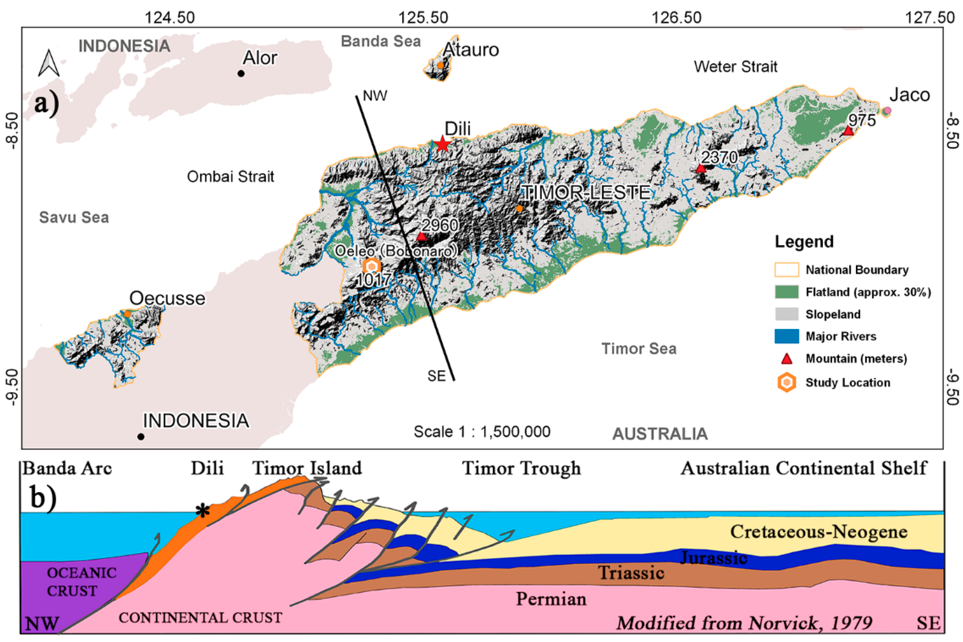
2. Location and Geoenvironmental Settings

2.1. Overview of the Country

Timor is a non-volcanic island located between the south-eastern part of the Indonesian archipelago and the northern part of the Australian continent [55]. It is approximately 500 km long and 100 km at its greatest width, elongated in the SW-NE orientation. Timor-Leste consists of the eastern half of the Timor Island, including the enclave of Oecusse in West Timor, and two islands, Ataúro and Jaco, which correspond to about 15,000 km² of territorial extension. Timor-Leste is a topographically mountainous country (Figure 1a). The flat area, with slopes in the range of 0% to 3%, occupies approximately 30% of the total country’s extension. The rest is mountainous, with slopes of between 3% and 25%. The mountain range located in the central region of the island, reaching the highest elevation at Ramelau Peak at 2960 m, belongs to the territory of Timor-Leste. This mountain range extends to the east following Matebean Peak at 2373 m and ending at Paichau Peak at 975 m. To the north side, the mountain slopes decrease, falling moderately and then almost abruptly into the ocean, characterized by a steep slope that extends practically along the entire coast. In contrast, to the south the relief is much smoother, forming a long flat coastal strip. This central region is crossed by a dense hydrographic network dividing the rainfall-runoff to the north and south through the deep and narrow valleys with short steep courses to the sea. The dominant vegetation comprises grass and shrubs, and dense forests are spatially distributed in small areas. Bouma and Kobryn [56] identified a significant level of deforestation and devegetation from 1989 to 1999. The types of soils identified in Timor-Leste are predominantly cambisols, vertisols, and fluvisols [57]. Cambisols are spatially distributed in highlands, vertisols in lowlands, and fluvisols in coastal zones. Currently, the soil erosion levels are considered catastrophic [3,56,57,58]. The rain distribution is affected by the mountainous terrain and the position of the island of Timor relative to the Australian mainland and the Indonesian archipelago (Figure 1a). The annual seasons are determined by the Australian monsoon (SE) and the Asian monsoon (NW). The geography generates two distinct rainfall patterns: 1) the Northern Monomodal Rainfall Pattern, where the rainy season starts in December, has a duration of 4 to 6 months, and affects most parts of the north of the country and some eastern regions; 2) the Southern Bimodal Rainfall Pattern, where the rainy season starts in December and has a duration of 7 to 9 months, with two rainfall peaks starting in December and May, affecting the southern side of the country [57,59,60,61,62]. The rainfall is extremely intense, with an annual average of more than 1500 mm in the mountainous areas and less than 1500 mm in the lowland areas [57,59,60,61]. Timor is an island of rapid and relatively recent formation, located at the collisional margin between the oceanic Banda volcanic arc and the Australian continental margin. This location is characterized by deformation, uplift movement, and high seismic activity (Figure 1a). Several theories about the tectonic evolution of Timor have been proposed related to its structural complexity (Figure 1b). Two main tectonic models have been discussed—the overthrust model [55,63,64] and the imbricate model [65,66,67]. This tectonic mechanism is reflected in the mountainous characteristics of the island, followed by the fragmented and chaotic structures of thrust and fold zones illustrated by Norvick [68] in Figure 1b. Measurements indicate that the Australian continent is moving ~7 cm/yr NNE relative to the South Banda arc [69]. Geologically, Timor Island presents a great diversity and complexity in its lithology and is characterized typically by soft sediments, shale, sand, and limestone [55].

2.2. Bobonaro Region

The Bobonaro region is located in the center of Timor Island; covers 216 km²; and is located 180 km from the capital, Dili. Its geographic coordinates range between 125.21694183° and −9.13041210°: 125.43438720° and −8.95447254°, and it is approximately 1000 m above the mean sea level (Figure 1a). The Bobonaro Administrative Post is subdivided into 18 villages, with a total population of 24,719 [70]. This area is part of the Bobonaro Scaly Clay Formation, previously defined by Audley-Charles [55], with a type-locality beside the Lomea River, east of Bobonaro City. Bobonaro Scaly Clay, also well known as Bobonaro mélange or broken formation, is much more widespread throughout Timor-Leste than any other existing geological formation. Bobonaro Scaly Clay is a lithotectonic unit composed mostly of broken, clay-rich layers that are mixed to varying degrees with structurally and stratigraphically overlying units. The layers range in thickness from thin to over 2000 m and contain blocks of all of the stratigraphic units in Timor, as well as serpentinites and metaigneous rocks, surrounded by a clay matrix [71]. The matrix clay of the Bobonaro mélange is mostly composed of bentonitic clay with 35% average smectite [72]. This type of clay commonly produces discontinuities and shear planes that lead to unstable hill slopes [73]. The erosion of the Bobonaro Scaly clay formation due to the tropical conditions gives rugged topography to the region characterized by deep gullies, landslides, and knobbly hillsides [55].

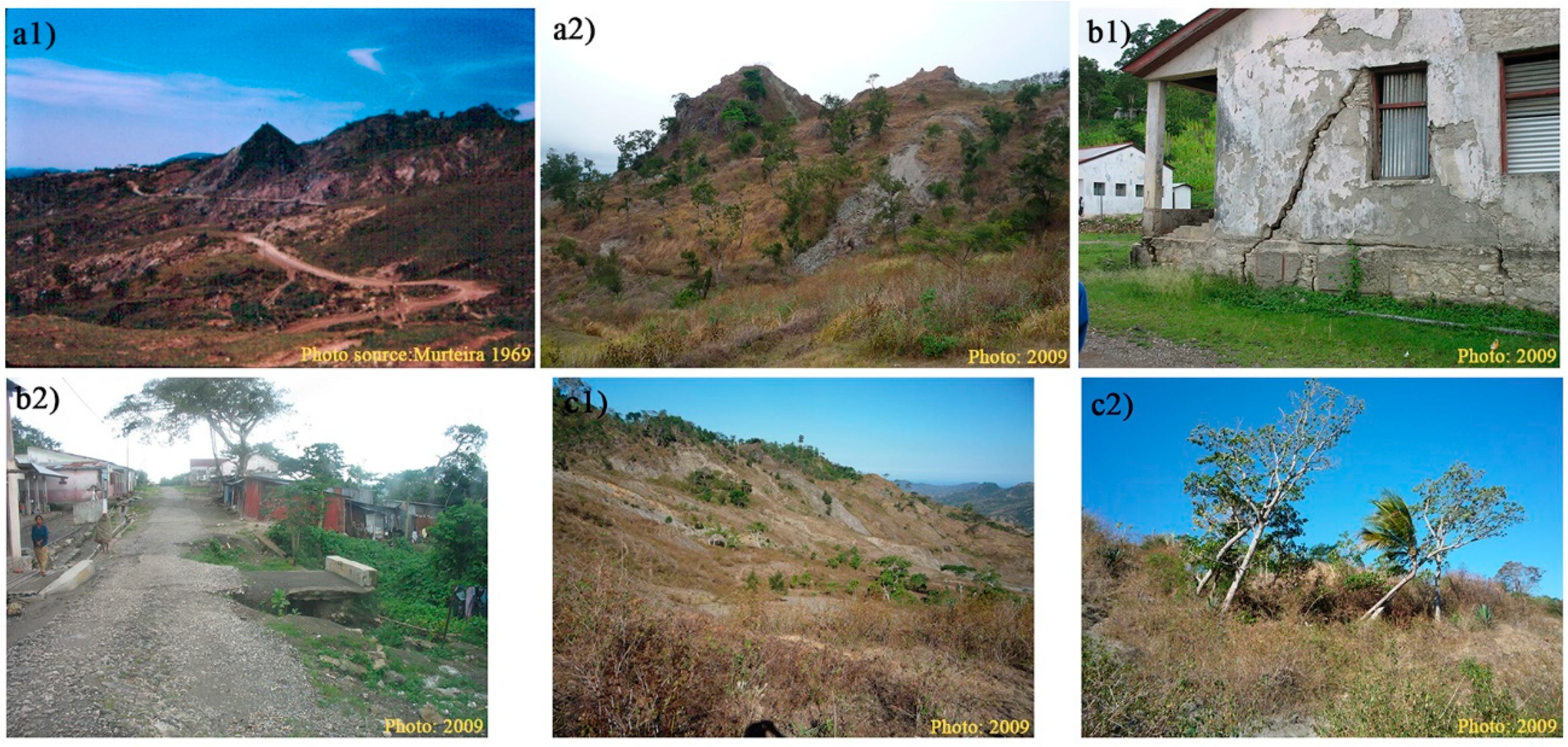
2.3. Historical Ground Deformation

A large number of ground deformations, exposed by a variety of mechanisms and magnitudes, are spatially well distributed in the Bobonaro region. It has been possible to collect valuable information related to this phenomenon from the local people, extending from the past years to the present (Figure 2). The biggest landslide was registered in Fatuk Monu (literally Rock Fall) at the end of the 18th century. The phenomenon took place at the end of the wet season. There was no rain at the time; however, all the springs in the area were over-watered, which was not usual. At the time, Fatuk Monu was very populated with the Lamak Hitu ethnic people. This landslide occurrence was clearly remembered and passed down by people in the local culture by means of legends, prayers, dances, etc., and is reflected in toponymy and in the names given to the new settlements or villages established in the Bobonaro region. The landslide completely destroyed the populated area, causing material damage as well as the loss of many human lives. After the catastrophe, new settlement sites were established in the south—now Malilait, the current capital of the Bobonaro Administrative Post—and in the northern villages of Taimea and Grotu. In 1918, at the same place the Portuguese administration built a road passing through the old landslide area, linking Malilait and Taimea. However, since 1969 the road has been impassable. At present, there are no traces of the road. The slope movement in that area has remained active on a small scale. In January 1983, a large ground movement occurred in the center of Bobonaro City, affecting the public buildings constructed in early 1956 as well as people, houses, and the main road, causing material damage but without the loss of human lives. Cracks on the walls and floors of buildings and on public roads have increased over time, caused by the phenomena of slow movement and slopes. In February 2003, in the village of Aiassa a landslide occurred after rain continuously fell for more than four hours. The landslide started at midnight and continued until early morning, destroying one house and 40 parcels of garden land but without the loss of any human lives.

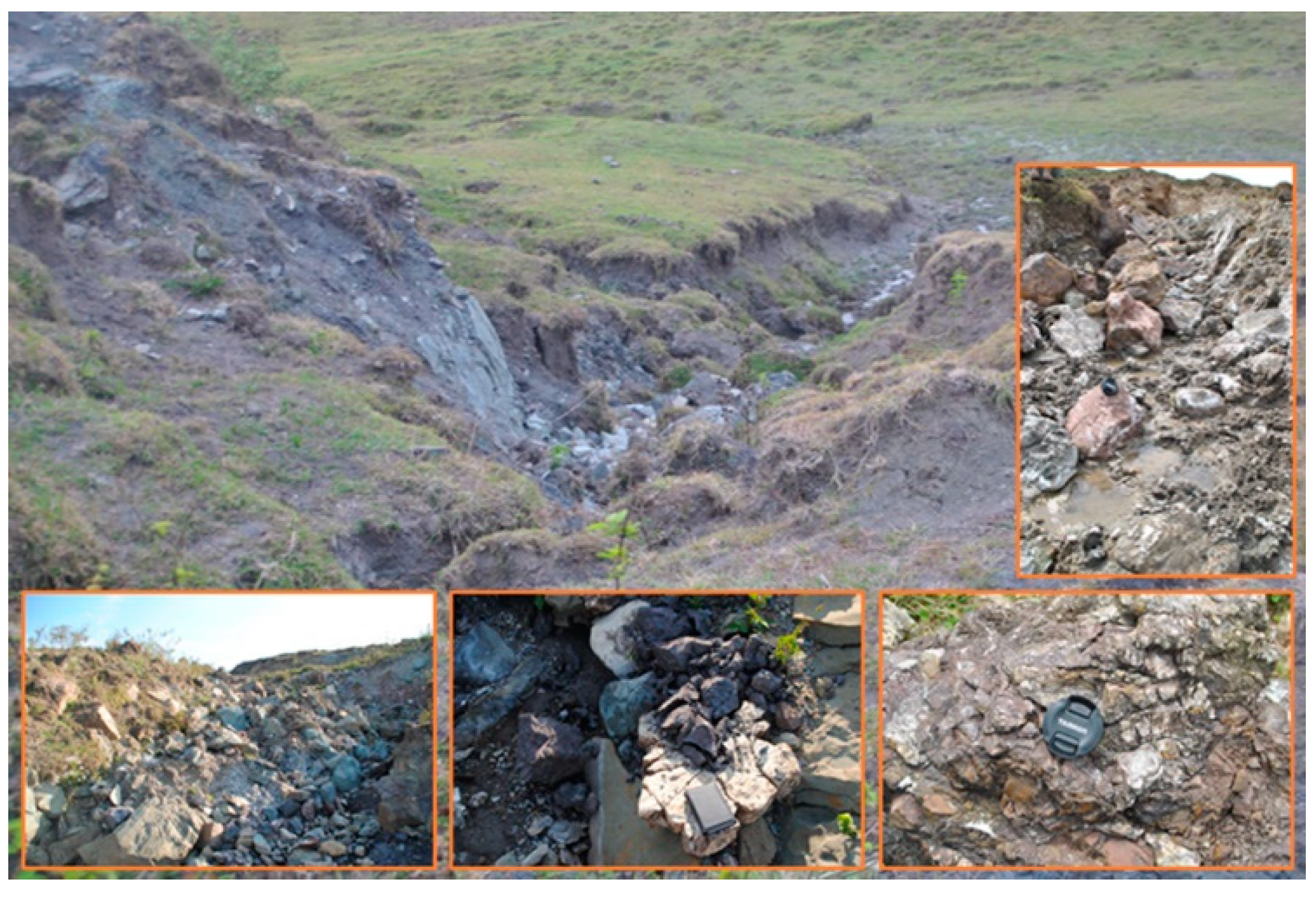
2.4. Types of Mechanism

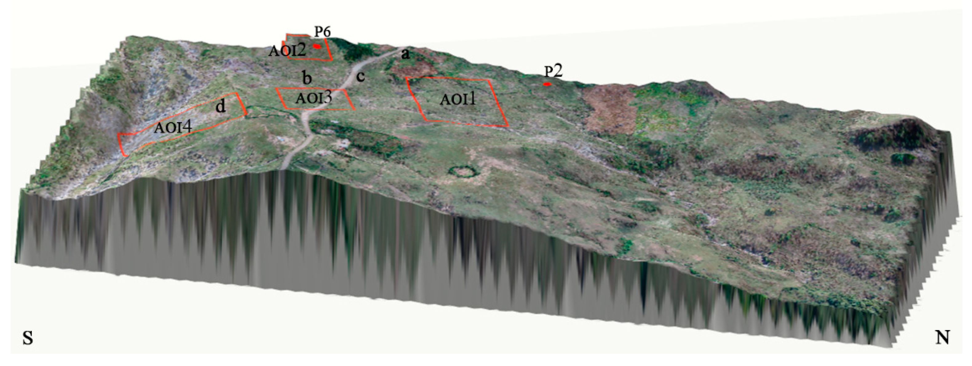
The processes of ground deformation and landslides observed in the Bobonaro region are herein described following the Varnes [74] classifications. The types of mechanism vary from simple and isolated occurrences to more complex ones in a chain sequence from the peak of the mountain to the base. Figure 3 illustrates the types of mechanism and their locations classified into three groups: (i) slopes closest to the top of the mountain; (ii) steep slopes or ravines; and (iii) more at the base of the slopes—that is, specifically in the areas near watercourses.

Alongside the riverbank, the slope became unstable and consequently it collapsed and was followed by other types of slope movements such as fall, topple, spread, sliding, and flow. It also resulted in the appearance of the deposition of detritus material close to the watercourses as a result of the flow-type movement. Normally, sliding movements (translational or rotational) and debris flows contain large amounts of materials that can intercept the main streamline, consequently generating a natural dam with the capacity to temporarily flood a wide area until the sediment is removed and transported naturally by the water stream.

2.5. Study Area

The study area is located in a highland, about 1000 m in altitude, within an area of 0.35 km² of extension. Its surface is covered by grassland vegetation, with a moderate natural slope of around 12°. The natural condition of the study area is presented in a 3D model image along with the locations of the Points of Interest (POI) and Areas of Interest (AOI) (Figure 4). The material outcrops consist of essentially serpentinites and metaigneous rocks and are surrounded by a clay matrix (Figure 5). In 2007, a few months after the construction of the road the section near the village of Oeleo began deforming. This phenomenon has continued to the present, causing damage to residential housing, agriculture fields, roads, and other infrastructure. Every year, this section of the road is affected by ground deformation, often making it impassable to vehicles during the rainy season. The area around this road section has widely shown ground surface deformation features. Recent evidence of the ground surface deformation includes degraded road conditions, a high density of ground fissures and cracks, slope movements, new water ponds, tilted electrical poles, and the ruins of a masonry house, which are marked in Figure 4 and Figure 6. Additional relevant information was collected from the local people and Google Earth historical imagery in order to confirm the evidence. The present authors clarified and recorded the four most notable pieces of evidence. The first three occurred at AOI2 and AOI3 and the fourth at AOI4. First, a masonry house was destroyed by a landslide in January 2017 during heavy rain, with material losses but no victims. Second, the electrical transmission line established in 2012 was deviated from the original alignment and tilted. Third, very frequent road restoration work has been performed during the rainy season with minimum conditions to allow the passage of transport vehicles. Fourth, a small slope failure induced by an earthquake event on 24 June 2019, with a 7.3 magnitude, occurred 518 km from the epicenter with a focal depth of 212 km.

3. Data

In this paper, deformation measurements from Advanced Land Observation Satellite (ALOS) Phased Array type L-band Synthetic Aperture Radar (PALSAR) are presented. The first ALOS1 PALSAR1 was in operation from 2006–2011, and the second ALOS2 PALSAR2 has been in operation from 2015 to the present day. These SAR datasets were provided by the Japan Aerospace Exploration Agency (JAXA). The first dataset, composed of 22 SAR images collected from PALSAR1, covered the period from 22 January 2007 to 2 February 2011. The second dataset, composed of 13 SAR images collected from PALSAR2, covered the period from 10 February 2015 to 2 April 2019. High-resolution orthomosaic and DEM images were collected on 19 August 2017 by employing Small UAV Photogrammetry DJI Mavic Pro. The earthquake data downloaded from the United States Geological Survey (USGS) Earthquake Catalogue covered the two periods of study. Timor-Leste rainfall data has not been well recorded since 1974. To overcome this unavailability of rainfall data, it was necessary to use the data published by the Climate Forecast System Reanalysis (CFSR) of the National Centers for Environmental Prediction (NCEP). Fortunately, the first study period—January 2007 to February 2011—covered daily rainfall data, with a spatial resolution of 38 km. Two imaginary stations—namely, p-891253 and p-921250—located above the mountainous area were selected. For the second period, a HOBO ground station rainfall data logger with a resolution of 0.2 mm per tip was installed 2 km from the study area. The data collection was conducted from 7 March 2007 until 2 April 2019, partially covering the second period.

4. Methodology and Processes

4.1. SBAS DInSAR

Synthetic Aperture Radar (SAR) is a specific imaging radar system mounted on an aircraft or artificial satellite [75]. SAR provides high-resolution remote sensing images, independent of daytime (day/night) and weather. The images acquired from SAR are used for vast applications and research in fields such as geoscience, environmental, climate change, and Earth system observation [76]. Interferometric SAR (InSAR) is a technique for deriving the topographic surface or digital elevation model (DEM) by extracting the signal phase changes (interference) from two SAR images acquired from the same position in repeated orbits of the satellite.

Differential interferometry SAR (DInSAR) is a technique for measuring the deformation of the Earth’s surface induced by natural and or artificial processes. In DInSAR, the topographic contribution is removed by using out-source elevation information from a DEM. However, during the interferogram processing by the DInSAR technique, besides the deformation component some residual terms appear due to the topographic pattern and defects in the orbital parameters [77]. To enhance the accuracy of DInSAR, some methods have been proposed based on persistent scatters (PS) and distributed scatters (DS). The two most widely used methods are called Permanent Scatters InSAR (PSI) [29] and Small Baseline Subsets (SBAS) DInSAR [27].

4.2. SBAS DInSAR Processing

For the time-series analysis, this study employs the SBAS method that was proposed by Berardino [27]. The SBAS method was applied for both datasets—PALSAR1 and PALSAR2—separately for the first period and the second period. The HH polarization data were selected to generate the interferograms. The topography phase component was removed using the SRTM1 DEM data with a 30 m resolution which was acquired in 2000. The perpendicular and temporal threshold criteria for SBAS processing depend on the conditions of the study area [78]. A perpendicular baseline up to 5 km can be used for ALOS PALSAR data, since longer wavelengths are less sensitive to geometric distortion [79].

For the PALSAR1 data, the maximum perpendicular and temporal baselines of the interferogram for SBAS processing are ±2000 m and 270 days, respectively. Accordingly, 55 pairs of interferograms met the criteria. For the PALSAR2 data, the maximum perpendicular and temporal baselines of the interferogram for the SBAS processing are ±400 m and 365 days, respectively. Thus, 33 pairs of interferograms met the criteria for further processing. Figure 7a,b shows the baseline table of SBAS DInSAR for PALSAR1 and PALSAR2, respectively.

The generation of interferograms is affected by many types of noise—namely, speckle noise, orbital errors, and atmospheric errors. In order to reduce the noise, an interferogram multi-looks operation was conducted. The number of range looks was 2 and the number of azimuth looks was 4 for PALSAR1, while the number of range looks was 1 and the number of azimuth looks was 3 for PALSAR2. Interferogram multi-looking is effective for reducing noise with the trade-off of a worse spatial resolution [75]. In addition, to improve the quality of the interferograms, the Goldstein filter [80] was applied. The unwrapping process was then conducted for each interferogram by using the robust minimum cost flow (MCF) algorithm [81]. In the unwrapping step, the coherence threshold was set at 0.2 both for PALSAR1 and PALSAR2, which means that the pixels with a coherence of less than 0.2 were removed and not involved in the calculation.

The orbital error fringes interfered in some interferograms [75]. To redefine these orbital fringe errors, a 2nd order polynomial estimation in the azimuth and range directions was applied and calibrated with the number of ground control points (GCPs). A total of 134 GCPs located in Maliana and Zumalae were used for PALSAR1, and 36 GCPs located in Maliana were used for PALASR2 (Figure 8b). The GCPs are located on flat land where the unwrapped phase error is minimum. A repeated unwrapping process will redefine the interferograms. The atmospheric phase screen (APS) is the dominant error source for InSAR [82]. A custom spatio-temporal filter—whose spatial low pass window size is 1.2 km × 1.2 km and whose temporal high pass size is 365 days—was applied to reduce those errors. After minimizing all the associated errors, the next step was the geocoding process and image resampling. For this process, the temporal coherence threshold coefficient was defined at 0.4 for PALSAR1 and 0.2 for PALSAR2. Finally, the maps for the time-series LOS displacement were generated by each dataset. The spatial resolution was 15 m × 15 m for PALSAR1 and 10 m × 10 m for PALSAR2. An example of an interferogram map, coherence map, and LOS mean displacement velocity map for both PALSAR1 and PALSAR2 are presented in Appendix A.

4.3. UAV Photogrammetry

UAV photogrammetry is a small remote sensing platform for acquiring high-resolution images of the ground surface. High-resolution and georeferenced UAV photogrammetry images allow for a wider range of applications with much greater detail and accuracy than satellite data. The Structure-from-Motion (SfM) technique is capable of generating a georeferenced high-resolution orthomosaic and DEM [42,43,44,45,49,50,51,54,83]. The UAV DEM has a high accuracy in the centimeter to millimeter order for estimating and measuring ground surface deformation. Henceforward, in the Geographic Information System (GIS) environment, other information can be generated from the DEM, such as contour lines, the cross section and profile, hillshade, slope, aspect, and water flow.

A small UAV, DJI Mavic Pro, was employed for ground mapping in the study area. The DJI Mavic Pro has been used in various fields of research [49,50,83,84,85,86,87,88,89,90]. This is a foldable drone with a flight weight of 743 g, a maximum flight time of about 27 min, and a maximum flight distance of 13 km under a no-wind condition. The platform is equipped with one GPS/GLONASS module, the latest Inertial Measurements Unit (IMU) module and flight control stabilization technology in order to fly smoothly, and a 4K stabilized integrated gimbal and autopilot module for navigation. The camera specification is a non-metric camera with a sensor size of 1/2.3” (CMOS). It has 12.35 million pixels; a lens with a viewing angle of 78.8°, 26 mm (35 mm equivalent); an f/2.2 distortion of <1.5%; and a focus of 0.5 m to infinity. It can take images with a maximum still image size of 4000 × 3000 and is capable of direct image georeferencing. The main disadvantage of this drone is certainly its high sensitivity to wind turbulence due to its small size and light weight.

4.4. UAV Photogrammetry Data Acquisition and Processing

Drone Deploy provides a user-friendly and free application for flight planning and mapping. This application can be installed both in smart mobile devices (iOS or Android) and online access in desktop computers. It is very convenient and makes it easy to prepare all the plans and record them in the office, either hours or days before going to do the fieldwork. The online software automatically generates the flight path and is user configurable. Some adjustments are needed, such as the flight altitude, flight direction, flight mapping speeds, front and side overlap percentages, and manual camera settings, if necessary. During the flight plan configuration, the software automatically calculates the flight duration in minutes, the total area covered in hectares, the number of images, the amount of battery consumption, and the image resolution in cm/px. Once the flight plan is completed, the smart device only needs to be connected to the Internet and the Drone Deploy application opened in order to update the latest information or project. At the desired location, the smart device can be connected via USB to the drone, the proper project chosen, the preflight checklist started, and the flight initiated. The drone will automatically start the rotors, record the home point, and take off, following all the flight plan instructions and recording images in the onboard micro memory card. After completing all the instructions, the drone will fly back to land at the home point. For this study, the percentage of overlap was set to 75% for the front overlap, 65% for the side overlap, 80 m for the flight altitude, and 2.4 cm for the resolution; the camera was set to automatic mode. The survey mapping was conducted without ground control points [83,87,91,92,93].

The images collected were georeferenced in the WGS84 geographic coordinate system, including the ellipsoid altitude. The georeferenced images allow the photogrammetry software to detect the three-dimensional positions at which the images were taken. The recent improvement in the georeferenced image processing by a powerful computer and the application of computer vision modelling using the SfM technique allow the building of a three-dimensional terrain model with a high quality and low time consumption [42,49,50,83,91,94]. In this study, the SfM-based software, AgiSoft PhotoScan version 1.4.5, was employed. The output can be immediately manipulated using GIS software such as ArcGIS 10.4 and QGIS 3.4 to correct geometric errors and to extract other spatial information.

5. Results

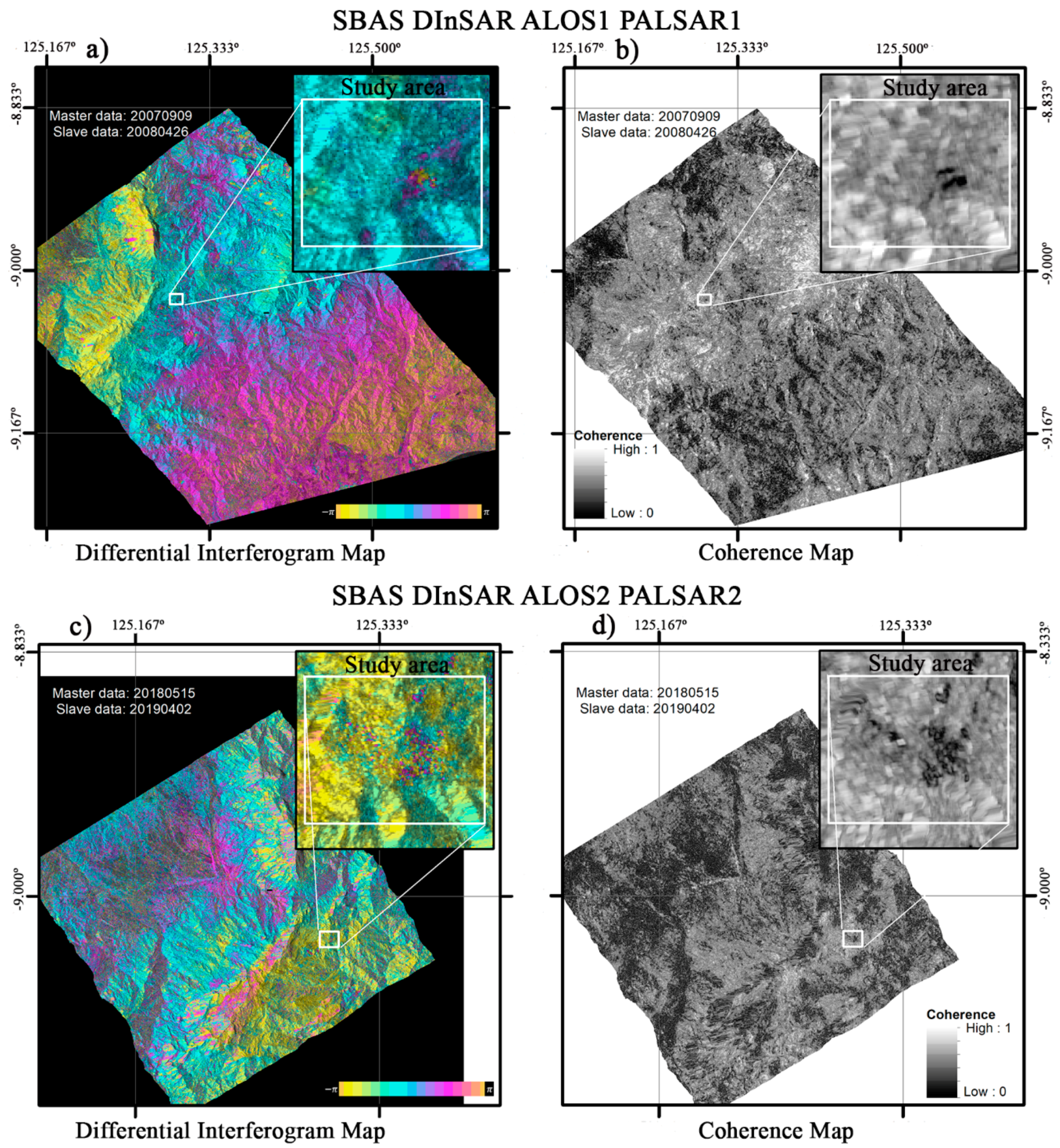
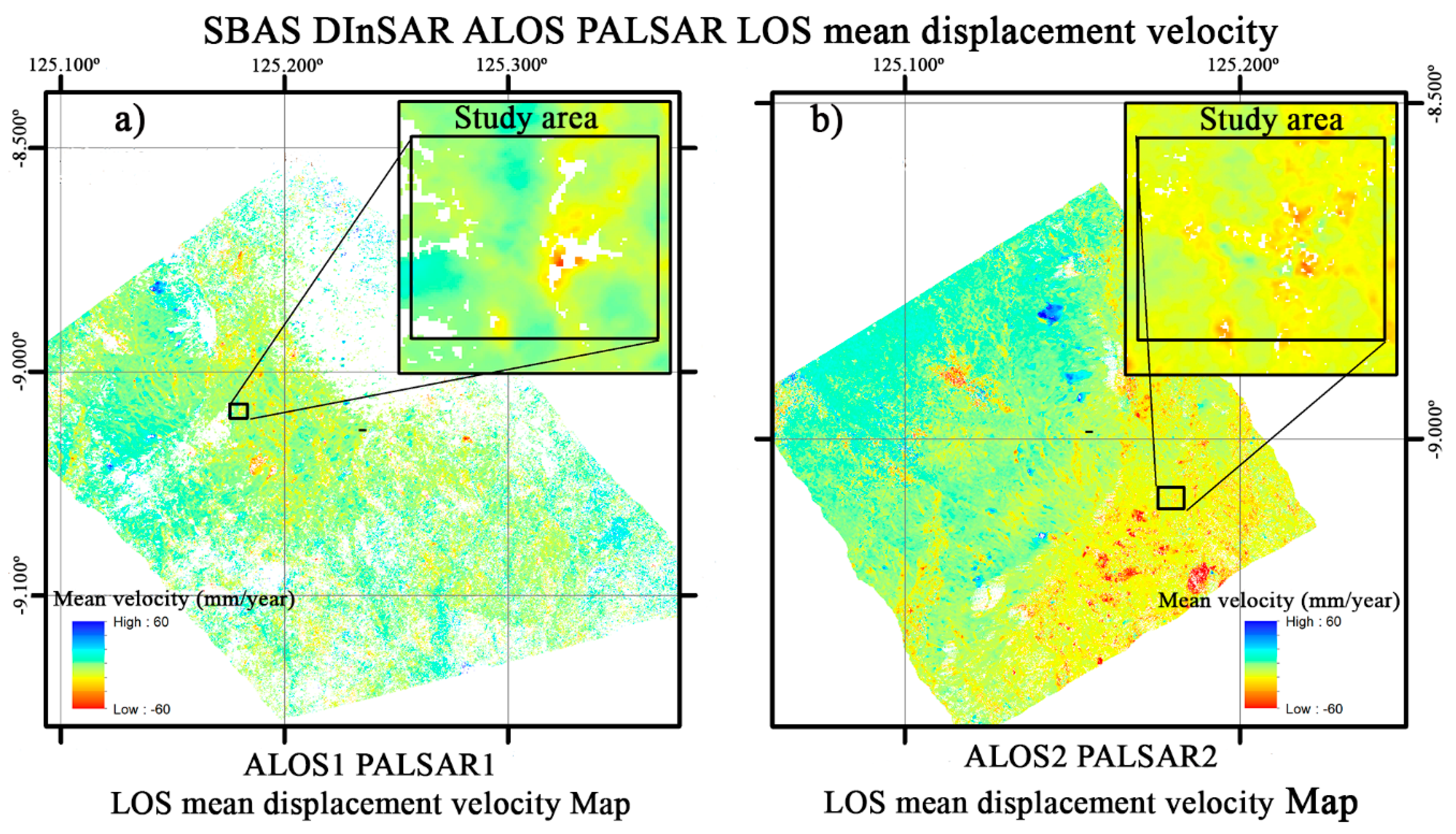
5.1. Time-Series SBAS DInSAR

The ground deformation detected by SBAS DInSAR from both PALSAR1 and PALSAR2 is presented in line of sight (LOS) displacement values and their spatial distribution (Figure 8c,d). These LOS displacement values were furthermore used for geoprocessing in GIS software environments. Seven points of interest (POIs)—namely, P1, P2, P3, P4, P5, P6, and P7—were defined around the study area near the village of Oeleo (Figure 8c,d). In order to identify the distribution of ground deformation with more detail, four areas of interest (AOIs)—AOI1, AOI2, AOI3, and AOI4—were defined (Figure 8c,d). These AOIs were applied for the first period. Six more POIs—namely, P8, P9, P10, P11, P12, and P13—were defined for the second period (Figure 8d). The definitions of the additional POIs and AOIs were based on the LOS displacement images, the recent field observations, and UAV orthomosaic image interpretation. The LOS displacement values were extracted and converted to points for further analysis. The PALSAR1 and PALSAR2 LOS displacement time-series related to P1, P2, P3, P4, P5, P6, and P7 are presented in Figure 8e,f respectively.

The PALSAR1 LOS displacement time-series values related to AOI1, AOI2, AOI3, and AOI4 were extracted and applied to calculate the mean, minimum, and maximum values. These values were used to show the ground deformation trend in Figure 9a–d, respectively. AOI2 and AOI3 show high displacement values, while AOI4 seems more stable.

The PALSAR2 LOS displacement time-series values related to P8, P9, P10, P11, P12, and P13 were extracted and are presented in Figure 9e. Based on the LOS displacement values, both POIs—P3 and P7—seemed more constant than the others during the first period. However, during the second period, P3 and P7 presented displacements as well. POIs P2 and P6 presented very high values of LOS displacement during the two periods (Figure 8e,f). In Figure 9e, P8 and P9 showed LOS displacement values of more than 200 mm compared to other POIs.

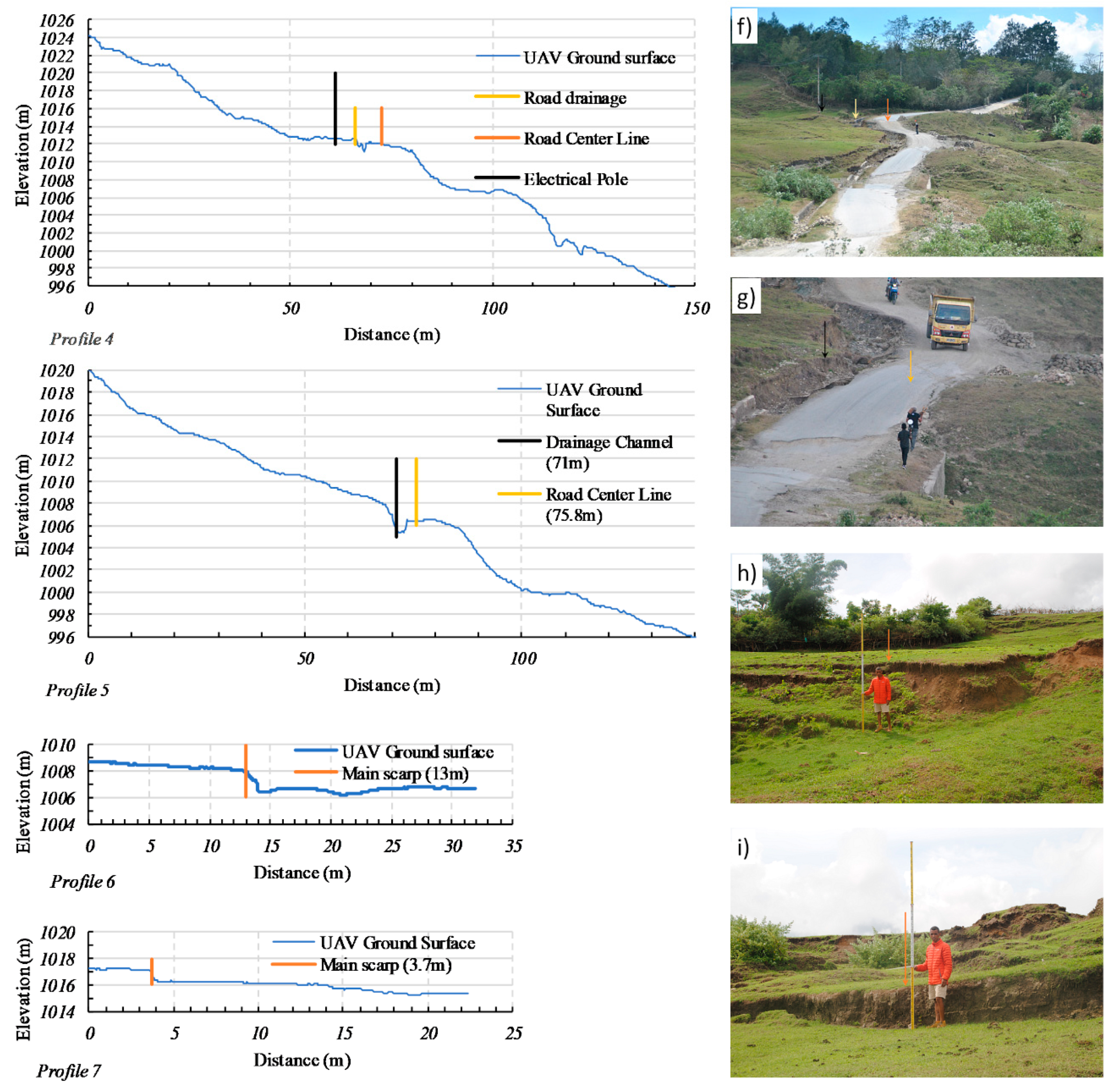
5.2. UAV Georeferenced Photogrammetry

For this study, a UAV aerial mapping mission was conducted on 19 August 2017 without the application of GCPs. The positioning system was based on a single built-in unit GPS/GLONASS module installed inside the drone. Thus, a minimum of 12 numbers from the satellite had to be achieved to get a strong signal from the GPS before starting the flight for survey mapping. This requirement is very important for obtaining good quality georeferencing images. For most of the acquired images, the quality was good, with values of quality estimation coefficients greater than 0.8, as analyzed by the Agisoft PhotoScan 1.4.5 software. It was necessary to check the image quality before proceeding to the image processing stage. For the next step, the workflow presented in the Agisoft PhotoScan software was followed. The result presented very high-resolution orthomosaic images and digital elevation models for both (Figure 10b,c). Figure 10a shows the acceptable georeferencing quality of the orthomosaic image, which matched the Google Maps Hybrid. From the orthomosaic image, it was possible to interpret and measure the ground fissures in the GIS environment with a centimeter-order accuracy. The digital elevation model allows for other spatial information, such as contour lines and surface profiles, to be generated.

6. Discussion

The ground surface deformation detected by the SBAS DInSAR derived from PALSAR1 and PALSAR2 will be discussed in this section. Multi-temporal SBAS DInSAR is a very effective technique for detecting the subsidence over a vast area. However, for detecting local ground displacement this technique still has limitations—namely, it is used in densely vegetated areas and under steep slope conditions [40]. Thus, although discussions on the precise measurements of local ground displacements are very important, they will be considered as a topic to address in future work. The advantage of this technique was taken to find the relation between the LOS displacement results and the behavior of the ground surface deformation from the past until the present. UAV georeferenced photogrammetry will be used to interpret the ground surface deformation and to confirm the latest LOS displacements synchronously.

The LOS displacement time-series clearly shows a trend in the ground deformation during these two periods of study (Figure 8e,f). The tendency was to move in the negative direction, and the LOS displacement values varied among the POIs. From Figure 8d, it is seem that the POIs have been classified into three groups—namely, Group 1 (P3 and P7), Group 2 (P1, P4 and P5), and Group 3 (P2 and P6). Group 1 was more stable during the first period. However, during the second period the LOS displacements were increasing or moving down, starting from 9 February 2016 until the end of the period. Group 2 presented uniform displacements during the first period and continued until March 2016. After that, the LOS displacements increased drastically. Group 3 presented the highest values of the LOS displacements during the first period. During the second period, the POIs in this group differed from the LOS displacement values. P6 tended to be stabilized, while P2 showed a continuous increase in the LOS displacement values during the second period. The differences in behavior between P2 and P6 reveal important information for understanding and describing the relative movement and direction of the ground deformation in this location. For this purpose, the latest PALSAR2 LOS displacements were overlayered on the UAV DEM. The results showed a good coherence between the LOS displacements and the ground surface conditions (Figure 11). As can be observed in Figure 9e, something interesting occurred in relation to the additional POIs. P8 and P9 reached LOS displacement values of above 200 mm. Further investigation will focus on the area of interest 3 (AOI3).

The next step will focus on the ground surface interpretation, based on the very high-resolution of the UAV orthomosaic and DEM (Figure 4 and Figure 12). P6 is located at the highest location at an elevation of 1030 m, and P2 is located at a lower location at an elevation of 990 m. AOI2 and AOI3 are located near P6 and AOI1 is located near P2. Based on the landslide morphology presented by Varnes [74], it was possible to identify the typical features of the ground movement or landslide. In Figure 12, some important ground morphology features—such as the main fracture, transverse fracture, internal fracture, pond water, and watercourses—can be identified. AOI2 and AOI3 are situated in the depletion zone and are characterized by crowns, main scarps, heads, and flanks. Two main scarps, several heads, and discreet flanks were identified. AOI1 lies in the accumulation zone, which is characterized by radial cracks, transverse cracks, toe ridges, and transverse ridges. Based on this ground morphology, it was assumed that the ground surface deformation occurred during the first period and that the process continued until the end of the second period. The ground is seen to be moving down, following the natural streamline in the NE direction. The ground at AOI4 is seen to be moving in the opposite direction. The slope is steeper and characterized by translational movement, and no water pond was found.

The very high-resolution orthomosaic images and DEM allowed for a more detailed interpretation of the morphology of the ground surface deformation [39]. Specific terrain profile sections were extracted from the UAV DEM (Figure 13a). For each profile section, the ground surface as well as the remarkable ground features and objects are presented in the graphs (Figure 13 and Figure 14). The results show that the ground surface deformation measurements vary from centimeters to meters in both the vertical and horizontal directions. From Profile 1, the results of the road surface elevation extracted from UAV DEM are presented and compared with the total station measurements. The graph shows a good coherence between these two measurement methods (Figure 13c). The line of Profile 2 follows the electrical pole line. It is noted that the electrical pole moved horizontally more than 4 m from the initial position (Figure 13b,d). Profile 3 represents the natural ground surface condition and a ground crack, shown in Figure 13e. Profiles 4 and 5 represent some parts of the roads that were affected by the ground deformation (Figure 14f,g). Profiles 6 and 7 represent the main scarps that were measured and illustrated in Figure 14h,i, respectively.

Additionally, the PALSAR1 and PALSAR2 LOS displacement time-series were gathered with the earthquake data from the USGS Earthquake Catalogue and the daily rainfall data from CFSR/NCEP and local ground stations in order to find their relationship in time occurrences, as presented in Figure 15. Even with a moderate slope with approximately 12 degrees of inclination, the ground deformation continues and slides in the northeast in the same direction as the watercourses. From the LOS displacement values and the UAV orthomosaic and DEM images interpretation results, some representative POIs—such as P2, P6, P8, and P9—were chosen. At the end of the second period, P8 and P9 reached maximum values of more than 200 mm. These two POIs are located on either side of the deformed road alignment (Figure 12). The relevant earthquake attributes, the magnitude scale starting from 4.5 up to the maximum recorded values, and the hypocenter depth were selected. The rainfall data available from CFSR only covered the first period. Unfortunately, for the second period the daily rainfall data were not totally collected due to time and technical limitations. The rainfall data collected from the ground station rainfall data logger partially covered the second period, starting from 7 March 2017 and continuing until the end of the period of study. The earthquake events were extracted according to the study period and the epicenter position within a radius of 100 km from the study location. For the first and second periods, 21 and 34 earthquake events were selected, respectively. The earthquakes were generally shallow, with hypocenter depths of less than 50 km for both periods.

Some previous works have confirmed these factors that influence the dynamic process of the geological and tectonic formations of the island. Audley-Charles [55] considered the tropical rainfall as the factor responsible for the rugged topography of the Bobonaro region characterized by deep gullies, landslides, and knobby hillsides, as shown in Figure 3. Due to the location of Timor Island in the arc-collision zone [55,63,64,65,66,67,68,69], Norvick [68] illustrated the tectonic mechanism and high seismic activity reflected in the mountain characteristics, followed by the fragmented and chaotic structures of the thrust and fold zones shown in Figure 1b.

In this study, some interpretations are presented based on Figure 15. During the first year, from 1 January 2007 to 1 July 2007 eight earthquake events were recorded, one with a maximum magnitude of 5.1 and practically all occurring during rainy months, however with low amounts of rainfall. The ground deformation presented the maximum value of −38.1 mm. During the fourth year, January 2010 to January 2011, six earthquake events were recorded with an average magnitude of 4.5, and the rainfall amount was higher than that of the previous years. The ground deformation presented the maximum value of −65.7 mm. However, for the third year—January 2009 to January 2010—only two earthquakes were recorded, with magnitudes of 5.1 and 5.0 and a moderate amount of rainfall. The ground deformation presented the maximum value of −46.9 mm. During the sequences of events in the second period, the earthquake reached the maximum magnitude of 6.5 and the hypocenter depth of 20 km on 4 November 2015. In the same month, 16 earthquake events were recorded, with an average magnitude of 5.0. At this stage, no rainfall contribution could be found. However, one landslide occurrence was recorded in January 2017 during heavy rainfall. Based on this evidence, it was assumed that the rainfall in 2017 was high. From November 2015 to March 2017, the ground deformation presented the maximum value of −102. 6 mm. For the next few years, the LOS displacement values showed positive evolution linked with the rainy season and seismic activity until the end of the study period. From January 2018 to April 2019, the ground deformation presented the maximum value of −82.4 mm.

It is well known that the occurrence of an earthquake with a certain magnitude or greater triggers the reactivation of landslides. However, the influence does not always appear immediately after the earthquake. On the other hand, heavy or long rainfall events induce landslides and/or changes in the ground, and their influence can appear a relatively short time after the event under specific ground conditions. This is because the time it takes rainfall water to infiltrate into the ground depends on the degree of development of the catchment areas, the permeability of the ground, and the presence of cracks in the ground [95,96]. Considering the above characteristics, it can be denied that the timing of ground deformation, earthquake events, and periodic rainfall are clearly related to and based on the results of the LOS displacement time-series for either period. As a practical approach, Figure 15 presents important information that should be considered as complementary data for this study. In future works, a more precise approach will be needed to reach an acceptable conclusion.

7. Conclusions

The natural phenomenon of ground surface deformation in Bobonaro, near the village of Oeleo, has been taking place over the years, generating a great deal of material loss for its citizens and considerable financial loss of the state budget spent in vain on road construction and maintenance.

In this study, it was proved that multi-temporal DInSAR is capable of detecting ground surface deformation on a local scale within the extension of an area of less than 1 km². The results of the LOS displacement showed the trend in the ground surface deformation during the two periods of study. The main advantage of this technique is that it is useful for ground surface deformation screening, even in small areas of interest and under moderate slope conditions. The latest PALSAR2 LOS displacement corresponds well with the ground surface deformation morphonology mapped by the small UAV DJI Mavic Pro. UAV high-resolution data, obtained by orthomosaic means and DEM, were useful for making interpretations and performing highly accurate measurements of the ground surface deformation. The measurements varied from centimeters to meters in both the vertical and horizontal directions. Furthermore, on-site field observations were used to clarify the UAV photogrammetry results. The evidence given in this work shows that the DInSAR and UAV photogrammetry techniques, used in combination, present good results.

This combination is one of the solutions for monitoring ground surface deformation in Timor-Leste. A detailed mapping of the ground deformation will serve as a base for developing further specialized fields of study related to this phenomenon, such as geological structures, geomorphology, climate and hydrology, the geotechnical properties of the rock, and excavation engineering. The achievements of these studies will contribute to supporting the infrastructure development specifically for road design and construction and generally to the risk management strategies of the country.

The results of the LOS displacement time-series showed that the time occurrence of the ground deformation, earthquake sequences, and periodic rainfalls are notably related. From the first period, it was found that earthquakes and rainfalls sometimes took place consecutively or simultaneously. It might be possible that the ground deformation was initiated by an earthquake, even that of a moderate magnitude, and that months or years after the rainfall it certainly contributed to the continuing process of ground surface deformation.

References

1. Timor-Leste Strategic Development Plan; Democratic Republic of Timor-Leste: Dili, Timor-Leste, 2011. Available online: http://timor-leste.gov.tl/wp-content/uploads/2011/07/Timor-Leste-Strategic-Plan-2011-20301.pdf (accessed on 22 June 2017).
2. Baze Dadus Dezastres Timor-Leste; Democratic Republic of Timor-Leste: Dili, Timor-Leste, 2019. Available online: http://www.tldd.mss.gov.tl/ (accessed on 20 January 2019).
3. Barnett, J.; Dessai, S.; Jones, R.N. Vulnerability to climate variability and change in East Timor. AMBIO J. Hum. Environ. 2007, 36, 372–379. [Google Scholar] [CrossRef]
4. Cook, A.D.; Suresh, V.; Nair, T.; Foo, Y.N. Integrating disaster governance in Timor-Leste: Opportunities and challenges. Int. J. Disaster Risk Reduct. 2019, 35, 1–12. [Google Scholar] [CrossRef]
5. Corominas, J.; van Westen, C.; Frattini, P.; Cascini, L.; Malet, J.P.; Fotopoulou, S.; Catani, F.; Van Den Eeckhaut, M.; Mavrouli, O.; Agliardi, F.; et al. Recommendations for the quantitative analysis of landslide risk. Bull. Eng. Geol. Environ. 2014, 73, 209–263. [Google Scholar] [CrossRef]
6. Palenzuela, J.A.; Jiménez-Perálvarez, J.D.; El Hamdouni, R.; Alameda-Hernández, P.; Chacón, J.; Irigaray, C. Integration of LiDAR data for the assessment of activity in diachronic landslides: A case study in the Betic Cordillera (Spain). Landslides 2016, 13, 629–642. [Google Scholar] [CrossRef]
7. Kjekstad, O.; Highland, L. Economic and Social Impacts of Landslides. In Landslides-Disaster Risk Reduction; Springer: Berlin/Heidelberg, Germany, 2009; pp. 573–587. [Google Scholar] [CrossRef]
8. Ding, X.; Ren, D.; Montgomery, B.; Swindells, C. Automatic monitoring of slope deformations using geotechnical instruments. J. Surv. Eng. 2000, 126, 57–68. [Google Scholar] [CrossRef]
9. Demoulin, A.; Glade, T. Recent landslide activity in Manaihan, East Belgium. Landslides 2004, 1, 305–310. [Google Scholar] [CrossRef]
10. Duc, D.M. Rainfall-triggered large landslides on 15 December 2005 in Van Canh district, Binh Dinh province, Vietnam. Landslides 2013, 10, 219–230. [Google Scholar] [CrossRef] [Green Version]
11. Shimizu, N.; Nakashima, S.; Masunari, T. ISRM suggested method for monitoring rock displacements using the Global Positioning System (GPS), Rock Mech. Rock Eng. 2014, 47, 313–328. [Google Scholar] [CrossRef]
12. Uhlemann, S.; Smith, A.; Chambers, J.; Dixon, N.; Dijkstra, T.; Haslam, E.; Meldrum, P.; Merritt, A.; Gunn, D.; Mackay, J. Assessment of ground-based monitoring techniques applied to landslide investigations. Geomorphology 2016, 253, 438–451. [Google Scholar] [CrossRef] [Green Version]
13. Ramesh, M.V.; Vasudevan, N. The deployment of deep-earth sensor probes for landslide detection. Landslides 2012, 9, 457–474. [Google Scholar] [CrossRef]
14. Chang, D.T.T.; Tsai, Y.S.; Yang, K.C. Study of real-time slope stability monitoring system using wireless sensor network. Telkomnika 2013, 11, 1478–1488. [Google Scholar]
15. Walstram, J.; Chandler, J.H.; Dixon, N.; Dijkstra, T.A. Aerial photography and digital photogrammetry for landslide monitoring. Geol. Soc. Lond. Spec. Publ. 2007, 283, 53–63. [Google Scholar] [CrossRef]
16. Jaboyedoff, M.; Oppikofer, T.; Abellán, A.; Derron, M.H.; Loye, A.; Metzger, R.; Pedrazzini, A. Use of LIDAR in landslide investigations: A review. Nat. Hazards 2012, 61, 5–28. [Google Scholar] [CrossRef] [Green Version]
17. González-Díez, A.; Fernández-Maroto, G.; Doughty, M.W.; De Terán, J.D.; Bruschi, V.; Cardenal, J.; Pérez, J.L.; Mata, E.; Delgado, J. Development of a methodological approach for the accurate measurement of slope changes due to landslides, using digital photogrammetry. Landslides 2014, 11, 615–628. [Google Scholar] [CrossRef]
18. Ciampalini, A.; Raspini, F.; Frodella, W.; Bardi, F.; Bianchini, S.; Moretti, S. The effectiveness of high-resolution LiDAR data combined with PSInSAR data in landslide study. Landslides 2016, 13, 399–410. [Google Scholar] [CrossRef] [Green Version]
19. Gorsevski, P.V.; Brown, M.K.; Panter, K.; Onasch, C.M.; Simic, A.; Snyder, J. Landslide detection and susceptibility mapping using LiDAR and an artificial neural network approach: A case study in the Cuyahoga Valley National Park, Ohio. Landslides 2016, 13, 467–484. [Google Scholar] [CrossRef]
20. Cigna, F.; Banks, V.J.; Donald, A.W.; Donohue, S.; Graham, C.; Hughes, D.; McKinley, J.M.; Parker, K. Mapping ground instability in areas of geotechnical infrastructure using satellite InSAR and Small UAV surveying: A case study in Northern Ireland. Geosciences 2017, 7, 51. [Google Scholar] [CrossRef] [Green Version]
21. Singhroy, V. SAR integrated techniques for geohazard assessment. Adv. Space Res. 1995, 15, 67–78. [Google Scholar] [CrossRef]
22. Comer, D.C.; Chapman, B.D.; Comer, J.A. Detecting landscape disturbance at the Nasca lines using SAR data collected from airborne and satellite platforms. Geosciences 2017, 7, 106. [Google Scholar] [CrossRef] [Green Version]
23. Farahmand, A.; AghaKouchak, A. A satellite-based global landslide model. Nat. Hazards Earth Syst. Sci. 2013, 13, 1259–1267. [Google Scholar] [CrossRef]
24. Hong, Y.; Adler, R.E.; Huffman, G.J. Satellite remote sensing for global landslide monitoring. Eos Trans. AGU 2007, 88, 357–358. [Google Scholar] [CrossRef] [Green Version]
25. Sassa, K.; Nagai, O.; Solidum, R.; Yamazaki, Y.; Ohta, H. An integrated model simulating the initiation and motion of earthquake and rain induced rapid landslides and its application to the 2006 Leyte landslide. Landslides 2010, 7, 219–236. [Google Scholar] [CrossRef]
26. Massonnet, D.; Feigl, K.L. Radar interferometry and its application to changes in the Earth’s surface. Rev. Geophys. 1998, 36, 441–500. [Google Scholar] [CrossRef] [Green Version]
27. Berardino, P.; Fornaro, G.; Lanari, R.; Sansosti, E. A new algorithm for surface deformation monitoring based on small baseline differential SAR interferograms. IEEE Trans. Geosci. Remote Sens. 2002, 40, 2375–2383. [Google Scholar] [CrossRef] [Green Version]
28. Necsoiu, M.; Hooper, D.M. Use of Emerging InSAR and LiDAR Remote Sensing Technologies to Anticipate and Monitor Critical Natural Hazards; Volume 58: Building Safer Communities—Risk Governance, Spatial Planning and Responses to Natural Hazards; NATO Science for Peace and Security, Series E: Human and Societal Dynamics; Paleo, U.F., Ed.; IOS Press: Amsterdam, The Netherlands, 2009; pp. 246–267. [Google Scholar] [CrossRef]
29. Ferretti, A.; Prati, C.; Rocca, F. Permanent scatterers in SAR interferometry. IEEE Trans. Geosci. Remote Sens. 2001, 39, 8–20. [Google Scholar] [CrossRef]
30. Raucoules, D.; Colesanti, C.; Carnec, C. Use of SAR interferometry for detecting and assessing ground subsidence. Comptes Rendus Geosci. 2007, 339, 289–302. [Google Scholar] [CrossRef]
31. Guzzetti, F.; Manunta, M.; Ardizzone, F.; Pepe, A.; Cardinal, M.; Zeni, G.; Paola, R.; Lanari, R. Analysis of ground deformation detected using the SBAS DInSAR technique in Umbria, Central Italy. Pure Appl. Geophys. 2009, 166, 1425–1459. [Google Scholar] [CrossRef]
32. Samsonov., S.; Beavan, J.; González, P.J.; Tiampo, K.; Fernández, J. Ground deformation in the Taupo Volcanic Zone, New Zealand, observed by ALOS PALSAR interferometry. Geophys. J. Int. 2011, 187, 147–160. [Google Scholar] [CrossRef] [Green Version]
33. Ng, A.H.M.; Ge, L.; Li, X.; Abidin, H.Z.; Andreas, H.; Zhang, K. Mapping land subsidence in Jakarta, Indonesia using persistent scatterer interferometry (PSI) technique with ALOS PALSAR. Int. J. Appl. Earth Obs. Geoinf. 2012, 18, 232–242. [Google Scholar] [CrossRef]
34. García-Davalillo, J.C.; Herrera, G.; Notti, D.; Strozzi, T.; Álvarez-Fernández, I. DInSAR analysis of ALOS PALSAR images for the assessment of very slow landslides: The Tena Valley case study. Landslides 2014, 11, 225–246. [Google Scholar] [CrossRef]
35. Necsoiu, M.; McGinnis, R.N.; Hooper, D.M. New insights on the Salmon Falls Creek Canyon landslide complex based on geomorphological analysis and multitemporal satellite InSAR techniques. Landslides 2014, 11, 1141–1153. [Google Scholar] [CrossRef]
36. Jebur, M.N.; Pradhan, B.; Tehrany, M.S. Using ALOS PALSAR derived high-resolution DInSAR to detect slow-moving landslides in tropical forest: Cameron Highlands, Malaysia. Geomat. Nat. Hazards Risk 2015, 6, 741–759. [Google Scholar] [CrossRef] [Green Version]
37. Calvello, M.; Peduto, D.; Arena, L. Combined use of statistical and DInSAR data analyses to define the state of activity of slow-moving landslides. Landslides 2017, 14, 473–489. [Google Scholar] [CrossRef]
38. Morishita, Y.; Kobayashi, T.; Yarai, H. Three-dimensional deformation mapping of a dike intrusion event in Sakurajima in 2015 by exploiting the right-and left-looking ALOS-2 InSAR. Geophys. Res. Lett. 2016, 43, 4197–4204. [Google Scholar] [CrossRef] [Green Version]
39. Lu, X.; Sun, X. Ground Subsidence Monitoring in Cheng Du Plain Using DInSAR SBAS Algorithm. In International Conference on Geo-Informatics in Resource Management and Sustainable Ecosystem; Springer: Singapore, 2017; pp. 535–545. [Google Scholar] [CrossRef]
40. Yastika, P.E.; Shimizu, N.; Abidin, H.Z. Monitoring of long-term land subsidence from 2003 to 2017 in coastal area of Semarang, Indonesia by SBAS DInSAR analyses using Envisat-ASAR, ALOS-PALSAR, and Sentinel-1A SAR data. Adv. Space Res. 2019, 63, 1719–1736. [Google Scholar] [CrossRef]
41. Gong, J.; Wang, D.; Li, Y.; Zhang, L.; Yue, Y.; Zhou, J.; Song, Y. Earthquake-induced geological hazards detection under hierarchical stripping classification framework in the Beichuan area. Landslides 2010, 7, 181–189. [Google Scholar] [CrossRef]
42. Niethammer, U.; James, M.R.; Rothmund, S.; Travelletti, J.; Joswig, M. UAV-based remote sensing of the Super-Sauze landslide: Evaluation and results. Eng. Geol. 2012, 128, 2–11. [Google Scholar] [CrossRef]
43. Lucieer, A.; Jong, S.M.D.; Turner, D. Mapping landslide displacements using Structure from Motion (SfM) and image correlation of multi-temporal UAV photography. Prog. Phys. Geogr. 2014, 38, 97–116. [Google Scholar] [CrossRef]
44. Turner, D.; Lucieer, A.; de Jong, S. Time series analysis of landslide dynamics using an unmanned aerial vehicle (UAV). Remote Sens. 2015, 7, 1736–1757. [Google Scholar] [CrossRef] [Green Version]
45. Peppa, M.V.; Mills, J.P.; Moore, P.; Miller, P.E.; Chambers, J.E. Accuracy assessment of a UAV-based landslide monitoring system. ISPRS Int. Arch. Photogramm. Remote Sens. Spat. Inf. Sci. 2016, 41, 895–902. [Google Scholar] [CrossRef]
46. Peternel, T.; Kumelj, Š.; Oštir, K.; Komac, M. Monitoring the Potoška planina landslide (NW Slovenia) using UAV photogrammetry and tachymetric measurements. Landslides 2017, 14, 395–406. [Google Scholar] [CrossRef]
47. Fan, X.; Xu, Q.; Scaringi, G.; Dai, L.; Li, W.; Dong, X.; Zhu, X.; Pei, X.; Dai, K.; Havenith, H.B. Failure mechanism and kinematics of the deadly June 24th 2017 Xinmo landslide, Maoxian, Sichuan, China. Landslides 2017, 14, 2129–2146. [Google Scholar] [CrossRef]
48. Hu, S.; Qiu, H.; Pei, Y.; Cui, Y.; Xie, W.; Wang, X.; Yang, D.; Tu, X.; Zou, Q.; Cao, P.; et al. Digital terrain analysis of a landslide on the loess tableland using high-resolution topography data. Landslides 2018, 16, 617–632. [Google Scholar] [CrossRef]
49. Ma, S.; Xu, C.; Shao, X.; Ahang, P.; Liang, X.; Tian, Y. Geometric and kinematic features of a landslide in Mabian Sichuan, China, derived from UAV photography. Landslides 2018, 16, 373–381. [Google Scholar] [CrossRef]
50. O’Driscoll, J. Landscape applications of photogrammetry using unmanned aerial vehicles. J. Archaeol. Sci. Rep. 2018, 22, 32–44. [Google Scholar] [CrossRef]
51. Rossi, G.; Tanteri, L.; Tofani, V.; Vannocci, P.; Moretti, S.; Casagli, N. Multitemporal UAV surveys for landslide mapping and characterization. Landslides 2018, 15, 1045–1052. [Google Scholar] [CrossRef] [Green Version]
52. Zhu, L.; Deng, Y.; He, S. Characteristics and failure mechanism of the 2018 Yanyuan landslide in Sichuan, China. Landslides 2019, 16, 2433–2444. [Google Scholar] [CrossRef]
53. Pellicani, R.; Argentiero, I.; Manzari, P.; Spilotro, G.; Marzo, C.; Ermini, R.; Apollonio, C. UAV and airborne LiDAR data for interpreting kinematic evolution of landslide movements: The case study of the Montescaglioso landslide (Southern Italy). Geosciences 2019, 9, 248. [Google Scholar] [CrossRef] [Green Version]
54. Li, H.B.; Xu, Y.R.; Zhou, J.W.; Wang, X.K.; Yamagishi, H.; Dou, J. Preliminary analyses of a catastrophic landslide occurred on July 23, 2019, in Guizhou Province, China. Landslides 2020, 17, 719–724. [Google Scholar] [CrossRef]
55. Audley-Charles, M.G. The geology of Portuguese Timor. Geol. Soc. Lond. Mem. 1968, 4, 4–84. [Google Scholar] [CrossRef] [Green Version]
56. Bouma, G.A.; Kobryn, H.T. Change in vegetation cover in East Timor, 1989–1999. In Natural Resources Forum; Blackwell Publishing Ltd.: Oxford, UK, 2004; Volume 28, pp. 1–12. [Google Scholar] [CrossRef] [Green Version]
57. Garcia, J.; Cardoso, J. Os Solos de Timor; Missão de Estudos Agronómicos do Ultramar: Lisboa, Portugal, 1978; Volume 64, pp. 1–743. [Google Scholar]
58. Gonçalves, M.M. O Problema da Erosão em Timor; Missão de Estudos Agronómicos do Ultramar: Lisboa, Portugal, 1966; Volume 236, pp. 1–18. [Google Scholar]
59. Thornthwaite, C.W. An approach toward a rational classification of climate. Geogr. Rev. 1948, 38, 55–94. [Google Scholar] [CrossRef]
60. Silva, H.J.L. Timor e a Cultura do Café; Memória—Série de Agronomia Tropical I; Junta de Investigações do Ultramar: Lisboa, Portugal, 1956; pp. 1–196. [Google Scholar]
61. Soares, F.A. O Clima e o Solo de Timor—Suas Relações com a Agricultura; Junta de Investigações do Ultramar: Lisboa, Portugal, 1957; Volume 34, pp. 1–118. [Google Scholar]
62. Keefer, G.D. Report on Restoration of Meteorological Network-Timor Lorosa’e; United Nation Translation Administration in East Timor: Dili, Timor-Leste, 2000; pp. 1–114. [Google Scholar]
63. Barber, A.J. Structural Interpretations of the Island of Timor Eastern Indonesia; Geological Research and Development Centre: London, UK, 1981; Volume 2, pp. 183–197. Available online: http://searg.rhul.ac.uk/pubs/barber_1981%20Timor%20structure.pdf (accessed on 12 November 2019).
64. Charlton, T.R.; Barber, A.J.; Barkham, S.T. The structural evolution of the Timor collision complex, eastern Indonesia. J. Struct. Geol. 1991, 13, 489–500. [Google Scholar] [CrossRef]
65. Hamilton, W.B. Tectonics of the Indonesian Region; U.S. Government Printing Office: Washington, DC, USA, 1979; Volume 1078. [CrossRef] [Green Version]
66. Kaneko, Y.; Maruyama, S.; Kadarusman, A.; Ota, T.; Ishikawa, M.; Tsujimori, T.; Ishikawa, A.; Okamoto, K. On-going orogeny in the outer-arc of the Timor–Tanimbar region, eastern Indonesia. Gondwana Res. 2007, 11, 218–233. [Google Scholar] [CrossRef]
67. Ota, T.; Kaneko, Y. Blueschists, eclogites, and subduction zone tectonics: Insights from a review of Late Miocene blueschists and eclogites, and related young high-pressure metamorphic rocks. Gondwana Res. 2010, 18, 167–188. [Google Scholar] [CrossRef]
68. Norvick, M.S. The tectonic history of the Banda Arcs, eastern Indonesia; a review. J. Geol. Soc. 1979, 136, 519–526. [Google Scholar] [CrossRef]
69. Nugroho, H.; Harris, R.; Lestariya, A.W.; Maruf, B. Plate boundary reorganization in the active Banda Arc–continent collision: Insights from new GPS measurements. Tectonophysics 2009, 479, 52–65. [Google Scholar] [CrossRef]
70. Census Estatística de Timor-Leste. Timor-Leste Government. 2015. Available online: http://www.statistics.gov.tl (accessed on 20 August 2017).
71. Harris, R.A.; Sawyer, R.K.; Audley-Charles, M.G. Collisional melange development: Geologic associations of active melange-forming processes with exhumed melange facies in the western Banda orogen, Indonesia. Tectonics 1998, 17, 458–479. [Google Scholar] [CrossRef]
72. Audley-Charles, M.G. A Miocene gravity slide deposit from eastern Timor. Geol. Mag. 1965, 102, 267–276. [Google Scholar] [CrossRef]
73. Vannucchi, P.; Bettelli, G. Myths and recent progress regarding the Argille scagliose, Northern Apennines, Italy. Int. Geol. Rev. 2010, 52, 1106–1137. [Google Scholar] [CrossRef] [Green Version]
74. Varnes, D.J. Slope Movement Types and Processes. In Landslides, Analysis and Control, Transportation Research Board; Special Report No. 176; Schuster, R.L., Krizek, R.J., Eds.; National Academy of Sciences: Washington, DC, USA, 1978; Volume 176, pp. 11–33. [Google Scholar]
75. Hanssen, R.F. Remote Sensing and Digital Image Processing. In Radar Interferometry: Data Interpretation and Error Analysis; Springer Science & Business Media: Berlin, Germany, 2001; Volume 2, pp. 1–308. ISBN 9780306476334. [Google Scholar]
76. Moreira, A.; Prats-Iraola, P.; Younis, M.; Krieger, G.; Hajnsek, I.; Papathanassiou, K.P. A tutorial on synthetic aperture radar. IEEE Geosci. Remote Sens. Mag. 2013, 1, 6–43. [Google Scholar] [CrossRef] [Green Version]
77. Pepe, A.; Calò, F. A review of interferometric synthetic aperture RADAR (InSAR) multi-track approaches for the retrieval of Earth’s surface displacements. Appl. Sci. 2017, 7, 1264. [Google Scholar] [CrossRef] [Green Version]
78. Liu, J.G.; Mason, P.J. Essential Image Processing and GIS for Remote Sensing; John Wiley & Sons: London, UK, 2013; pp. 1–462. ISBN 9780470510322. [Google Scholar] [CrossRef] [Green Version]
79. Sandwell, D.T.; Myer, D.; Mellors, R.; Shimada, M.; Brooks, B.; Foster, J. Accuracy and resolution of ALOS interferometry: Vector deformation maps of the Father’s Day intrusion at Kilauea. IEEE Trans. Geosci. Remote Sens. 2008, 46, 3524–3534. [Google Scholar] [CrossRef] [Green Version]
80. Goldstein, R.M.; Werner, C.L. Radar interferogram filtering for geophysical applications. Geophys. Res. Lett. 1998, 25, 4035–4038. [Google Scholar] [CrossRef] [Green Version]
81. Costantini, M. A novel phase unwrapping method based on network programming. IEEE Trans. Geosci. Remote Sens. 1998, 36, 813–821. [Google Scholar] [CrossRef]
82. Tang, W.; Liao, M.; Yuan, P. Atmospheric correction in time-series SAR interferometry for land surface deformation mapping—A case study of Taiyuan, China. Adv. Space Res. 2016, 58, 310–325. [Google Scholar] [CrossRef]
83. Hu, S.; Qiu, H.; Wang, X.; Gao, Y.; Wang, N.; Wu, J.; Yang, D.; Cao, M. Acquiring high-resolution topography and performing spatial analysis of loess landslides by using low-cost UAVs. Landslides 2017, 15, 593–612. [Google Scholar] [CrossRef]
84. Ardi, N.D.; Iryanti, M.; Asmoro, C.P.; Nurhayati, N.; Agustine, E. Mapping Landslide Potential Area using Fault Fracture Density Analysis on Unmanned Aerial Vehicle (UAV) Image. IOP Conf. Ser. Earth Environ. Sci. 2018, 145, 1–5. [Google Scholar] [CrossRef]
85. Djimantoro, M.I.; Suhardjanto, G. The advantage by using low-altitude UAV for sustainable urban development control. IOP Conf. Ser. Earth Environ. Sci. 2017, 109, 1–7. [Google Scholar] [CrossRef] [Green Version]
86. Burdziakowski, P. Low cost real time UAV stereo photogrammetry modelling technique–accuracy considerations. E3S Web Conf. 2018, 63, 1–5. [Google Scholar] [CrossRef]
87. He, H.; Chen, T.; Zeng, H.; Huang, S. Ground control point-free unmanned aerial vehicle-based photogrammetry for volume estimation of stockpiles carried on barges. Sensors 2019, 19, 3534. [Google Scholar] [CrossRef] [Green Version]
88. Zhang, Y.; Yue, P.; Zhang, G.; Guan, T.; Lv, M.; Zhong, D. Augmented reality mapping of rock mass discontinuities and rockfall susceptibility based on unmanned aerial vehicle photogrammetry. Remote Sens. 2019, 11, 1311. [Google Scholar] [CrossRef] [Green Version]
89. Patrucco, G.; Rinaudo, F.; Spreafico, A. Multi-source approaches for complex architecture documentation: The “Palazzo Ducale” in Gubbio (Perugia, Italy). Int. Arch. Photogramm. Remote Sens. Spat. Inf. Sci. 2019, 17, 953–960. [Google Scholar] [CrossRef] [Green Version]
90. Windle, A.E.; Poulin, S.K.; Johnston, D.W.; Ridge, J.T. Rapid and accurate monitoring of intertidal oyster reef habitat using unoccupied aircraft systems and structure from motion. Remote Sens. 2019, 11, 2394. [Google Scholar] [CrossRef] [Green Version]
91. Li, C.C.; Zhang, G.S.; Lei, T.J.; Gong, A.D. Quick image-processing method of UAV without control points data in earthquake disaster area. Trans. Nonferrous Metals Soc. China 2011, 21, 523–528. [Google Scholar] [CrossRef]
92. Carrillo, L.R.G.; López, A.E.D.; Lozano, R.; Pégard, C. Combining stereo vision and inertial navigation system for a quad-rotor UAV. J. Intell. Robot. Syst. 2012, 65, 373–387. [Google Scholar] [CrossRef]
93. Sanz-Ablanedo, E.; Chandler, J.; Rodríguez-Pérez, J.; Ordóñez, C. Accuracy of unmanned aerial vehicle (UAV) and SfM photogrammetry survey as a function of the number and location of ground control points used. Remote Sens. 2018, 10, 1606. [Google Scholar] [CrossRef] [Green Version]
94. Li, X.Q.; Chen, Z.A.; Zhang, L.T.; Jia, D. Construction and accuracy test of a 3D model of non-metric camera images using agisoft photoscan. Procedia Environ. Sci. 2016, 36, 184–190. [Google Scholar] [CrossRef] [Green Version]
95. Zhou, W.; Tang, C. Rainfall thresholds for debris flow initiation in the Wenchuan earthquake-stricken area, southwestern China. Landslides 2014, 11, 877–887. [Google Scholar] [CrossRef]
96. Fan, X.; Scaringi, G.; Korup, O.; West, A.J.; van Westen, C.J.; Tanyas, H.; Hovius, N.; Hales, T.C.; Jibson, R.W.; Allstadt, K.E.; et al. Earthquake-induced chains of geologic hazards: Patterns, mechanisms, and impacts. Rev. Geophys. 2019, 57, 421–503. [Google Scholar] [CrossRef] [Green Version]
Figure 1. (a) Simplified geomorphology of Timor-Leste and (b) illustration of the mountainous characteristics of the island, with fragmented and chaotic structures of thrust and fold zones [68].
Geosciences 10 00245 g001
Figure 2. (a1,a2) Locations of old landslides at end of 18th century; (a1) road built in 1918 which has been impassable since 1969; (a2) present condition with no traces of the road, slope movement remained active on a small scale. (b1,b2) Examples of damage due to ground movement in 1983. (c1,c2) Locations of landslides occurring in 2003 and the condition of a tilted tree after adaptation over a period of six years as a natural witness.
Geosciences 10 00245 g002
Figure 3. Types of ground deformation mechanisms in the Bobonaro Region: Group (i) located closest to crest of a mountain, Group (ii) on a steep slope, and Group (ii) at the base of slopes and close to water courses.
Geosciences 10 00245 g003
Figure 4. Representation of the study area in a 3D model and the positions of Points of Interest (POIs), Areas of Interest (AOIs), and photos of evidence.
Geosciences 10 00245 g004
Figure 5. Types of material outcrops essentially composed of serpentinites and metaigneous rocks and surrounded by a clay matrix.
Geosciences 10 00245 g005
Figure 6. Evidence of ground deformation and its impact: (a) house ruins, (b) electrical pole that moved and tilted, (c) degraded road conditions, and (d) small landslide induced by an earthquake.
Geosciences 10 00245 g006
Figure 7. Small Baseline Subset (SBAS) Differential Interferometry Synthetic Aperture Radar (DInSAR) baseline tables: (a) Phased Array type L-band Synthetic Aperture Radar (PALSAR) 1 for first period and (b) PALSAR2 for the second period.
Geosciences 10 00245 g007
Figure 8. (a) PALSAR1 and PALSAR2 data frames covering study area, (b) spatial distribution of ground control points (GCPs), (c) spatial distribution of line of sight (LOS) displacement from PALSAR1, (d) spatial distribution of LOS displacement from PALSAR2, (e) LOS displacement time-series from PALSAR1, and (f) LOS displacement time-series from PALSAR2.
Geosciences 10 00245 g008
Figure 9. PALSAR1 LOS displacement time-series: (a) AOI1, (b) AOI2, (c) AOI3, (d) AOI4, and PALSAR2 LOS displacement time-series; (e) POIs P8–P13.
Geosciences 10 00245 g009
Figure 10. (a) Unmanned Aerial Vehicle (UAV) orthomosaic overlaid on Google Maps Hybrid, (b) UAV orthomosaic, and (c) UAV Digital Elevation Model.
Geosciences 10 00245 g010
Figure 11. Latest PALSAR2 LOS displacement image overlaid on UAV Unmanned Aerial Vehicle (DEM) acquired on 19 August 2017.
Geosciences 10 00245 g011
Figure 12. Ground surface deformation morphology interpretation based on the UAV orthomosaic images acquired on 19 August 2017.
Geosciences 10 00245 g012
Figure 13. (a) Position of terrain profile section, (b) relative horizontal movement of electrical pole, (c) illustration of Profile 1, (d) illustration of Profile 2, and (e) illustration of Profile 3.
Geosciences 10 00245 g013
Figure 14. (f) Illustration of Profile 4, (g) illustration of Profile 5, (h) illustration of Profile 6, and (i) illustration of Profile 7.
Geosciences 10 00245 g014
Figure 15. Relationship in time occurrences of PALSAR1 and PALSAR2 LOS displacement time-series with earthquake events and daily rainfall data.
Geosciences 10 00245 g015