Optimal Testing Locations in Geotechnical Site Investigations through the Application of a Genetic Algorithm

Abstract

Geotechnical site investigations are an essential prerequisite for reliable foundation designs. However, there is relatively little quantitative guidance for planning optimal investigations, including the choice of testing location. This study uses a genetic algorithm to find the ideal testing locations of various numbers of boreholes with respect to pile foundation performance. The optimization has been done separately for single-layer and multi-layer soils, which infer what is best for obtaining soil material properties and delineating layer boundaries, respectively. A sensitivity analysis was conducted to find the genetic algorithm parameters that result in high quality solutions within a reasonable timeframe. While boreholes arranged in a regular grid pattern provide good performance in many cases, there are instances where optimized locations provide a cost saving of A$2 million, or 4.2% of the construction cost. A set of recommended testing guidelines is provided.

1. Introduction

Site investigations, consisting of soil testing, are essential for determining subsurface material properties relevant to geotechnical engineering works, such as foundations. It has been shown that variation in placement of a single borehole can impact total project cost in excess of A$500,000, or 25% of the building’s construction cost [1]. Furthermore, optimal placement of a small number of boreholes has been shown to outperform suboptimal placement of a larger number [2]. As such, testing location has a significant impact on foundation performance. However, despite this, there is little research regarding optimal test placement relative to a foundation. There are various standards and suggestions currently available, however, these are not soil-specific nor project-specific. For example, the authors of [3,4] suggest a borehole spacing of 10–30 m for multi-story structures, regardless of the soil complexity. Furthermore, the suggested range of borehole spacing is quite broad, and does not inform specific testing locations.

This study addresses this gap by applying a genetic algorithm (GA) to optimize borehole locations and make generalised recommendations. Specifically, these subsurface investigations are for determining ground deformation properties with respect to pile design. A GA is a metaheuristic, iterative algorithm that uses a population to search a solution space or fitness landscape. It works through applying the evolutionary processes of mating, mutation, and survival-of-the fittest. Further information on GAs is provided by [5], along with code used as a basis for the present study. The objective function to be minimised is a representative value of the foundation’s differential settlement. This information is generated through a Monte Carlo [6] procedure introduced by [7] and refined by [8]. This framework is in turn based on the random finite element method (RFEM) first used by [9,10], with additional information given by [11].

The present procedure is comprised of multiple steps; generating a virtual soil, conducting a site investigation, designing a foundation based on the investigation results, and calculating differential settlement of the designed foundation in the original virtual soil. These steps are applied independently within each Monte Carlo realization, such that a single investigation is associated with a range of differential settlement values across the realization set. The advantage of this statistical method is that it provides optimal locations that are based on a soil of a given type, as opposed to being ideal for a single soil realization, to the detriment of similar soils. In other words, if the soil at a site has similar attributes and statistical descriptions to the soil case being optimized, the results should be applicable to that site. Furthermore, the GA does not require a pre-existing notion of an optimal solution. Rather, in theory, it can find a true global solution from an arbitrary initial condition. The program used in the present study is the bespoke Site Investigation Optimization of Piles using Statistics (SIOPS), which is open source and free to use by researchers and practicing engineers [12].

Existing research studying the comparison of testing locations includes [1], who optimized the location of a single borehole for a range of pile configurations in a single layer soil. It was concluded that a single borehole should be placed at a building’s centre, except in the case of four piles, where it should be located at a building corner. Similar conclusions were made by [13] in the context of pad footings. The authors of [14] and [15] examined the effect of applying boreholes in a regular grid compared with other spatial patterns and varying degrees of location randomness, and found that the regular grid resulted in the lowest average project cost. Similarly, the authors of [16] compared regular grid and random sampling using a simplified 2D analysis of a two layer system, and found the former to increase the probability of optimal design. However, these studies only explored a fixed set of investigations, which cannot guarantee a global optimum if it lies outside this set.

An alternative framework for optimising locations was presented by [17], who used a bi-objective GA to optimize the statistical robustness of a characterised site for a given level of site investigation effort. This is presumably achieved through optimising borehole locations in a single-layer soil. However, optimal borehole locations were not discussed, and the framework has not been used to this end in subsequent studies. A limitation of this approach is that the metric of a characterised site’s statistical robustness is difficult to interpret in a meaningful way by practicing engineers, as it cannot be directly related to foundation performance. While it demonstrates that a more thorough investigation provides a more accurate soil model, it does not inform what level of accuracy is sufficient, and so cannot recommend a specific investigation. This is especially true, given that different investigations may be optimal for different foundations, as their performance is often dominated by local soil properties rather than the site as a whole. As such, it can be argued that this framework does not optimize site investigation performance with respect to foundation performance. Similarly, the authors of [18] employed Voronoi tessellation to spread an arbitrary number of boreholes evenly over a potentially irregular area, showing that these testing locations can improve statistical robustness. However, this approach is subject to the same limitations as those of [17].

Crisp [1] investigated a range of performance metrics for optimising borehole locations, including failure cost, probability of failure, average differential settlement, and a geometric standard deviation above the geometric mean of differential settlement. The latter, termed the geometric product, was suggested as the best metric for optimising locations, owing to the smoothness of the fitness landscape, consistency across different magnitudes of differential settlement, and ease of interpretation thanks to its relationship with excessive differential settlement. Finally, Crisp [1] concluded that optimal testing, of a single borehole location, was relatively insensitive to the choice of test type, magnitude of soil variability, and degree of conservatism in the interpretation of soil samples. These conclusions are valuable, as the insensitivity of many parameters allows them to be eliminated from the present analysis, greatly simplifying the recommendations.

Additional research in optimising site investigations has been undertaken by [19,20,21] in regards to site investigations and [2,22] in regards to multiple-layer soils. However, all of these studies focused on optimising the number of boreholes in an investigation and other attributes not related to sample locations, such as test type and manner of sample interpretation. These studies assumed that the boreholes were arranged over a regular grid.

A number of limitations are present across the aforementioned studies that examine testing location performance with respect to foundation performance. Firstly, location optimization has only been explored for a single borehole location or otherwise out of a small, fixed set of locations. Furthermore, these location studies have examined single-layer soil profiles, which do not account for the additional uncertainty introduced by the presence of unknown layer boundaries. Finally, no studies were found that optimize site investigations, specifically for foundation performance, through the use of evolutionary algorithms such as the genetic algorithm. The specific aims of this paper are thus as follows:

• To demonstrate that a GA can be used to solve the problem of optimal testing locations and to optimize the GA parameters for speed of convergence;
• To apply a GA to truly optimize locations of different numbers of boreholes with regards to various pile configurations in both variable, single-layer soils, and multiple layer soils;
• On the basis of the above results, to make generalized recommendations for ideal testing locations independently for estimating material properties and layer boundaries, respectively.

It should be noted that this paper is not intended to inform the optimal number of boreholes nor borehole spacing. Rather, it is to suggest ideal sampling patterns or layouts for given numbers of boreholes and for varying pile configurations. The resulting recommendations are for plan-view locations in the horizontal plane. In contrast, the optimization of borehole depth is beyond the scope of this study.

2. Materials and Methods

2.1. Overview

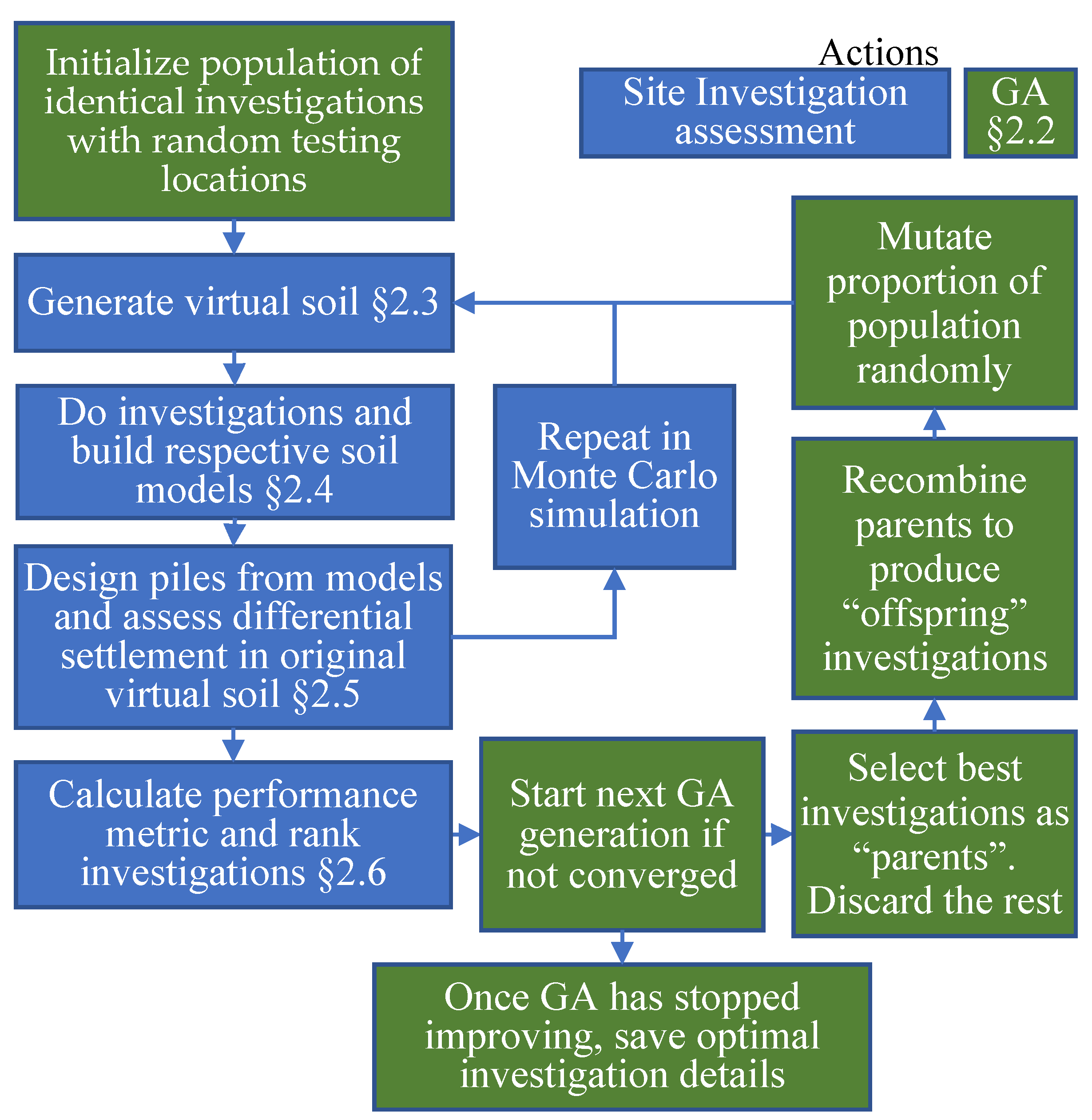
An overview of the procedures is given in the following sections. Where additional background or verification is needed, the authors refer the reader to [8] for general information, and [23] for information specific to the genetic algorithm or software involved. The latter document also acts as a succinct version of the essential information from the former. A flow chart showing the location optimization process is shown in Figure 1, which summarizes steps associated with the GA and the core investigation assessment components.

2.2. Genetic Algorithm

The analysis involves the use of a GA modified from [5]. When optimizing the locations of n boreholes, a large population of members is generated. Each member is identical, consisting of n boreholes, albeit with different, randomly assigned locations. The population then iteratively evolves, where each iteration is termed a ‘generation’. At each generation, the members are ranked from fittest to least fit, and the worst 50% are discarded. They are then replaced by ‘children’ of the fittest 50% of the population by randomly combining x and y coordinates of borehole locations through a uniform, single-point crossover method. The parents of the children are paired through ‘roulette wheel’ selection, which is a weighted random process, such that higher performing investigations are more likely to mate than less fit ones. After this stage, random members of the population, potentially including the ‘parents’ (the fittest 50%), are mutated. Mutation consists of randomly replacing x and y borehole coordinates with new ones that are picked, across the full soil profile, according to a uniform random distribution. The two processes of crossover and mutation must be applied in balance in order to fully optimize the solution. This is because the former moves the population towards a global optimum, while the latter serves to explore the solution space and help escape local optima. Assuming this balance is reasonable, a population member will find the global optimum, given enough generations.

One of the modifications to the algorithm provided by [5] was the addition of elitism; members of the population that are immune from mutation, and so are guaranteed to pass to the next generation unchanged. A single elite member was specified to ensure that the optimal solution is saved across generations, and so performance cannot deteriorate. Furthermore, the nature of the initial population was customized to this problem. As common sense suggests that boreholes are best located in proximity to piles, as demonstrated by [24], the initial population was crafted to exploit this pattern. Specifically, the initial population was created by generating normally-distributed offsets from pile locations, when the number of boreholes is a multiple. For other numbers of boreholes, offsets were generated from points that were evenly spread over a regular grid across the foundation.

Ten-thousand Monte Carlo realizations are used in each generation, which is a conservatively high value. The analysis benefits from the extra precision owing to the comparison of identical numbers of boreholes.

2.3. Virtual Soils and Site Description

Virtual soils are a 3D volume of soil properties represented by a discrete grid of elements. Each element represents the properties of the field at its location. This study employs the use of randomly-generated virtual soils, known as random fields, that have a set of smoothly-varying properties [25]. The properties of these fields are described by three statistical parameters; that is, the mean, standard deviation, and scale of fluctuation (SOF). The standard deviation, more usefully normalized by the mean to produce the coefficient of variation (COV) parameter, describes the magnitude of variation across the soil. The SOF on the other hand describes the spatial relationship of properties, as it is the distance over which properties are correlated (autocorrelation), similar to the range parameter in geostatistics.

The random fields are generated with the local average subdivision (LAS) method [26], which is known for being relatively fast and accurate [27], and is commonly used in this area of research [11]. The autocorrelation is described by an exponential Markov model. As random field generation is a minor component of this framework; it is not elaborated on here owing to space constraints, and the authors direct the reader to the references given above for further information.

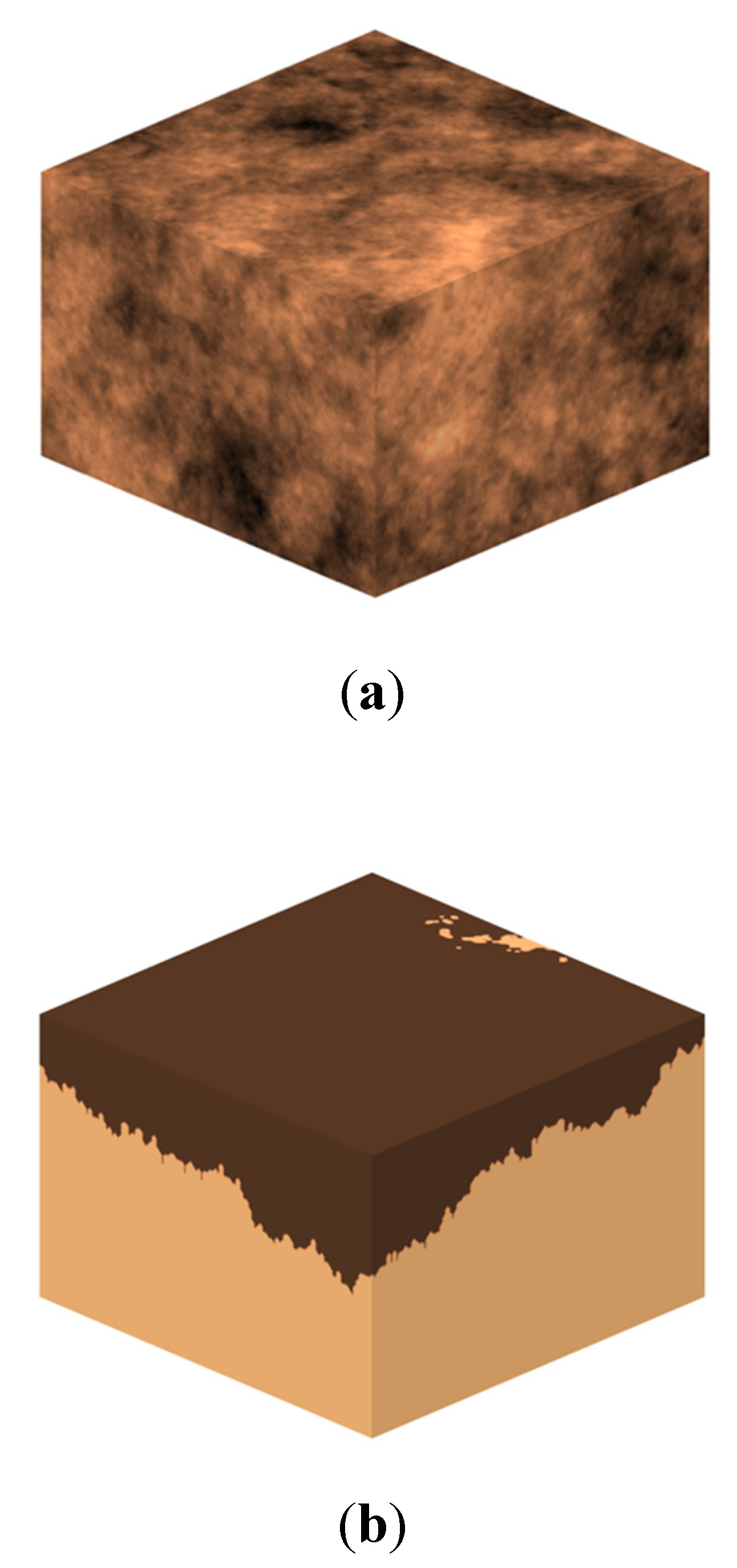
The soil properties in the single-layer case are represented by 3D random fields. These fields are generated according to a lognormal distribution [6], which ensures that properties are non-negative, and there is evidence that this distribution is appropriate for soils [28,29]. Only Young’s modulus is generated as a random field, while Poisson’s ratio is a constant at 0.3, as the impact of varying this parameter is negligible [30,31]. Examples of virtual soils used in this study are given in Figure 2, with a single-layer profile in Figure 2a. As layer boundaries are not present in this scenario, the suggested borehole locations are optimal exclusively for the purpose of determining soil properties within layers.

The single-layer soils in the present study consist of 0.5 m cubic elements, making up an 80 × 80 × 40 m volume in the horizontal (x, y) and vertical, (z) dimensions, respectively. However, instead of generating each soil individually, as is done typically, a single, large 960 × 960 × 640 element soil is produced, and each site is taken as a random subset of this large volume. While this results in considerable overlap of soil profiles across the Monte Carlo realizations, this has a negligible impact on the average field statistics, as even a small offset in three dimensions can produce an effectively different soil in regards to the foundation response.

There are two benefits to this soil subset method. Firstly, the random field is only generated once, instead of being regenerated in each GA generation. Secondly, a single larger field is generated far more quickly than numerous small fields, as there is a much smaller total volume being generated. Between these two factors, computation time is notably reduced by approximately 40 min per generation. The analysis of small numbers of borehole can then be done in under one minute.

Multi-layered soils are treated separately from the single-layer case. Rather than having material properties that smoothly vary with distance, the properties within each layer are uniform and constant. However, each layer is separated by a boundary that undulates randomly with depth, as seen in Figure 2b. As a result of this treatment, any soil uncertainty is explicitly owing to the layer boundary. The boundaries themselves are represented by 2D random fields, where elements of the 2D field represent the layer’s depth at its location. Similar to the single-layer soils, the 2D fields are generated using LAS, where the depths are normally distributed as opposed to lognormal. Further information about random fields for building multi-layered virtual soils is detailed by [24].

Owing to the wide variety of foundations and soil types examined in this study, it is impossible to specify a single mean Young’s modulus (E) for each layer while having similar pile lengths. Therefore, to facilitate relatively straightforward comparison of the results, each layer’s E value is customized to achieve a consistent average pile length. In the single-layer scenario, the target average length is 5 m, as this maximizes the number of Monte Carlo realizations where valid pile designs are achieved. Invalid designs occur when the required pile length is larger than the allowable maximum of 20 m for single layer soils and 40 m for multi-layered soils. For the multi-layer scenario, the target average pile length is 15 m to ensure that the base is embedded within the lower layer. In both scenarios, the custom E values are found by iteratively decreasing the overall soil stiffness, which in turn increases the pile length, until the target length is achieved.

It should be noted that the average pile length is not considered to have a notable impact on the optimal borehole locations in the horizontal plane. Furthermore, the specific value of mean Young’s modulus is not a source of uncertainty, as opposed to its COV. Therefore, as the mean value is consistent among both the site investigation results and the soil used for true pile settlement, it has no effect on site investigation performance. For these reasons, the mean value of Young’s modulus is largely irrelevant in the context of this research, such that the scaling of this value for an appropriate pile length, maximizing the number of valid Monte Carlo realizations, is a more important consideration.

2.4. Site Investigation

The site investigations are conducted by extracting columns of elements from the virtual soil at nominated drilling locations. As previously discussed, the test type and testing errors do not impact optimal locations. As such, the sampling is treated as being perfectly accurate, where the properties at sampled locations are known exactly. The sampling is continuous with depth, not unlike a cone penetration test (CPT); however, the sampling increment is 0.5 m as dictated by the element size. The borehole depth was found to have negligible impact on optimal testing locations in variable, single-layer soils by [1]. The authors expect this conclusion to extend to multiple-layer soils if the boreholes are guaranteed to encounter all relevant layers.

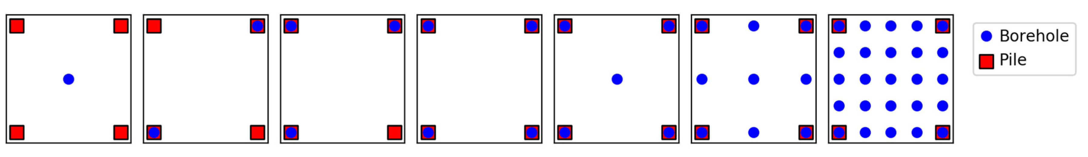
The performance of optimal testing locations obtained from this study are compared to equivalent investigations with boreholes arranged in a regular grid, as seen in Figure 3.

2.4.1. Single-Layer Case

Once samples are collected in the single-layer case, it is necessary to reduce the set of stiffnesses to a single representative value (E_red). Such a transformation is henceforth referred to as a reduction method. The so-called ‘standard deviation’ (SD) reduction method is used in the present study, which involves taking one geometric standard deviation below the geometric mean of stiffness values. In other words, E_red = μ_ln/σ_ln, where μ_ln and σ_ln are the mean and standard deviation of the natural logarithm of sample values. Sampling is taken to a depth of 20 m, the maximum allowable length of pile.

The SD method was recommended by [1] with regards to optimizing a single borehole’s location, as it was found to produce a smoother fitness landscape than less conservative recommendations. Furthermore, the resulting performance was less sensitive to borehole location, which is desirable in practice. The standard deviation method was used by [2,14,19,20,22], with [19] concluding that it provided the lowest expected total project cost when compared with a variety of reduction methods.

It is important to note that the soil model, being a uniform value, is a simplified interpretation of investigation data, compared with the full variation of the true soil. This simplification has two implications. Firstly, if all elements of the soil were tested such that the site is fully known, the foundation will still experience differential settlement owing to local discrepancies between the site and model. Secondly, and perhaps more importantly, there is no explicit relationship between the sample locations and foundation performance; it is the collection of sample values that is relevant, as opposed to their order. In other words, the sample location is not considered in the soil model. As such, the relationship between testing locations and foundation performance is implicit and is derived from the autocorrelation between the sampled soil and the soil at each pile location. On average, samples within the autocorrelation distance from the pile should be similar. However, the sample values may still be different in a given Monte Carlo realization because of the random nature of the soil, illustrating the importance of the Monte Carlo framework.

2.4.2. Multiple-Layer Case

A number of idealizations are applied to the site investigation process for the purpose of computational efficiency, owing to multi-layer soils having uniform properties in each layer. Firstly, the soil properties within each layer are known exactly, regardless of the number of samples. Secondly, the layer boundaries at borehole locations are known exactly. Any errors in depth estimation due to subjectivity or ambiguity from soil mixing at the interface are not considered.

Despite the discrete 0.5 m element size, the layer boundaries are continuous in that depths are not rounded to 0.5 m increments. Sampling is taken continuously to a total depth of 40 m, which is consistent with the bottom of the soil profile. As such, it is impossible for layer boundaries to pass underneath the bottom of the sampling.

Once the virtual investigation is conducted, a soil model is created based on the known depths of layer boundaries at borehole locations. In this model, the boundaries are interpolated from boreholes through Delaunay triangulation [32]. Extrapolation is achieved with a convex-hull expansion that approximates the layer extending outwards horizontally from the outer-most points [23].

Unlike the single-layer case, there is an explicit relationship between the soil model and the true soil. If the full surface was sampled, then the layer boundaries, and thus the full soil, would be known exactly. However, unlike that study, only local information is used; that is, the three nearest boreholes that form a triangle around the pile of interest. This is elaborated on in the next section.

2.5. Pile Settlement

Two models are needed for determining pile settlement, for single-layer and multi-layer soils, respectively. Between the 10,000 Monte Carlo realizations, and the iterative nature of the GA, billions of piles must be designed and assessed, necessitating an efficient settlement model and calculation procedure that is tailored to each soil case.

The building’s weight is equally distributed among the piles. A combined dead and live loading of 8 kPa is applied to each floor of the structure. Therefore, for the 10-story, 40 × 40 m building examined in this study, there is a total weight of 128,000 kN. All piles are designed to a differential settlement tolerance of 0.0025 [33,34].

2.5.1. Single-Layer Case

One important optimization for single-layer soils is that the true settlement of each pile, used in the differential settlement calculations, is pre-processed prior to use of the GA. This processing produces a continuous function of settlement in terms of pile length. Owing to the assumed linear-elastic mechanics, these functions can be scaled linearly with applied load and soil stiffness. As such, as applied load, soil stiffness and designed pile length are known, so too is the true settlement.

These settlement functions are generated for a given pile in a given Monte Carlo realization by determining the settlement at discrete 1 m intervals in the variable, virtual soil. These data are then made continuous through Akima interpolation [35]. The settlements at the 1 m intervals themselves are evaluated through an efficient analogy to finite element analysis (FEA), which serves as the second optimization.

This FEA equivalent, called the pseudo-incremental energy (PIE) method [36], approximates FEA results within a Monte Carlo framework within a fraction of the computational time. Elimination of FEA, the main computational bottleneck, saves several months of simulation per soil case in the single-layer scenario. It works by removing the need for FEA within the Monte Carlo simulations. Instead, only a single instance of the FEA model is needed prior to commencement. For each 1 m pile increment, a deterministic settlement value (S_det) is found through FEA in a mesh with uniform properties, for an applied unit load of 1 kN. This mesh is also used to obtain a weight (W) for each soil element. Each weight is calculated from the stress (σ, τ) and strain (ε) components in the corresponding FEA mesh element, as given in the following equation:

$$W={\sigma }_x{\epsilon }_x+{\sigma }_y{\epsilon }_y+{\sigma }_z{\epsilon }_z+{\tau }_{xy}{\epsilon }_{xy}+{\tau }_{yz}{\epsilon }_{yz}+{\tau }_{xz}{\epsilon }_{xz}$$

To determine the true settlement (S) of that length of pile in a given virtual soil, the deterministic settlement (S_det) is scaled by the weighted geometric average of soil surrounding that pile (E_eff). S = S_det/E_eff. The soil weights reflect the premise that soil properties closer to the pile have a greater influence on its settlement. Therefore, as the soil’s distribution of stresses and strains vary with the length of the pile, the weights and thus E_eff must be determined for each pile length individually.

The final optimization involves the design of piles from the soil model. The process is almost identical to that of finding the true pile settlement discussed above. However, instead of scaling each increment of the settlement curve by E_eff, the whole curve is scaled by the reduced E_red from the site investigation. Therefore, as the applied load, soil model stiffness, and settlement design tolerance are known for a given investigation, so too is the pile design.

2.5.2. Multiple-Layer Case

All pile settlement analysis, in the multiple layer scenario, is undertaken using a load transfer technique modified from [37]. The shaft stiffness is represented as a series of distributed springs (Winkler assumption). The base resistance is calculated separately, and originally by using the stiffness of the layer on which the pile is based. The modification here consists of calculating the base stiffness as a weighted harmonic average of soil stiffness below the pile base. The weights are determined by integrating an exponential decay of importance with depth below the pile, and the half-life of this decay is 3 m. The advantage here is that pile behavior can account for deeper soil layers, which more accurately matches the results from FEA [23]. Each pile’s settlement is calculated individually, using local layer boundary depths. The elimination of FEA from this scenario reduces the length of the simulation from several years to several hours.

Once the soil model is generated, as described in the previous section, it is used for pile design. This design process is undertaken by iteratively increasing the pile length until the settlement criteria is satisfied. True pile settlement is then found by taking the final design and applying the settlement model using the original, full, variable layer boundaries as generated by the 2D random fields.

It should be noted that the settlement model is designed for 1D soil profiles, where the soil properties within each layer are uniform. While the latter constraint is valid here, the former assumes that the layer boundaries are flat and horizontal, which is not the case. However, the authors of [2] found that undulating 2D layer boundaries can be represented by a single, effective depth by taking an inverse-distance-squared weighted average of layer depths around the pile, thereby reducing the soil to a 1D equivalent. This technique is used for calculating true pile settlement.

However, to reduce computational time, the layer depths are taken directly from the interpolated surface at the pile’s location. In other words, a single depth value is used as opposed to a local average. This approximation is reasonable for the soil model, as opposed to the random fields, as there is far less local variation due to the linear interpolation of scattered data. Furthermore, as the interpolated surface consists of triangular planes with vertices defined by borehole locations, a point inside each triangle is also a weighted average of the layer’s depth at each borehole. A comparison has found that this optimization has a negligible impact on the optimal locations in this study, while further reducing computational time by an order of magnitude. This reduction, from roughly an hour to several minutes, is owing to the significantly reduced amount of 2D interpolation required for a series of discrete points versus an entire plane.

2.6. Differential Settlement and Failure Cost

Once the true settlement for each pile is obtained in a Monte Carlo realization for an investigation, the differential settlement can be determined. This involves finding the difference in settlement between all combinations of two piles in the foundation as a proportion of the distance between the piles. The final differential settlement for that foundation is taken as the maximum value of all combinations.

While the geometric product metric is used by the GA for optimization, the failure costs associated with the recommendations are also calculated. A comparison of these costs gives a more meaningful representation of the benefit of using optimal testing locations over a regular grid.

Previously, a relationship has been derived for failure cost in terms of differential settlement by [8]. The relationship is based on levels of structural cracking associated with magnitudes of differential settlement by [38], and the cost of repairing that cracking [39]. In essence, an insufficient investigation is likely to result in higher differential settlement on average, requiring a greater repair cost.

This relationship itself is represented by a linear function, such that a differential settlement value of 0.003 results in A$0 of failure, and 0.009 results in a failure cost equal to the building’s construction cost (C_c). The construction cost, in this case, A$47,600,000 [39], is analogous to demolishing and rebuilding the structure as a result of excessive cracking. As such, this linear function is bounded by a minimum of $0 and a maximum of C_c. The costs are calculated individually for each Monte Carlo realization, which are subsequently averaged to form the expected failure cost.

3. Results and Discussion

Prior to analyzing the results in the following sections, it should be noted that, while properly configured GAs perform well at finding solutions that are near a global optimum, they are quite inefficient at finding the exact solution. Therefore, rather than taking the results as absolute recommendations, a degree of subjective interpretation is required. One example of subjective interpretation is the consideration of symmetry. If the pile configuration is symmetrical in one or more axes, and if the number of boreholes allows for a symmetrical solution, the true optimal locations should be re-interpreted as such.

3.1. Analysis of GA Parameters

The choice of optimal GA parameters is known to be problem-specific [5]. Therefore, when a GA is introduced to a new problem, as in the present situation, it is necessary to analyze the parameters that produce the best results in terms of quality and processing time.

This analysis is undertaken here with a single-layer soil of COV 80% and SOF of 10 m. The single-layer scenario is considered, as the overall analysis is faster and more efficient than that of the multi-layer scenario, allowing for a wider range of parameters to be assessed. It should be noted that the solution space is slightly different between the two soil scenarios owing to the manner in which the soil models are constructed, as described previously. However, the nature of the problem is similar, and so the results are expected to be transferable.

Two GA parameters are investigated with regards to the solution evolution; that is, the population size and mutation rate. Between them, the values are 250 and 500, as well as 1, 2, 5, and 10%, respectively, resulting in eight combinations being assessed.

Furthermore, it is important to specify a stopping criterion so that the algorithm concludes after an appropriate number of generations, beyond which there is little improvement. The criterion is needed because it is impossible to know in advance when the GA has found an optimal solution. As such, it must instead detect if the solution has remained relatively unchanged for a specified number of generations, implying convergence. The two additional parameters are the performance tolerance, such that improvement below this threshold is considered negligible, and the number of consecutive generations, which must have negligible improvement.

For each case, a tolerance of 0% is used along with 20 generations of consecutive values, meaning that the solution must be unchanged over this time. Furthermore, once the GA has converged, it is restarted with a new population created from randomly generated offsets from the optimal solution, in an attempt to find a nearby optimum. This second stage is set to have 0% improvement for 10 consecutive generations before stopping. The use of such a conservative, strict stopping criterion allows for the evolution curves to be analyzed for alternative, less strict criteria, without having to re-run the GA.

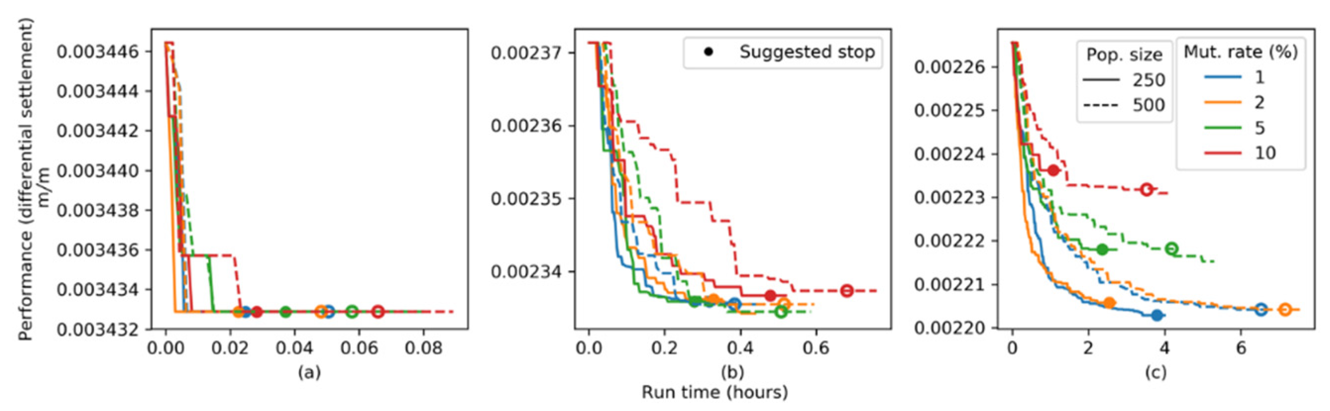
Plots showing the evolution of performance are given in Figure 4 for the cases of 1, 5, and 25 boreholes with a nine-pile, 40 × 40 m building, comparing the aforementioned mutation rates and population sizes. Other building cases not shown here include buildings of 10 × 10 m, 20 × 20 m, and 30 × 30 m with a variety of numbers of piles and pile spacings. It should be noted that there are no clear trends across the different building cases, and the plots in Figure 4 should not necessarily be taken as expected trajectories. Nevertheless, some general conclusions can be made.

The interpretation of Figure 4 is that, as the performance value decreases over successive iterations, the boreholes physically move to more optimal locations. Although counter-intuitive, lower performance values are more desirable, as there is a reduced likelihood of excessive differential settlement. The changes between iterations can vary greatly, from one borehole moving a small distance owing to the best solution being improved, to all boreholes being moved extensively when an entirely new optimal solution is found. This latter case results in the sudden large drops in performance value, while the former is typically responsible for the segments of gradual, smooth improvement.

For small numbers of boreholes, in the order of 1–2, the solution converges quickly, regardless of parameter choices. For intermediate numbers, from 3–8, the progression is stepped (staggered) with several generations in a row stalling with no improvement. For 9 and more boreholes, improvement tends to be relatively smooth and continuous.

Upon inspection of various sets of building sizes and numbers of piles, not shown here owing to space constraints, the authors conclude that a population size of 500 and a mutation rate of 1% is the single best choice towards finding the optimal locations in all cases. Higher mutation rates, particularly above 2%, introduce a sufficiently high degree of randomness to prevent solution convergence, most easily seen in Figure 4c.

Regarding the stopping criteria, the number of consecutive generations parameter was found to be more important than the performance tolerance, owing to the stepped improvement, most readily seen in Figure 4b. Examining a range of generation numbers and tolerances across the building cases revealed that the recommended stopping parameters are 20 consecutive generations and a tolerance of 2.5 × 10⁻⁵, or 0.0025%.

The run time needed for convergence increases exponentially with the number of boreholes. This is logical, as the solution space increases exponentially, and the time needed for individual generations also increases with the number of boreholes.

3.2. Single-Layer Analysis

A wide variety of analyses have been undertaken with respect to finding optimal borehole locations in variable, single-layer soil. While not shown here, the analysis includes examining the effect of COV, test type, and reduction method, as done in the case of a single borehole by [1]. It was found that optimal testing location was not noticeably affected by these parameters. This insensitivity is intuitive as the site and sampled data do not structurally change in these cases, other than a uniform shift in variability with COV. This conclusion for multiple boreholes is consistent with the analysis by [1]. These results indicate that the optimal borehole locations discussed here can be fairly generalized across different soil cases. However, there is some variation in the results with SOF, which is discussed later. Similarly, optimal borehole locations were found not to change, relative to the piles, for different foundation areas. In other words, the optimal borehole pattern scales proportionately with the building area. The authors expect this scaling to apply to different aspect ratios of building footprints, although further work is needed on this variable.

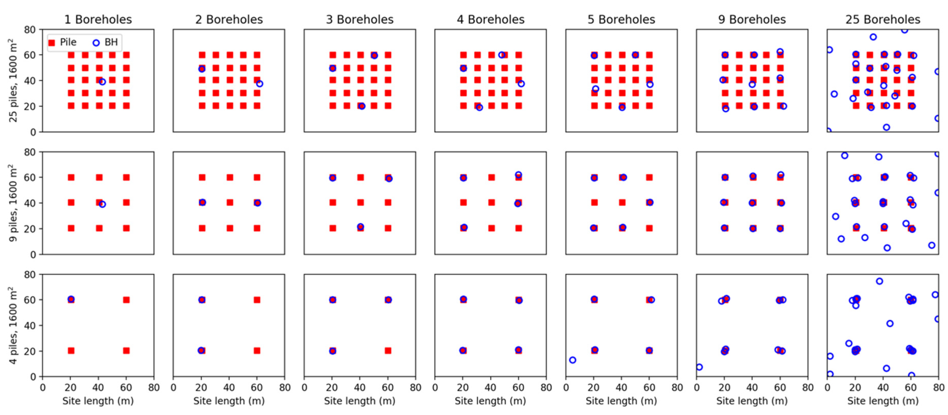
A set of optimal testing locations has been shown for a 40 × 40 m building with varying numbers of piles in Figure 5, for a soil of COV 80% and SOF of 20 m. Several clear trends can be observed. For example, when the number of boreholes is less than or equal to the number of piles, the boreholes should be placed at the piles. A single borehole should be placed at the center-most pile in the building. In the case of two boreholes, they should be placed at the sides of the building rather than the corners, as this means the distance between them and the furthest piles is minimized. For the same reason, three boreholes should be placed so as to form an equilateral triangle as much as possible, while still being in close proximity to piles.

For other borehole cases, the results become more difficult to interpret owing to an apparent randomness in the data. It has previously been noted that borehole locations given by the GA may not be truly optimal, as it is possible that the GA has not fully converged on a global optimum. In the case of single-layer soils, there is an additional source of randomness discussed by [1] in the form of random bias in the soil when averaged across Monte Carlo realizations. This bias is in the order of roughly 2.5% of the soil COV, which, in most analyses, would be considered negligible. However, it is possible that, when optimizing borehole locations, the GA may have a subtle preference to place boreholes at locations where the averaged stiffness is underestimated. This bias is most likely owing to a low-level correlation or other unavoidable imperfections in the random number generator. Either the lack of convergence or the random bias could be responsible for the observed random scatter.

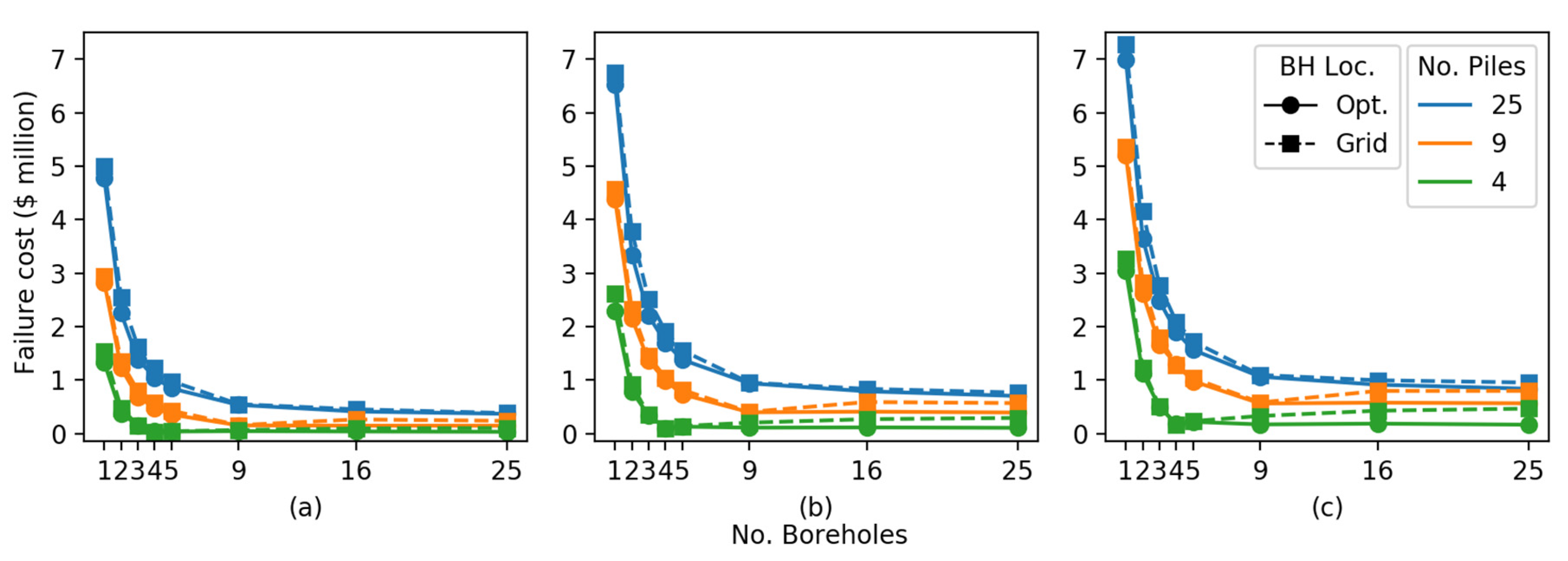
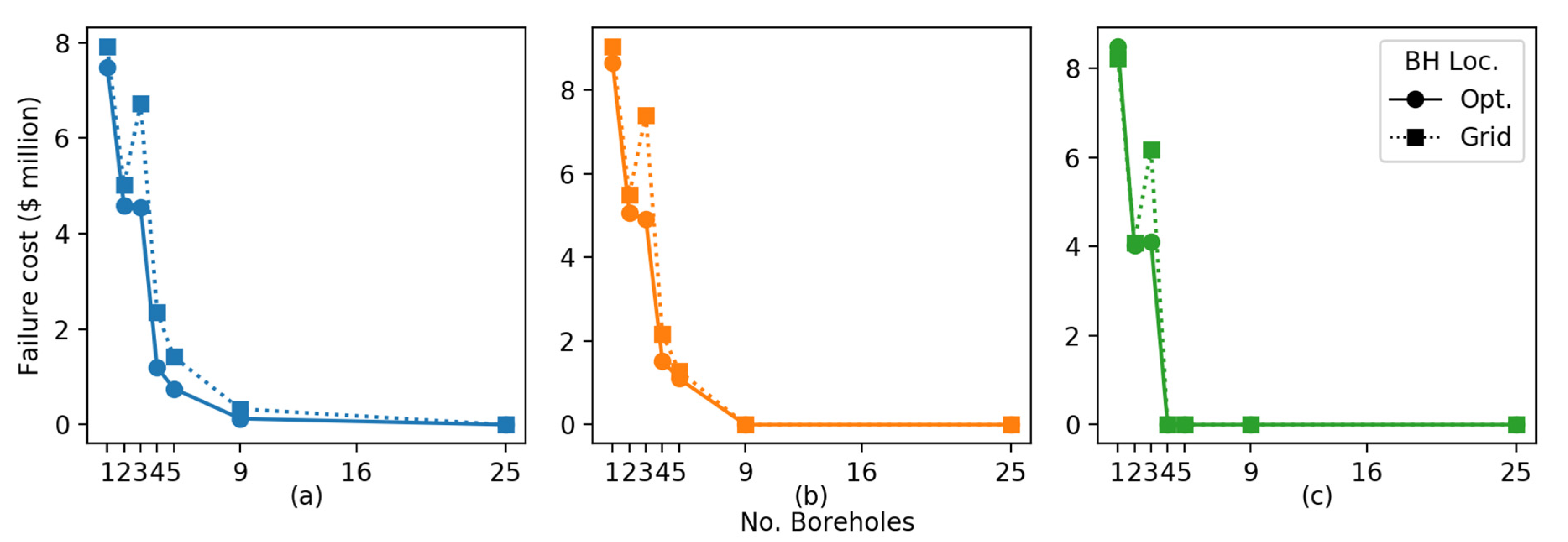
It is worth noting that the optimal locations shown in Figure 5 may have only a minimal advantage over a regular grid layout, such as those seen in Figure 3. For this reason, 6 is included, which compares expected failure costs between the suggested locations and regular grid locations for a variety of boreholes. The costs are given for all three building and borehole cases, for soils with an SOF of 10 m, 15 m, and 20 m. Analysis of this figure will be included along with that of Figure 5 for the remainder of this section.

Furthermore, there is excessive randomness for high numbers of boreholes and a large SOF relative to the pile spacing, most easily seen in the 25 borehole, 25 pile case where a regular grid is expected. In these specific high borehole cases, the apparent randomness is owing to the GA intentionally spreading boreholes across the full site. A large spread increases the likelihood that at least some low stiffness samples are collected on average, leading to a more conservative soil model. This manner of added conservativism is the only type allowed by the model, as opposed to more traditional mechanisms such as loading safety factors. Therefore, this random spread of boreholes is an artefact of the artificial nature of the problem, and such random locations should be ignored. Instead, a regular grid is recommended. Indeed, upon examination of the costs in Figure 6, there appears to be little benefit to using the apparent random scatter of 25 boreholes over the regular grid in the case of 25 piles. A similar effect is noted when the SOF is large relative to the building footprint, whereby some boreholes are randomly scattered away from the pile locations even for small numbers of piles and boreholes. These results are not shown visually owing to space constraints, and it is worth reiterating that the improvement over regular sampling is negligible.

With this disregard for the random borehole locations in mind, reinterpreting the results for the expected symmetry, additional trends can be identified. When there are more boreholes than piles, the former should be distributed evenly across the locations of the latter. This is most evident in Figure 5 with four piles and nine boreholes, where there are two of the latter at each pile, as well as with 25 boreholes, where there are four at each pile. Upon examination of the failure costs in Figure 6c for a nine- or four-pile building, there can be a reduction in expected cost in the order of A$300,000 by adopting this recommendation in soils with a high SOF. However, this is largely a moot point as the same failure cost can be achieved with fewer boreholes.

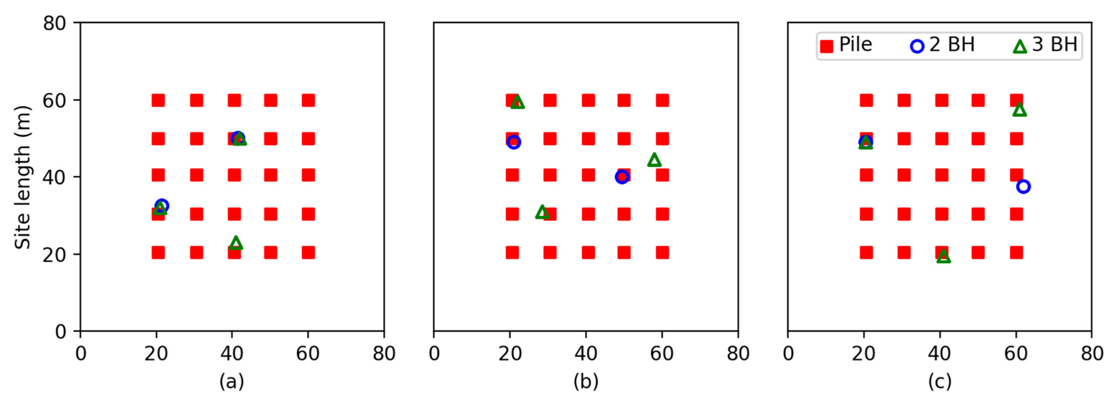
As mentioned earlier, there is a variation in optimal testing locations as the SOF changes. This is most apparent in the case of two or three boreholes and 25 piles. The large number of piles facilitates flexibility in borehole locations as they should be drilled at a pile, allowing the effects of SOF to be highlighted. The above case is shown for an SOF of 10 m, 15 m, and 25 m in Figure 7. It can be seen that, as the SOF increases, so does the recommended borehole spacing. While this spacing appears to be approximately double that of the SOF, it is difficult to define an explicit relationship owing to the possibility of the randomness discussed previously. Therefore, optimal borehole spacing with regards to SOF is an area for future research. The relationship does not apply for small or large SOFs. In the former case, a wide variety of sample values is encountered by each borehole, which, when locally averaged, results in a similar performance for all testing locations. For large SOFs relative to the building footprint, the soil becomes relatively homogenous and constant, and so again, performance varies little with testing location. The optimal locations for other numbers of boreholes do not notably vary with SOF, particularly when ignoring apparent randomness.

In conclusion, the main, overriding suggested rule is to place boreholes in close proximity to piles. Additional suggestions vary depending on the number of boreholes. Two should be placed so as to minimize the distances between either of them and the furthest pile. Three should be placed so as to form an equilateral triangle within the building footprint. If possible, borehole spacing can be double that of the horizontal SOF for small numbers of boreholes. However, this is considered as being of secondary importance, particularly as it is impossible to determine the SOF of a site without already having done extensive soil testing. If there are more piles than boreholes, then a regular grid over the building footprint, at pile locations, is recommended.

3.3. Multiple-Layer Analysis

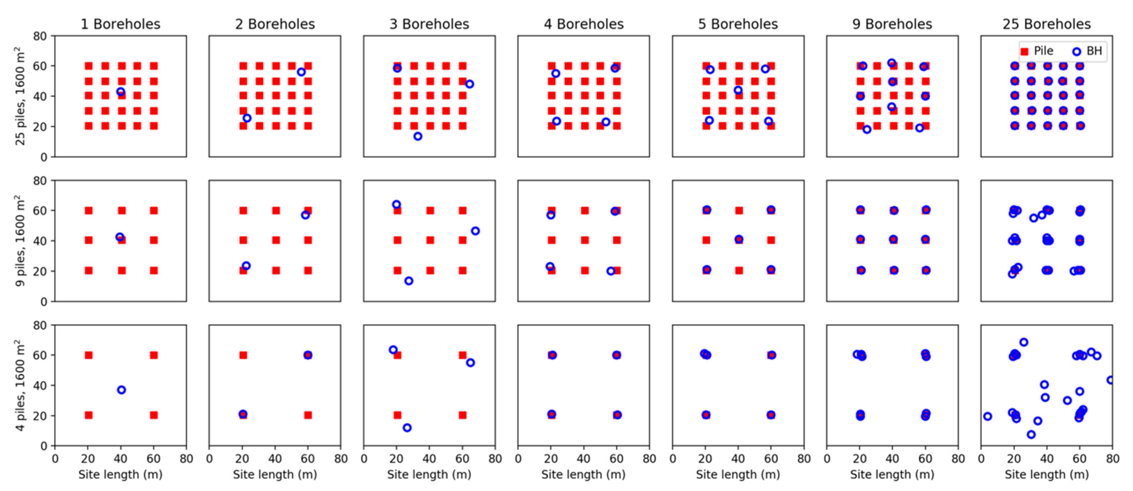
This section discusses recommended testing locations for the purpose of delineating layer boundaries, without consideration for determining material properties. The optimal locations for a two-layer soil case are shown in Figure 8, for a layer stiffness ratio of 1:9, an average boundary depth of 10 m, a boundary SOF of 100 m, and a boundary undulation standard deviation of 2 m. This soil is similar in appearance to that shown in Figure 2b, albeit with a reduced magnitude of vertical boundary variation. Further information on these parameters is given by [24].

The stiffness ratio and degree of undulation were found to have a negligible impact on the recommended borehole locations, when alternate values of these parameters were assessed. Logically, while these parameters would alter the overall magnitude of differential settlement, they would not impact the relative differential settlement between different testing locations. Furthermore, the authors of [22] have shown that the exact SOF of the layer boundaries has a negligible impact on the performance of pile foundations when the value is more than twice as large as the building footprint, as is the case here. Owing to the relative insensitivity of the results to the aforementioned parameters, it is expected that the following recommendations can be generalized to a wide variety of multi-layer soils. As with the single-layer case, the optimal borehole patterns were found to scale with the building area.

Upon inspection of Figure 8, the locations are more intuitive and less random compared with the single-layer case. The apparent randomness from before is not present, except for the cases of 25 boreholes with four or nine piles. Here, it should be noted that three boreholes in close proximity to a pile give complete knowledge for that pile, meaning that the additional boreholes are not considered in the pile’s performance. As such, as with the single-layer soil, boreholes should generally be positioned evenly near pile locations.

A single borehole should be placed at the center of the building in all cases, as is expected. This recommendation could also be argued to extend to the single-layer scenario, as [1] showed that a central location is ideal in terms of failure cost for four piles and a large horizontal soil SOF. This is in contrast to the geometric product metric used in the optimization process, which is generally in good agreement with the failure cost in all other building and SOF cases.

Two boreholes should be placed at the corner of the buildings in the four-pile case. As the pile density increases, these two boreholes are best placed closer to the building center so as to better represent the central piles. The authors suggest that the two boreholes should never be placed more than one pile row in from the outer edge, in order to minimize extrapolation of the layer to outer piles. In other words, if the pile spacing is 5 m, the boreholes should never be more than 5 m away from the building’s perimeter. When three boreholes are used, they should be placed so as to form an equilateral triangle over the building while being in reasonable proximity to a pile, in a manner similar to the single-layer scenario. The difference here is that the triangle is notably larger, so as to minimize extrapolation to outer piles. For this reason, testing in close proximity to a pile is less critical compared with forming an equilateral triangle that covers the majority of the building.

When using four boreholes, testing at or near the corners is optimal, moving the boreholes slightly inward with increased pile density as in the two-borehole case. This can be said for five boreholes as well, with the fifth borehole being centrally located or at one of the corners, if there is no central pile. In all other cases, a regular grid of boreholes across the building footprint is recommended, as is the case of 9 or 25 boreholes with the 25-pile building. While the 9 boreholes over 25 piles have a fairly triangular pattern, the authors suspect that this is an artefact of the layer interpolation method, which uses triangulation. As such, a regular grid with a rectangular pattern is recommended.

As done above with Figure 6, the failure costs for each pile and borehole case, for the aforementioned two-layer soil, are presented in Figure 9. A consistent observation in Figure 9 is that there is significant improvement in the three-borehole case using a rotated equilateral triangle instead of placing each borehole at the three piles directly. This saving is in excess of A$2 million, or 4.2% of the building’s construction cost. Interestingly, three boreholes placed in the regular grid pattern have considerably worse performance than two boreholes, despite the additional soil information. This degradation is owing to the layer boundary being extrapolated outside of the triangle formed by the three boreholes. As such, the fourth pile, without an associated borehole, is likely to be misrepresented in the soil model. It must be remembered that the addition of a third borehole significantly reduces the failure cost compared with two in the single-layer scenario.

For all other cases, the improvement from optimal sampling over the regular grid increases with the number of piles. Other than with three boreholes, there is a negligible difference between the optimal and grid placement in the case of four piles. There is moderate improvement in the nine-pile case for less than five boreholes. Similarly, there is greater improvement for 25 piles and less than 9 boreholes, in the order of A$500,000.

Further analysis was conducted on multi-layer soil profiles, including those featuring the possible formation of soil lenses. A lens is a soil layer that is laterally discontinuous, such that it can be present at one borehole or pile location and absent from another. Understandably, this circumstance is particularly detrimental to foundation performance. However, optimal testing locations do not notably change from that seen in Figure 8. As such, those locations are also recommended in soils with three or more layers.

Comparing the improvement between the single-layer and multi-layer scenarios, the cost savings are noticeably higher in the latter case. This improvement is owing to the more explicit relationship between borehole locations and the soil model for the layer boundaries. Therefore, as the foundation performance is less sensitive to the exact borehole locations in the single-layer case, the authors suggest using the multi-layer recommendations in practice. This suggestion is reinforced by the overall similarity of recommendations between the two soil scenarios, and that the multi-layer recommendations are less random.

4. Conclusions

This study has demonstrated that a genetic algorithm (GA) can be used to optimize borehole locations with respect to improving foundation performance. An analysis of GA parameters reveals that the best overall configuration is a low mutation rate in the order of 1–2% and a large population such as 500 members. The recommended stopping criterion, used to assess when the GA has converged on a global solution, is when there has been less than a 0.0025% improvement on the previous generation for 20 consecutive generations.

Optimal borehole locations have been derived independently for single-layer soil and multi-layer soils. These scenarios examine what is optimal for determining the material properties of layers and layer boundaries, respectively. The recommended testing locations were generally similar across the two scenarios. However, locations appeared somewhat random in the single-layer soil owing to an implicit relationship between the sample locations and soil model. As this relationship is explicit in the multi-layer case, and because the cost savings were greater, the optimal multi-layer locations are recommended for general use. The difference in failure cost between the optimal and regular grid patterns varied greatly, from being negligible through to over A$2 million, or 4.2% of the building’s construction cost in the case of three boreholes.

A large number of variables were identified as having no or negligible effect on optimal borehole locations. In the single-layer scenario, this includes the coefficient of variation, test type, and reduction method. The optimal borehole spacing appeared to increase with the scale of fluctuation (SOF) in the case of two or three boreholes. However, the relationship between borehole spacing and SOF requires further analysis, ideally with anisotropic soils where the vertical SOF is held constant. A high SOF relative to either the borehole spacing or building footprint results in increasingly random borehole locations being preferred. However, the improvement due to this random sampling is negligible, such that the final stated guidelines are recommended. In the multi-layer scenario, the degree of layer undulation, layer stiffness ratio, and number of layers appear to have little effect on the results. Similarly, the building area has little impact on the optimal borehole pattern, as locations scale linearly with footprint size.

The recommended testing locations for all soil conditions are as follows:

• The general rule is that boreholes should be placed in close proximity to piles, unless stated otherwise;
• A single borehole should be located in the center of the building;
• Two boreholes should be placed at the building corners;
• Three boreholes should be arranged as an equilateral triangle, rotated to be in proximity to piles and containing the majority of the building within its area;
• With four or five boreholes, the outer-most ones should be moved closer to the center as pile density increases, however, they should not be further inward than one row of piles.

Some recommendations for future research are given within this section.

Further suggestions include the use of a more advanced GA or evolutionary algorithm. For example, exploring the use of alternate selection, crossover and mutation mechanisms that are more sophisticated than the simple implementations used in the present study, such as normally-distributed mutation. The GA could also be adapted to optimize additional site investigation parameters, such as borehole depth and test type, within the same investigation. It should be noted that the results are only applicable to the design of pile foundations. Future research could analyze alternate foundations types, as well as investigations for retaining structures and tension piles for building basements, and dewatering plans. The software and source code used in this study are open source and available for use by researchers and practicing engineers.

References

- Crisp, M.P.; Jaksa, M.B.; Kuo, Y.L. Effect of borehole location on pile performance. Georisk: Assessment and Management of Risk for Engineered Systems and Geohazards. Georisk 2020. [Google Scholar] [CrossRef]
- Crisp, M.P.; Jaksa, M.B.; Kuo, Y.L.; Fenton, G.A.; Griffiths, D.V. Characterising Site Investigation Performance in a Two Layer Soil Profile. Can. J. Civ. Eng. 2020. [Google Scholar] [CrossRef]
- British Standards. Code of Practice for Site Investigations; British Standards: London, UK, 1999. [Google Scholar]
- Shukla, S.K.; Sivakugan, N. Site investigation and in situ tests. In Geotechnical Engineering Handbook; Das, B., Ed.; J. Ross Publishing: Richmond, VA, USA, 2011. [Google Scholar]
- Haupt, R.L.; Haupt, S.E. Practical Genetic Algorithms, 2nd ed.; John Wiley: Hoboken, NJ, USA, 2004. [Google Scholar]
- Ang, A.H.-S. Probability Concepts in Engineering: Emphasis on Applications in Civil & Environmental Engineering, 2nd ed.; John Wiley & Sons: Hoboken, NJ, USA, 2007. [Google Scholar]
- Jaksa, M.B.; Kaggwa, W.S.; Fenton, G.A.; Poulos, H.G. A framework for quantifying the reliability of geotechnical investigations. In Proceedings of the 9th International Conference on the Application of Statistics and Probability in Civil Engineering, Francisco, CA, USA, 6–9 July 2003; pp. 1285–1291. [Google Scholar]
- Crisp, M.P.; Jaksa, M.B.; Kuo, Y.L. Framework for the Optimisation of Site Investigations for Pile Designs in Complex Multi-Layered Soil. Res. Rep. Sch. Civil Environ. Min. Eng. 2019. [Google Scholar] [CrossRef]
- Griffiths, D.; Fenton, G.A. Seepage beneath water retaining structures founded on spatially random soil. Geotechnique 1993, 43, 577–587. [Google Scholar] [CrossRef] [Green Version]
- Fenton, G.A.; Griffiths, D. Statistics of block conductivity through a simple bounded stochastic medium. Water Resour. Res. 1993, 29, 1825–1830. [Google Scholar] [CrossRef] [Green Version]
- Fenton, G.A.; Griffiths, D.V. Risk Assessment in Geotechnical Engineering; Wiley: Hoboken, NJ, USA, 2008. [Google Scholar]
- Crisp, M.P. SIOPS (Site Investigation Optimisation for Piles Using Statistics). 2020. Available online: https://github.com/Michael-P-Crisp/SIOPS (accessed on 9 July 2020).
- Goldsworthy, J.S.; Jaksa, M.B.; Fenton, G.A.; Kaggwa, W.S.; Griffiths, D.V.; Poulos, H.G. Effect of sample location on the reliability based design of pad foundations. Georisk 2007, 1, 155–166. [Google Scholar] [CrossRef]
- Crisp, M.P.; Jaksa, M.B.; Kuo, Y.L. Influence of Site Investigation Borehole Pattern and Area on Pile Foundation Performance. In Proceedings of the 12th ANZ Young Geotechnical Professionals Conference, Hobart, Tasmania, 7–8 November 2018. [Google Scholar]
- Goldsworthy, J.S.; Jaksa, M.B.; Fenton, G.A.; Griffiths, D.V.; Kaggwa, W.S.; Poulos, H.G. Measuring the risk of geotechnical site investigations. In Probabilistic Applications in Geotechnical Engineering; ASCE Library: Reston, VA, USA, 2007; pp. 1–12. [Google Scholar]
- Crisp, M.P.; Jaksa, M.B.; Kuo, Y.L. The influence of Site Investigation Scope on Pile Design in Multi-layered, Variable Ground. In Geo-Risk 2017; Huang, J., Ed.; ASCE Library: Denver, CO, USA, 2017; pp. 390–399. [Google Scholar]
- Gong, W.; Tien, Y.-M.; Juang, C.H.; Martin, J.R.; Luo, Z. Optimization of site investigation program for improved statistical characterization of geotechnical property based on random field theory. Bull. Eng. Geol. Environ. 2016, 76, 1021–1035. [Google Scholar] [CrossRef]
- Huang, L.; Huang, S.; Lai, Z. On the optimization of site investigation programs using centroidal Voronoi tessellation and random field theory. Comput. Geotech. 2020, 118, 103331. [Google Scholar] [CrossRef]
- Crisp, M.P.; Jaksa, M.B.; Kuo, Y.L. Toward a generalized guideline to inform optimal site investigations for pile design. Can. Geotech. J. 2019. [Google Scholar] [CrossRef]
- Crisp, M.P.; Jaksa, M.B.; Kuo, Y.L. Towards Optimal Site Investigations for Generalized Structural Configurations. In Proceedings of the 7th International Symposium on Geotechnical Safety and Risk, Taipei, Taiwan, 11–13 December 2019. [Google Scholar]
- Crisp, M.P.; Jaksa, M.B.; Kuo, Y.L. Influence of distance-weighted averaging of site investigation samples on foundation performance. In Proceedings of the 13th Australia New Zealand Conference on Geomechanics, Perth, Australia, 1–3 April 2019. [Google Scholar]
- Crisp, M.P.; Jaksa, M.B.; Kuo, Y.L. Characterising Site Investigation Performance in Multiple-Layer Soils and Soil Lenses. Georisk 2020. [Google Scholar] [CrossRef]
- Crisp, M.P. SIOPS User Manual (Site investigation optimisation for piles using statistics). Research Gate 2020. [Google Scholar] [CrossRef]
- Crisp, M.P.; Jaksa, M.B.; Kuo, Y.L.; Fenton, G.A.; Griffiths, D.V. A method for generating virtual soil profiles with complex, multi-layer stratigraphy. Georisk 2019, 13, 154–163. [Google Scholar] [CrossRef]
- Vanmarcke, E. Random Fields: Analysis and Synthesis; MIT Press: London, UK, USA, 1983. [Google Scholar]
- Fenton, G.A.; Vanmarcke, E.H. Simulation of random fields via local average subdivision. J. Eng. Mech. 1990, 116, 1733–1749. [Google Scholar] [CrossRef] [Green Version]
- Fenton, G.A. Error evaluation of three random-field generators. J. Eng. Mech. 1994, 120, 2478–2497. [Google Scholar] [CrossRef]
- Lumb, P. The variability of natural soils. Can. Geotech. J. 1966, 3, 74–97. [Google Scholar] [CrossRef]
- Hoeksema, R.J.; Kitanidis, P.K. Analysis of the spatial structure of properties of selected aquifers. Water Resour. Res. 1985, 21, 563–572. [Google Scholar] [CrossRef]
- Fenton, G.A.; Paice, G.; Griffiths, D. Probabilistic Analysis of Foundation Settlement: Geomechanics Research Center, Colorado School of Mines. 1996. Available online: https://www.researchgate.net/publication/247256777_Probabilistic_Analysis_of_Foundation_Settlement (accessed on 9 July 2020).
- Naghibi, F.; Fenton, G.; Griffiths, D. Serviceability limit state design of deep foundations. Géotechnique 2014, 64, 787–799. [Google Scholar] [CrossRef]
- Delaunay, B. Sur la sphere vide. Izv Akad Nauk SSSR. Otdelenie Matematicheskii i Estestvennyka Nauk 1934, 7, 1–2. [Google Scholar]
- Sowers, G.F. Shallow foundations. In Foundation Engineering; Leonards, G.A., Ed.; McGraw-Hill: New York, NY, USA, 1962. [Google Scholar]
- Salgado, R. The Engineering of Foundations; McGraw-Hill: New York, NY, USA, 2008. [Google Scholar]
- Akima, H. A new method of interpolation and smooth curve fitting based on local procedures. J. ACM (JACM) 1970, 17, 589–602. [Google Scholar] [CrossRef]
- Ching, J.; Hu, Y.-G.; Phoon, K.-K. Effective Young’s modulus of a spatially variable soil mass under a footing. Struct. Saf. 2018, 73, 99–113. [Google Scholar] [CrossRef]
- Mylonakis, G.; Gazetas, G. Settlement and additional internal forces of grouped piles in layered soil. Geotechnique 1998, 48, 55–72. [Google Scholar] [CrossRef] [Green Version]
- Day, R.W. Forensic Geotechnical and Foundation Engineering; McGraw-Hill: New York, NY, USA, 1999. [Google Scholar]
- Rawlinsons, A. Australian Construction Handbook, 34th ed.; Rawlhouse Publishing Pty. Ltd.: Perth, Australia, 2016; p. 1005. [Google Scholar]
Figure 1.
Flow chart for the process of optimizing an investigation’s borehole locations. GA, genetic algorithm.
Figure 2.
Example virtual soils; (a) a single layer profile with a coefficient of variation (COV) of 80% and scale of fluctuation (SOF) of 15 m; and (b) a two-layer soil with a stiffness ratio of 1:9, boundary depth of 10 m, and boundary standard deviation of 4 m.
Figure 3.
Examples of boreholes arranged in regular grids over the building footprint, in the case of four piles.
Figure 4.
Evolution plots for a nine-pile, 40 × 40 m building and (a) 1 borehole, (b) 5 boreholes, and (c) 25 boreholes.
Figure 5.
Optimal testing locations for different numbers of piles and boreholes for a soil with a COV of 80% and an SOF of 20 m.
Figure 6.
Failure cost comparison between borehole (BH) patterns; a regular grid (Grid) and optimal locations (Opt.) for different numbers of piles, and an SOF of (a) 10 m, (b) 15 m, and (c) 20 m.
Figure 7.
Comparison of borehole spacing for a 25-pile building with a soil SOF of (a) 10 m, (b) 15 m, and (c) 25 m.
Figure 8.
Optimal testing locations for different numbers of piles and boreholes for a two-layer soil with stiffness ratio 1:9 and boundary standard deviation of 2 m.
Figure 9.
Failure cost comparison between a regular grid of boreholes (Grid) and optimal locations (Opt.) in a two layer soil with boundary standard deviation of 4 m and (a) 25 piles, (b) 9 piles, and (c) 4 piles.
© 2020 by the authors. Licensee MDPI, Basel, Switzerland. This article is an open access article distributed under the terms and conditions of the Creative Commons Attribution (CC BY) license (http://creativecommons.org/licenses/by/4.0/).
Share and Cite
MDPI and ACS Style
Crisp, M.P.; Jaksa, M.; Kuo, Y. Optimal Testing Locations in Geotechnical Site Investigations through the Application of a Genetic Algorithm. Geosciences 2020, 10, 265. https://0-doi-org.brum.beds.ac.uk/10.3390/geosciences10070265
AMA Style
Crisp MP, Jaksa M, Kuo Y. Optimal Testing Locations in Geotechnical Site Investigations through the Application of a Genetic Algorithm. Geosciences. 2020; 10(7):265. https://0-doi-org.brum.beds.ac.uk/10.3390/geosciences10070265
Chicago/Turabian StyleCrisp, Michael P., Mark Jaksa, and Yien Kuo. 2020. "Optimal Testing Locations in Geotechnical Site Investigations through the Application of a Genetic Algorithm" Geosciences 10, no. 7: 265. https://0-doi-org.brum.beds.ac.uk/10.3390/geosciences10070265
Note that from the first issue of 2016, this journal uses article numbers instead of page numbers. See further details here.